Gross domestic savings (% of GDP) - NY.GDS.TOTL.ZS

Name: Gross domestic savings (% of GDP)
Creator: François Geerolf
License: https://creativecommons.org/licenses/by/4.0/

Data - WDI

Author

François Geerolf

Last observation: 2025 (N = 161)

First observation: 1960 (N = 75)

Last data update: 04 sept. 2026, 00:27

Last compile: 04 sept. 2026, 00:40

Nobs - Javascript

Code

NY.GDS.TOTL.ZS |>
  left_join(iso2c, by = "iso2c") |>
  group_by(iso2c, Iso2c) |>
  mutate(value = round(value, 1)) |>
  summarise(Nobs = n(),
            `Year 1` = first(year),
            `Net Saving 1 (%)` = first(value),
            `Year 2` = last(year),
            `Net Saving 2 (%)` = last(value)) |>
  arrange(-Nobs) |>
  mutate(Flag = gsub(" ", "-", str_to_lower(Iso2c)),
         Flag = paste0('<img src="../../bib/flags/vsmall/', Flag, '.png" alt="Flag">')) |>
  select(Flag, everything()) %>%
  {if (is_html_output()) datatable(., filter = 'top', rownames = F, escape = F) else .}

Individual Countries

Japan

Code

NY.GDS.TOTL.ZS |>
  left_join(GC.NLD.TOTL.GD.ZS |> select(iso2c, year, GC.NLD.TOTL.GD.ZS = value), by = c("iso2c", "year")) |>
  left_join(NY.GNS.ICTR.ZS |> select(iso2c, year, NY.GNS.ICTR.ZS = value), by = c("iso2c", "year")) |>
  left_join(NE.GDI.TOTL.ZS |> select(iso2c, year, NE.GDI.TOTL.ZS = value), by = c("iso2c", "year")) |>
  rename(`Gross Domestic Saving` = value,
         `Gross National Saving` = NY.GNS.ICTR.ZS,
         `Public Saving` = GC.NLD.TOTL.GD.ZS,
         `Gross Investment` = NE.GDI.TOTL.ZS) |>
  mutate(`Gross Private Saving` = `Gross Domestic Saving` - `Public Saving`) |>
  select(-`Public Saving`) |>
  select(-iso3c, -variable) |>
  gather(variable, value, -iso2c, -year) |>
  filter(iso2c %in% c("JP")) |>
  left_join(iso2c, by = "iso2c") |>
  year_to_date() |>
  ggplot() + xlab("") + ylab("% of GDP") + theme_minimal() +
  geom_line(aes(x = date, y = value/100, color = variable, linetype = variable)) + 
  scale_color_manual(values = viridis(5)[1:4]) +
  theme(legend.title = element_blank(),
        legend.position = c(0.2, 0.2)) +
  scale_x_date(breaks = seq(1950, 2100, 5) |> paste0("-01-01") |> as.Date(),
               labels = date_format("%Y")) +
  scale_y_continuous(breaks = 0.01*seq(-60, 60, 2),
                     labels = scales::percent_format(accuracy = 1))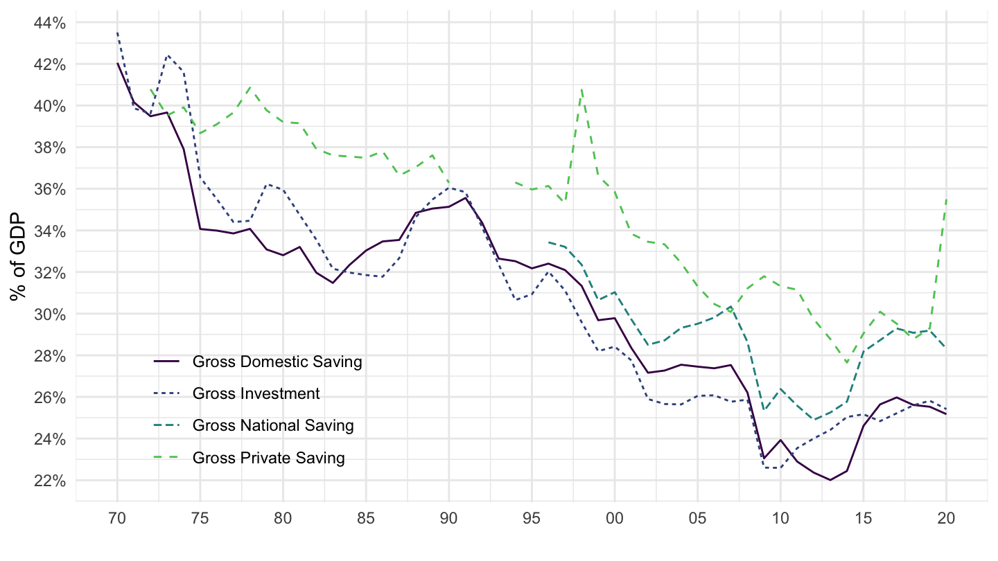

Germany

Code

NY.GDS.TOTL.ZS |>
  left_join(GC.NLD.TOTL.GD.ZS |> select(iso2c, year, GC.NLD.TOTL.GD.ZS = value), by = c("iso2c", "year")) |>
  left_join(NY.GNS.ICTR.ZS |> select(iso2c, year, NY.GNS.ICTR.ZS = value), by = c("iso2c", "year")) |>
  left_join(NE.GDI.TOTL.ZS |> select(iso2c, year, NE.GDI.TOTL.ZS = value), by = c("iso2c", "year")) |>
  rename(`Gross Domestic Saving` = value,
         `Gross National Saving` = NY.GNS.ICTR.ZS,
         `Public Saving` = GC.NLD.TOTL.GD.ZS,
         `Gross Investment` = NE.GDI.TOTL.ZS) |>
  mutate(`Gross Private Saving` = `Gross Domestic Saving` - `Public Saving`) |>
  select(-`Public Saving`) |>
  select(-iso3c, -variable) |>
  gather(variable, value, -iso2c, -year) |>
  filter(iso2c %in% c("DE")) |>
  left_join(iso2c, by = "iso2c") |>
  year_to_date() |>
  ggplot() + xlab("") + ylab("% of GDP") + theme_minimal() +
  geom_line(aes(x = date, y = value/100, color = variable, linetype = variable)) + 
  scale_color_manual(values = viridis(5)[1:4]) +
  theme(legend.title = element_blank(),
        legend.position = c(0.3, 0.85)) +
  scale_x_date(breaks = seq(1950, 2100, 5) |> paste0("-01-01") |> as.Date(),
               labels = date_format("%Y")) +
  scale_y_continuous(breaks = 0.01*seq(-60, 60, 2),
                     labels = scales::percent_format(accuracy = 1))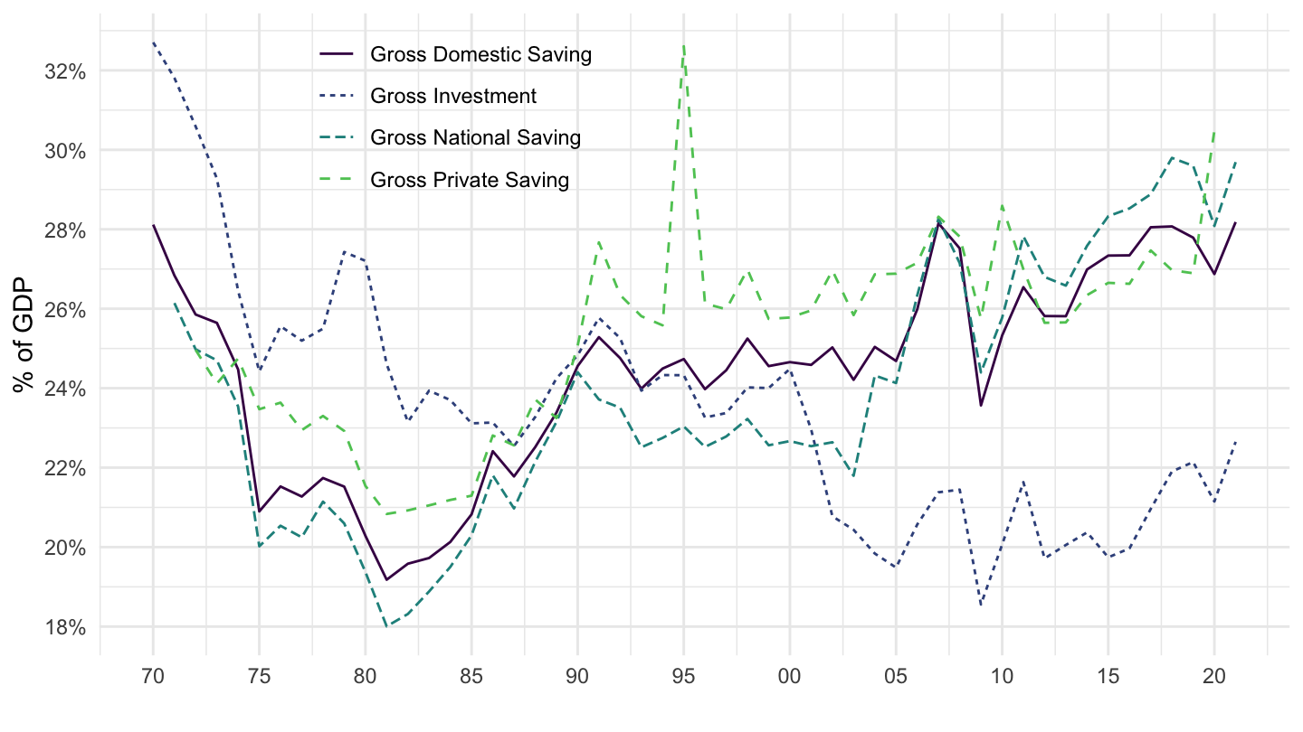

France

Code

NY.GDS.TOTL.ZS |>
  left_join(GC.NLD.TOTL.GD.ZS |> select(iso2c, year, GC.NLD.TOTL.GD.ZS = value), by = c("iso2c", "year")) |>
  left_join(NY.GNS.ICTR.ZS |> select(iso2c, year, NY.GNS.ICTR.ZS = value), by = c("iso2c", "year")) |>
  left_join(NE.GDI.TOTL.ZS |> select(iso2c, year, NE.GDI.TOTL.ZS = value), by = c("iso2c", "year")) |>
  rename(`Gross Domestic Saving` = value,
         `Gross National Saving` = NY.GNS.ICTR.ZS,
         `Public Saving` = GC.NLD.TOTL.GD.ZS,
         `Gross Investment` = NE.GDI.TOTL.ZS) |>
  mutate(`Gross Private Saving` = `Gross Domestic Saving` - `Public Saving`) |>
  select(-`Public Saving`) |>
  select(-iso3c, -variable) |>
  gather(variable, value, -iso2c, -year) |>
  filter(iso2c %in% c("FR")) |>
  left_join(iso2c, by = "iso2c") |>
  year_to_date() |>
  ggplot() + xlab("") + ylab("% of GDP") + theme_minimal() +
  geom_line(aes(x = date, y = value/100, color = variable, linetype = variable)) + 
  scale_color_manual(values = viridis(5)[1:4]) +
  theme(legend.title = element_blank(),
        legend.position = c(0.2, 0.2)) +
  scale_x_date(breaks = seq(1950, 2100, 5) |> paste0("-01-01") |> as.Date(),
               labels = date_format("%Y")) +
  scale_y_continuous(breaks = 0.01*seq(-60, 60, 2),
                     labels = scales::percent_format(accuracy = 1))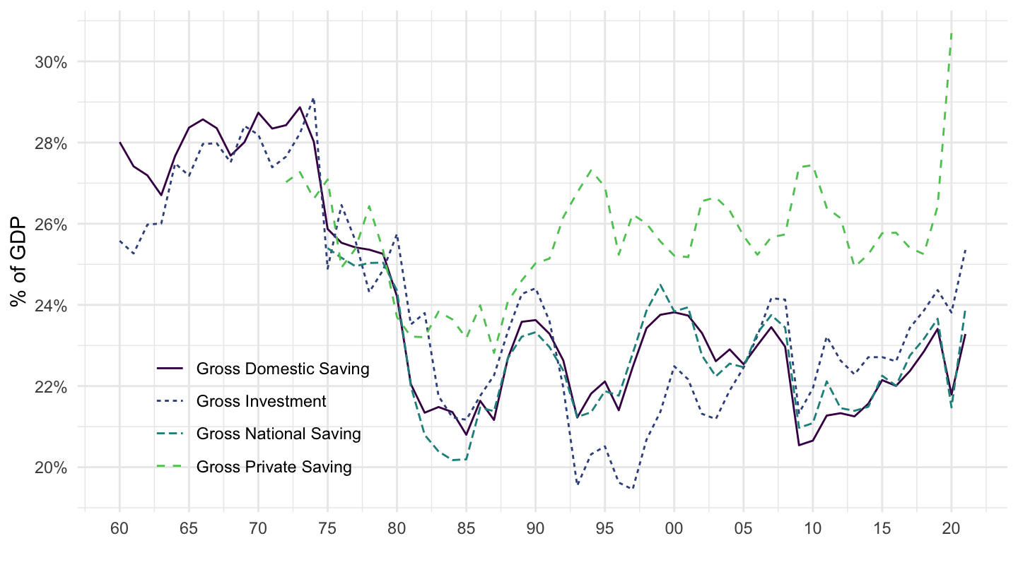

China

Code

NY.GDS.TOTL.ZS |>
  left_join(GC.NLD.TOTL.GD.ZS |> select(iso2c, year, GC.NLD.TOTL.GD.ZS = value), by = c("iso2c", "year")) |>
  rename(`Gross Domestic Saving` = value, `Public Saving` = GC.NLD.TOTL.GD.ZS) |>
  mutate(`Gross Private Saving` = `Gross Domestic Saving` + `Public Saving`) |>
  select(-iso3c, -variable) |>
  gather(variable, value, -iso2c, -year) |>
  filter(iso2c %in% c("CN")) |>
  left_join(iso2c, by = "iso2c") |>
  year_to_date() |>
  ggplot() + xlab("") + ylab("% of GDP") + theme_minimal() +
  geom_line(aes(x = date, y = value/100, color = variable, linetype = variable)) + 
  scale_color_manual(values = viridis(5)[1:4]) +
  theme(legend.title = element_blank(),
        legend.position = c(0.2, 0.55)) +
  scale_x_date(breaks = seq(1950, 2100, 5) |> paste0("-01-01") |> as.Date(),
               labels = date_format("%Y")) +
  scale_y_continuous(breaks = 0.01*seq(-60, 60, 2),
                     labels = scales::percent_format(accuracy = 1))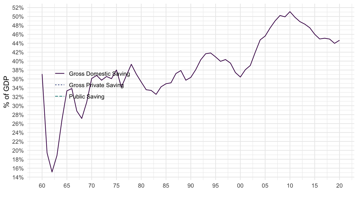

China, France, Germany

Code

NY.GDS.TOTL.ZS |>
  filter(iso2c %in% c("CN", "FR", "DE")) |>
  left_join(iso2c, by = "iso2c") |>
  year_to_date() |>
  mutate(value = value/100) |>
  add_flag_color("Iso2c") |>
  ggplot() + 
  geom_line(aes(x = date, y = value, color = color)) + 
  theme_minimal() + scale_color_identity() + add_flags +
  theme(legend.title = element_blank(),
        legend.position = c(0.1, 0.85)) +
  scale_x_date(breaks = seq(1950, 2100, 5) |> paste0("-01-01") |> as.Date(),
               labels = date_format("%Y")) +
  scale_y_continuous(breaks = 0.01*seq(-60, 60, 2),
                     labels = scales::percent_format(accuracy = 1)) +
  xlab("") + ylab("Gross domestic savings (% of GDP)")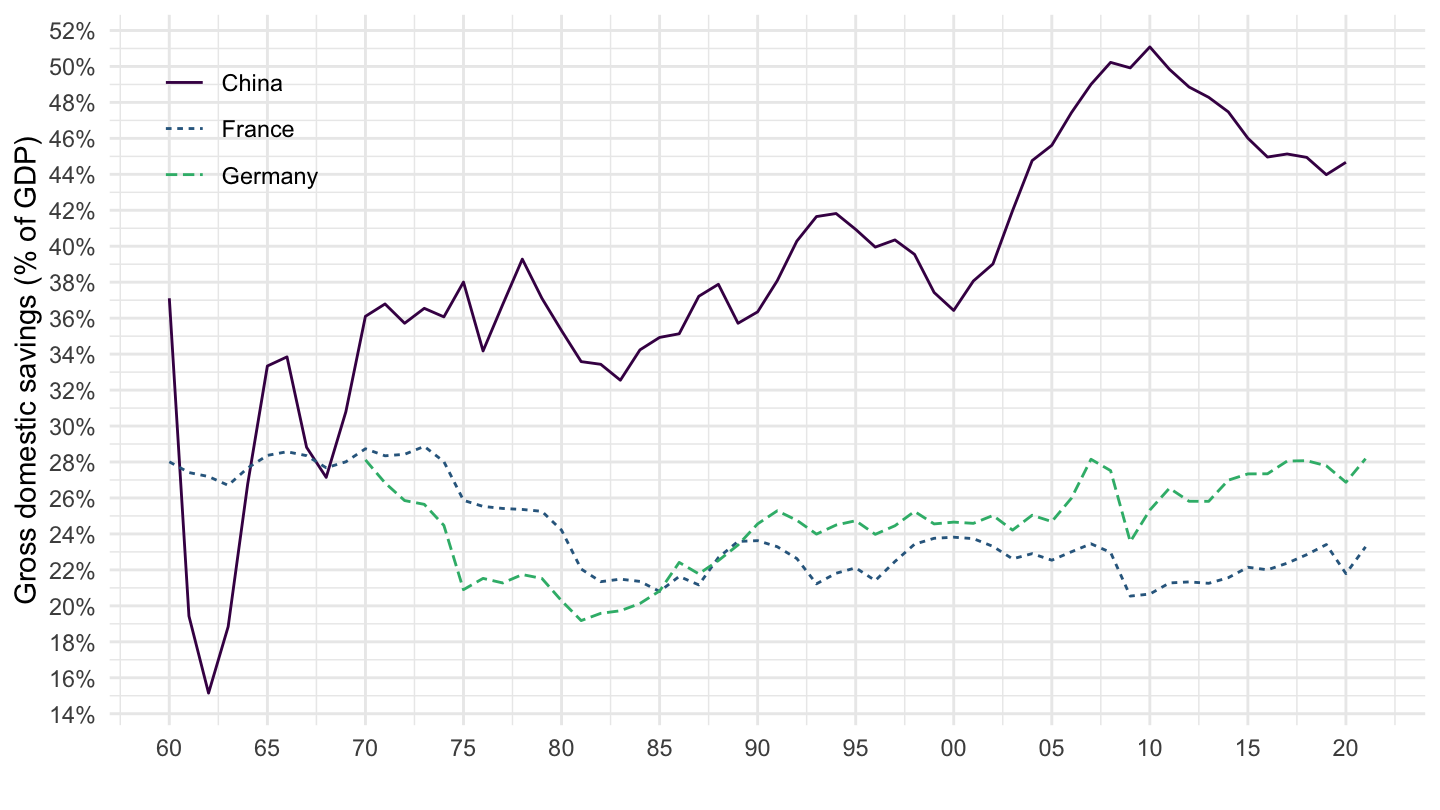

Spain, United Kingdom, United States

Code

NY.GDS.TOTL.ZS |>
  filter(iso2c %in% c("US", "GB", "ES")) |>
  left_join(iso2c, by = "iso2c") |>
  year_to_date() |>
  mutate(value = value/100) |>
  add_flag_color("Iso2c") |>
  ggplot() + 
  geom_line(aes(x = date, y = value, color = color)) + 
  theme_minimal() + scale_color_identity() + add_flags +
  theme(legend.title = element_blank(),
        legend.position = c(0.8, 0.9)) +
  scale_x_date(breaks = seq(1950, 2100, 5) |> paste0("-01-01") |> as.Date(),
               labels = date_format("%Y")) +
  scale_y_continuous(breaks = 0.01*seq(-60, 60, 2),
                     labels = scales::percent_format(accuracy = 1)) +
  xlab("") + ylab("Gross domestic savings (% of GDP)")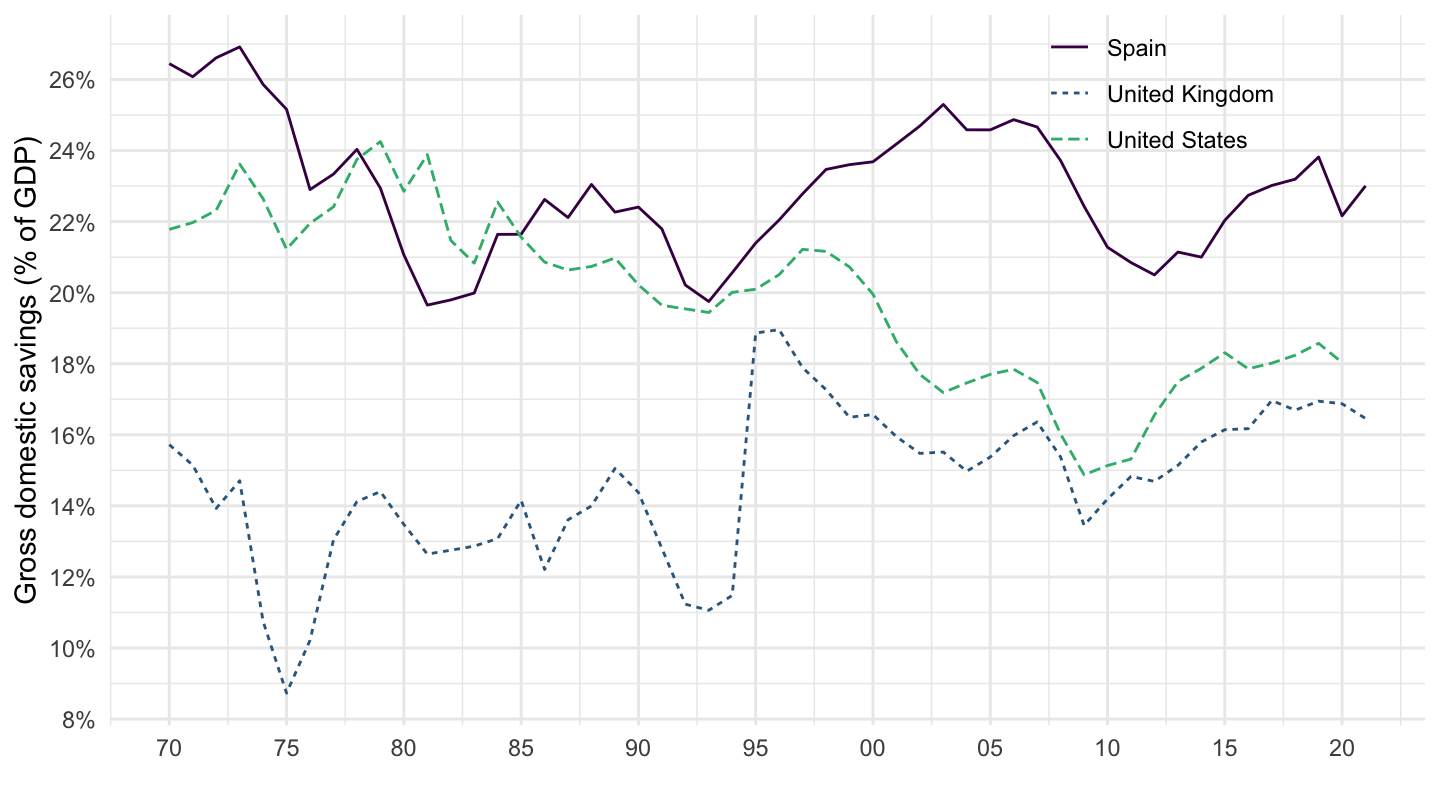

Argentina, Chile, Venezuela

Code

NY.GDS.TOTL.ZS |>
  filter(iso2c %in% c("AR", "CL", "VE")) |>
  left_join(iso2c, by = "iso2c") |>
  year_to_date() |>
  mutate(Iso2c = ifelse(iso2c == "VE", "Venezuela", Iso2c)) |>
  mutate(value = value/100) |>
  add_flag_color("Iso2c") |>
  ggplot() + 
  geom_line(aes(x = date, y = value, color = color)) + 
  theme_minimal() + scale_color_identity() + add_flags +
  theme(legend.title = element_blank(),
        legend.position = c(0.3, 0.9)) +
  scale_x_date(breaks = seq(1950, 2100, 5) |> paste0("-01-01") |> as.Date(),
               labels = date_format("%Y")) +
  scale_y_continuous(breaks = 0.01*seq(-60, 60, 5),
                     labels = scales::percent_format(accuracy = 1)) +
  xlab("") + ylab("Gross domestic savings (% of GDP)")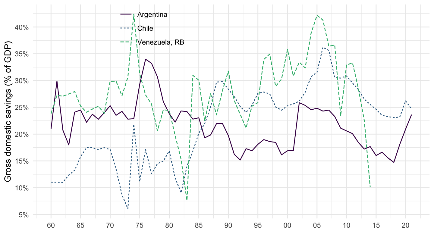

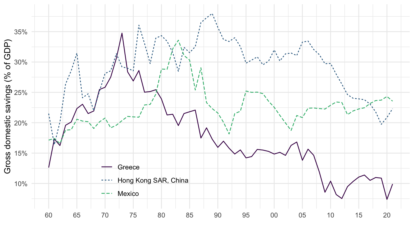
Greece, Hong Kong, Mexico

Code

NY.GDS.TOTL.ZS |>
  filter(iso2c %in% c("GR", "HK", "MX")) |>
  left_join(iso2c, by = "iso2c") |>
  year_to_date() |>
  mutate(Iso2c = ifelse(iso2c == "HK", "Hong Kong", Iso2c)) |>
  mutate(value = value/100) |>
  add_flag_color("Iso2c") |>
  ggplot() + 
  geom_line(aes(x = date, y = value, color = color)) + 
  theme_minimal() + scale_color_identity() + add_flags +
  theme(legend.title = element_blank(),
        legend.position = c(0.3, 0.15)) +
  scale_x_date(breaks = seq(1950, 2100, 5) |> paste0("-01-01") |> as.Date(),
               labels = date_format("%Y")) +
  scale_y_continuous(breaks = 0.01*seq(-60, 60, 5),
                     labels = scales::percent_format(accuracy = 1)) +
  xlab("") + ylab("Gross domestic savings (% of GDP)")