
Last observation: 2025 (N = 203)
First observation: 1970 (N = 144)
Last data update: 02 août 2026, 09:02
Last compile: 09 oct. 2026, 23:22
NAAG |>
  filter(REF_AREA %in% c("FRA", "ITA", "USA", "DEU"),
         INDICATOR == "DBTS13GDP") |>
  year_to_date() |>
  left_join(NAAG_var$LOCATION,  by = c("REF_AREA" = "LOCATION")) |>
  group_by(REF_AREA) |>
  arrange(date) |>
  select(date, REF_AREA, Location, obsValue) |>
  add_flag_color("Location") |>
  ggplot() + geom_line(aes(x = date, y = obsValue / 100, color = color)) +
  theme_minimal() + xlab("") + ylab("Gross debt of general government, % of GDP") +
  scale_color_identity() + add_4flags +
  scale_x_date(breaks = seq(1995, 2100, 5) |> paste0("-01-01") |> as.Date(),
               labels = date_format("%Y")) +
  scale_y_continuous(breaks = 0.01*seq(-10, 400, 10),
                     labels = percent_format(accuracy = 1)) +
  theme(legend.position = c(0.5, 0.90),
        legend.title = element_blank(),
        legend.direction = "horizontal")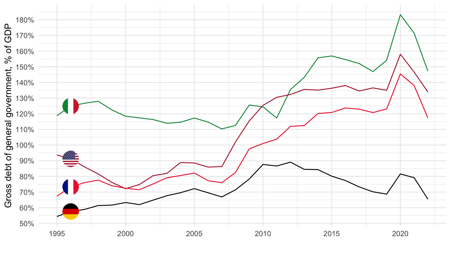
NAAG |>
  filter(INDICATOR == "B6NS14_S15DEF",
         REF_AREA %in% c("ITA", "ESP", "FRA", "DEU")) |>
  left_join(NAAG_var$LOCATION,  by = c("REF_AREA" = "LOCATION")) |>
  year_to_date() |>
  filter(date >= as.Date("1995-01-01")) |>
  select(Location, date, obsValue) |>
  add_flag_color("Location") |>
  group_by(Location) |>
  mutate(obsValue = 100*100*obsValue/obsValue[1]) |>
  ggplot() + geom_line(aes(x = date, y = obsValue/100, color = color)) +
  scale_color_identity() + add_4flags + theme_minimal() +
  scale_x_date(breaks = seq(1920, 2100, 5) |> paste0("-01-01") |> as.Date(),
               labels = date_format("%Y")) +
  scale_y_continuous(breaks = seq(100, 2000, 10)) +
  ylab("Real household net disposable income") + xlab("")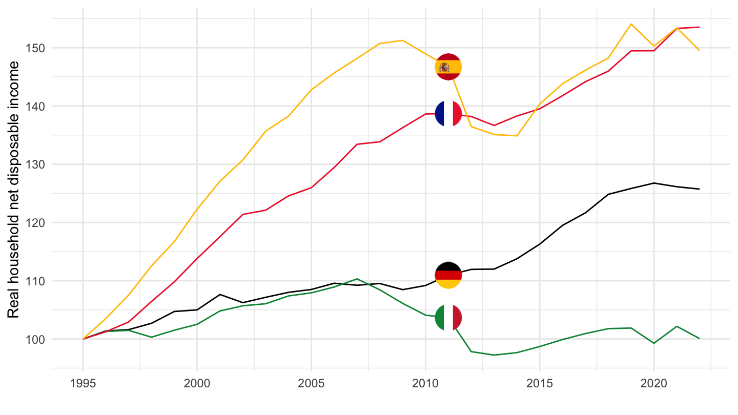
NAAG |>
  filter(INDICATOR == "B6NS14_S15DEF",
         REF_AREA %in% c("ITA", "ESP", "FRA", "DEU")) |>
  left_join(NAAG_var$LOCATION,  by = c("REF_AREA" = "LOCATION")) |>
  year_to_date() |>
  filter(date >= as.Date("1999-01-01")) |>
  select(Location, date, obsValue) |>
  add_flag_color("Location") |>
  group_by(Location) |>
  mutate(obsValue = 100*100*obsValue/obsValue[1]) |>
  ggplot() + geom_line(aes(x = date, y = obsValue/100, color = color)) +
  scale_color_identity() + add_4flags + theme_minimal() +
  scale_x_date(breaks = seq(1999, 2100, 5) |> paste0("-01-01") |> as.Date(),
               labels = date_format("%Y")) +
  scale_y_continuous(breaks = seq(10, 2000, 5)) +
  ylab("Real household net disposable income") + xlab("")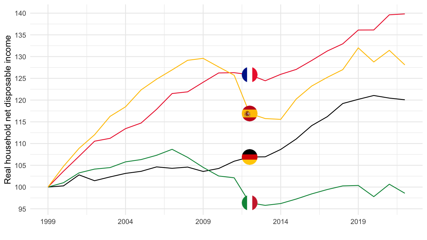
NAAG |>
  filter(INDICATOR == "B8NS14_S15SB6NS14",
         REF_AREA %in% c("ITA", "ESP", "FRA", "DEU")) |>
  left_join(NAAG_var$LOCATION,  by = c("REF_AREA" = "LOCATION")) |>
  year_to_date() |>
  select(Location, date, obsValue) |>
  add_flag_color("Location") |>
  ggplot() + geom_line(aes(x = date, y = obsValue / 100, color = color)) +
  scale_color_identity() + add_4flags + theme_minimal() +
  scale_x_date(breaks = seq(1920, 2100, 5) |> paste0("-01-01") |> as.Date(),
               labels = date_format("%Y")) +
  scale_y_continuous(breaks = 0.01*seq(-10, 40, 2),
                     labels = scales::percent_format(accuracy = 1)) +
  ylab("Net household saving (% of household NDI)") + xlab("")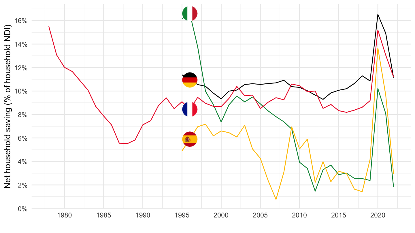
NAAG |>
  filter(INDICATOR == "B8NS",
         REF_AREA %in% c("AUT", "DNK", "NLD", "SWE", "DEU")) |>
  left_join(NAAG_var$LOCATION,  by = c("REF_AREA" = "LOCATION")) |>
  year_to_date() |>
  select(Location, date, obsValue) |>
  add_flag_color("Location") |>
  ggplot() + geom_line(aes(x = date, y = obsValue / 100, color = color)) +
  scale_color_identity() + add_5flags + theme_minimal() +
  scale_x_date(breaks = seq(1920, 2100, 5) |> paste0("-01-01") |> as.Date(),
               labels = date_format("%Y")) +
  scale_y_continuous(breaks = 0.01*seq(-10, 40, 2),
                     labels = scales::percent_format(accuracy = 1)) +
  ylab("Net Saving (% of GDP)") + xlab("")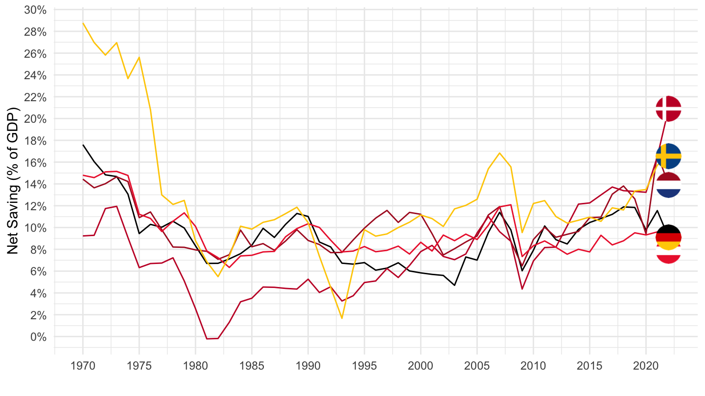
NAAG |>
  filter(INDICATOR == "B8NS",
         REF_AREA %in% c("AUT", "DNK", "NLD", "SWE")) |>
  left_join(NAAG_var$LOCATION,  by = c("REF_AREA" = "LOCATION")) |>
  year_to_date() |>
  select(Location, date, obsValue) |>
  add_flag_color("Location") |>
  ggplot() + geom_line(aes(x = date, y = obsValue / 100, color = color)) +
  scale_color_identity() + add_4flags + theme_minimal() +
  scale_x_date(breaks = seq(1920, 2100, 5) |> paste0("-01-01") |> as.Date(),
               labels = date_format("%Y")) +
  scale_y_continuous(breaks = 0.01*seq(-10, 40, 2),
                     labels = scales::percent_format(accuracy = 1)) +
  ylab("Net Saving (% of GDP)") + xlab("")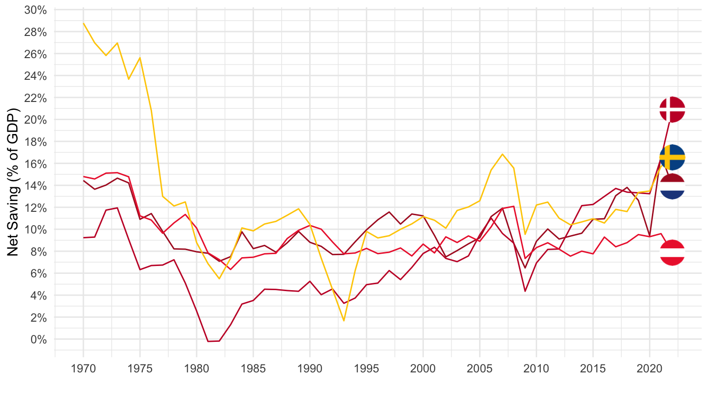
NAAG |>
  filter(INDICATOR == "B8NS",
         REF_AREA %in% c("ITA", "ESP", "FRA", "DEU")) |>
  left_join(NAAG_var$LOCATION,  by = c("REF_AREA" = "LOCATION")) |>
  year_to_date() |>
  select(Location, date, obsValue) |>
  add_flag_color("Location") |>
  ggplot() + geom_line(aes(x = date, y = obsValue / 100, color = color)) +
  scale_color_identity() + add_4flags + theme_minimal() +
  scale_x_date(breaks = seq(1920, 2100, 5) |> paste0("-01-01") |> as.Date(),
               labels = date_format("%Y")) +
  scale_y_continuous(breaks = 0.01*seq(-10, 40, 2),
                     labels = scales::percent_format(accuracy = 1)) +
  ylab("Net Saving (% of GDP)") + xlab("")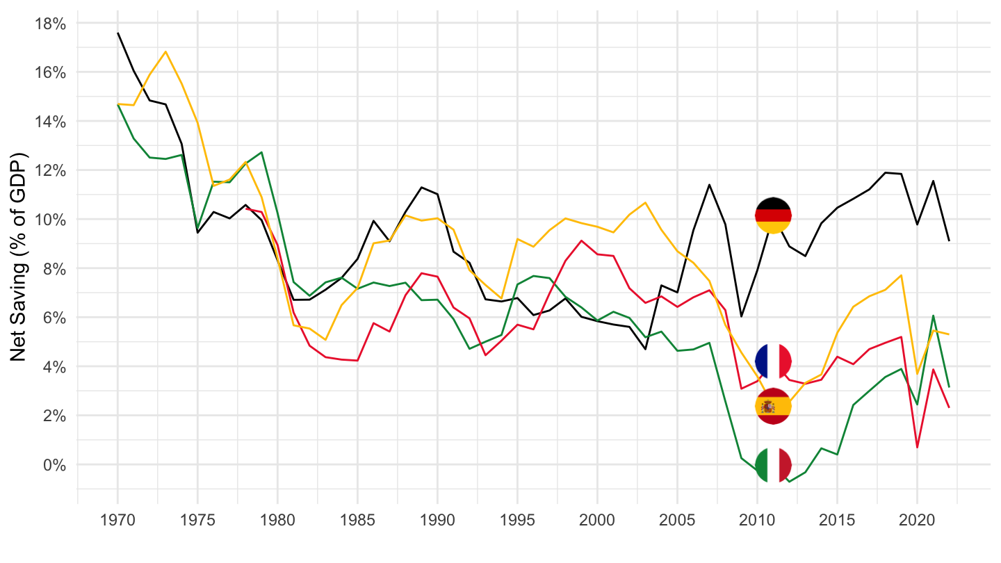
NAAG |>
  filter(INDICATOR == "B8NS13S",
         REF_AREA %in% c("AUT", "DNK", "NLD", "SWE", "DEU")) |>
  left_join(NAAG_var$LOCATION,  by = c("REF_AREA" = "LOCATION")) |>
  year_to_date() |>
  select(Location, date, obsValue) |>
  add_flag_color("Location") |>
  ggplot() + geom_line(aes(x = date, y = obsValue / 100, color = color)) +
  scale_color_identity() + add_5flags + theme_minimal() +
  scale_x_date(breaks = seq(1920, 2100, 2) |> paste0("-01-01") |> as.Date(),
               labels = date_format("%Y")) +
  scale_y_continuous(breaks = 0.01*seq(-10, 16, 1),
                     labels = scales::percent_format(accuracy = 0.1)) +
  ylab("Net Lending, General Government (% of GDP)") + xlab("")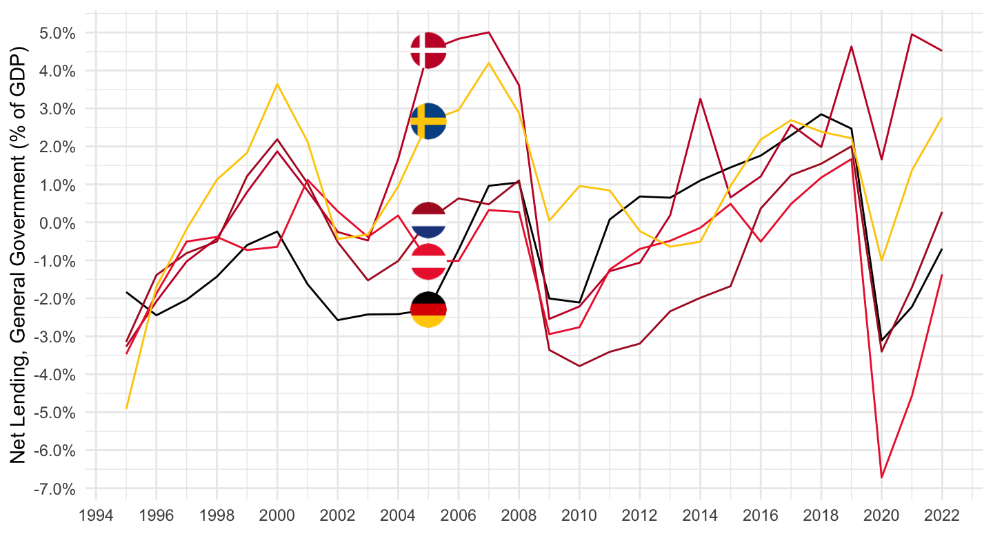
NAAG |>
  filter(INDICATOR == "B8NS13S",
         REF_AREA %in% c("AUT", "DNK", "NLD", "SWE")) |>
  left_join(NAAG_var$LOCATION,  by = c("REF_AREA" = "LOCATION")) |>
  year_to_date() |>
  select(Location, date, obsValue) |>
  add_flag_color("Location") |>
  ggplot() + geom_line(aes(x = date, y = obsValue / 100, color = color)) +
  scale_color_identity() + add_4flags + theme_minimal() +
  scale_x_date(breaks = seq(1920, 2100, 2) |> paste0("-01-01") |> as.Date(),
               labels = date_format("%Y")) +
  scale_y_continuous(breaks = 0.01*seq(-10, 16, 1),
                     labels = scales::percent_format(accuracy = 0.1)) +
  ylab("Net Lending, General Government (% of GDP)") + xlab("")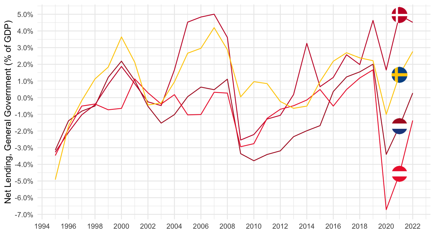
NAAG |>
  filter(INDICATOR == "B8NS13S",
         REF_AREA %in% c("ITA", "ESP", "FRA", "DEU")) |>
  left_join(NAAG_var$LOCATION,  by = c("REF_AREA" = "LOCATION")) |>
  year_to_date() |>
  select(Location, date, obsValue) |>
  add_flag_color("Location") |>
  ggplot() + geom_line(aes(x = date, y = obsValue / 100, color = color)) +
  scale_color_identity() + add_4flags + theme_minimal() +
  scale_x_date(breaks = seq(1920, 2100, 5) |> paste0("-01-01") |> as.Date(),
               labels = date_format("%Y")) +
  scale_y_continuous(breaks = 0.01*seq(-10, 16, 1),
                     labels = scales::percent_format(accuracy = 0.1)) +
  ylab("Net Lending, General Government (% of GDP)") + xlab("")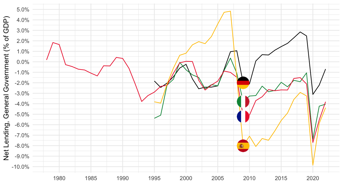
NAAG |>
  filter(REF_AREA %in% c("FRA", "ITA", "DEU", "PRT"),
         INDICATOR == "TOT") |>
  year_to_date() |>
  left_join(NAAG_var$LOCATION, by = c("REF_AREA" = "LOCATION")) |>
  add_flag_color("Location") |>
  ggplot() + geom_line(aes(x = date, y = obsValue / 100, color = color)) +
  theme_minimal() + xlab("") + ylab("Terms of Trade") +
  scale_color_identity() + add_4flags +
  scale_x_date(breaks = seq(1960, 2100, 5) |> paste0("-01-01") |> as.Date(),
               labels = date_format("%Y")) +
  scale_y_continuous(breaks = 0.01*seq(-10, 400, 10),
                     labels = percent_format(accuracy = 1)) +
  theme(legend.position = c(0.5, 0.90),
        legend.title = element_blank(),
        legend.direction = "horizontal")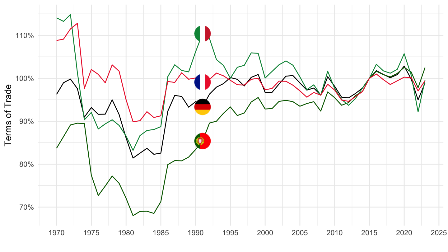
NAAG |>
  filter(REF_AREA %in% c("FRA", "ITA", "DEU", "PRT"),
         INDICATOR == "DBTS14_S15NDI") |>
  year_to_date() |>
  left_join(NAAG_var$LOCATION,  by = c("REF_AREA" = "LOCATION")) |>
  group_by(REF_AREA) |>
  arrange(date) |>
  select(date, REF_AREA, Location, obsValue) |>
  add_flag_color("Location") |>
  ggplot() + geom_line(aes(x = date, y = obsValue / 100, color = color)) +
  theme_minimal() + xlab("") + ylab("Household Debt, % of NDI") +
  scale_color_identity() + add_4flags +
  scale_x_date(breaks = seq(1960, 2100, 2) |> paste0("-01-01") |> as.Date(),
               labels = date_format("%Y")) +
  scale_y_continuous(breaks = 0.01*seq(-10, 400, 10),
                     labels = percent_format(accuracy = 1)) +
  theme(legend.position = c(0.5, 0.90),
        legend.title = element_blank(),
        legend.direction = "horizontal")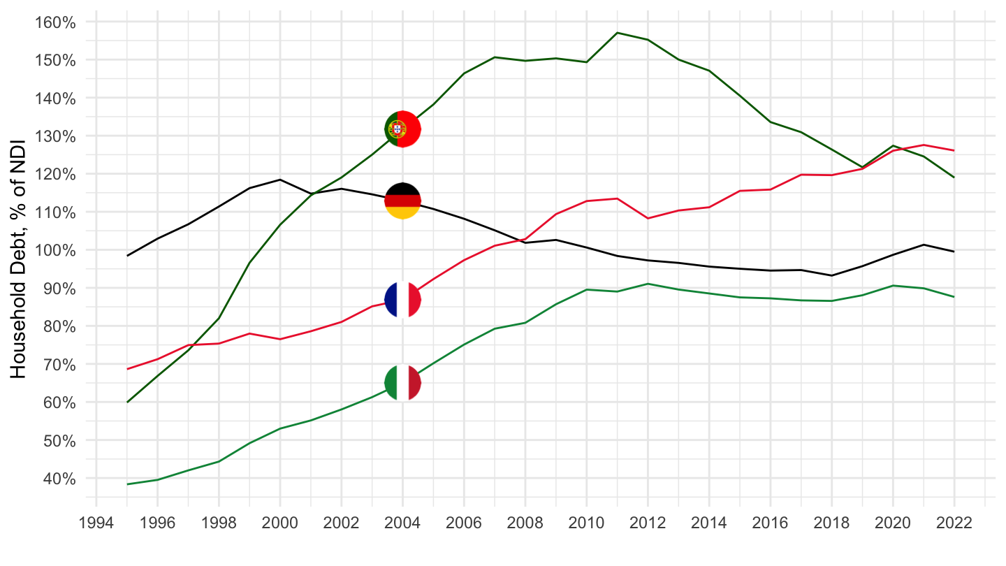
NAAG |>
  year_to_date() |>
  filter(REF_AREA %in% c("FRA", "ITA", "DEU", "PRT"),
         INDICATOR == "DBTS14_S15NDI",
         date >= as.Date("2008-01-01")) |>
  left_join(NAAG_var$LOCATION,  by = c("REF_AREA" = "LOCATION")) |>
  group_by(REF_AREA) |>
  arrange(date) |>
  select(date, REF_AREA, Location, obsValue) |>
  add_flag_color("Location") |>
  ggplot() + geom_line(aes(x = date, y = obsValue / 100, color = color)) +
  scale_color_identity() + add_4flags +
  theme_minimal() + xlab("") + ylab("Household Debt, % of NDI") +
  scale_x_date(breaks = seq(1960, 2100, 1) |> paste0("-01-01") |> as.Date(),
               labels = date_format("%Y")) +
  scale_y_continuous(breaks = 0.01*seq(-10, 400, 10),
                     labels = percent_format(accuracy = 1)) +
  theme(legend.position = c(0.5, 0.90),
        legend.title = element_blank(),
        legend.direction = "horizontal")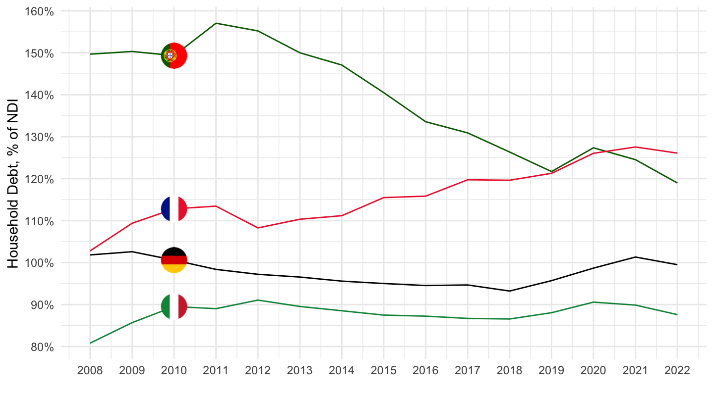
(ref:B8NS-FRA-DEU) Net saving , TOTAL (% of GDP)
NAAG |>
  filter(INDICATOR == "B8NS",
         REF_AREA %in% c("FRA", "DEU")) |>
  left_join(NAAG_var$LOCATION,  by = c("REF_AREA" = "LOCATION")) |>
  left_join(NAAG_var$INDICATOR,  by = "INDICATOR") |>
  year_to_date() |>
  arrange(Location) |>
  select(Indicator, Location, date, obsValue) |>
  add_flag_color("Location") |>
  ggplot() + geom_line(aes(x = date, y = obsValue / 100, color = color)) +
  scale_color_identity() + add_2flags + theme_minimal() +
  scale_x_date(breaks = seq(1920, 2100, 5) |> paste0("-01-01") |> as.Date(),
               labels = date_format("%Y")) +
  scale_y_continuous(breaks = 0.01*seq(-7, 30, 2),
                     labels = scales::percent_format(accuracy = 0.1)) +
  ylab("Net Saving, Total (% of GDP)") + xlab("")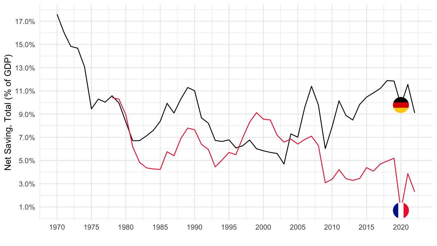
(ref:B8NS13S-FRA-DEU) Net saving of General Government (% of GDP)
NAAG |>
  filter(INDICATOR == "B8NS13S",
         REF_AREA %in% c("FRA", "DEU")) |>
  left_join(NAAG_var$LOCATION,  by = c("REF_AREA" = "LOCATION")) |>
  left_join(NAAG_var$INDICATOR,  by = "INDICATOR") |>
  year_to_date() |>
  filter(year(date) >= 1990) |>
  arrange(Location) |>
  select(Indicator, Location, date, obsValue) |>
  add_flag_color("Location") |>
  ggplot() + geom_line(aes(x = date, y = obsValue / 100, color = color)) +
  scale_color_identity() + add_2flags + theme_minimal() +
  scale_x_date(breaks = seq(1920, 2100, 2) |> paste0("-01-01") |> as.Date(),
               labels = date_format("%Y")) +
  theme(legend.position = c(0.1, 0.9),
        legend.title = element_blank()) +
  scale_y_continuous(breaks = 0.01*seq(-7, 16, 0.5),
                     labels = scales::percent_format(accuracy = 0.1)) +
  ylab("Net Lending, General Government (% of GDP)") + xlab("")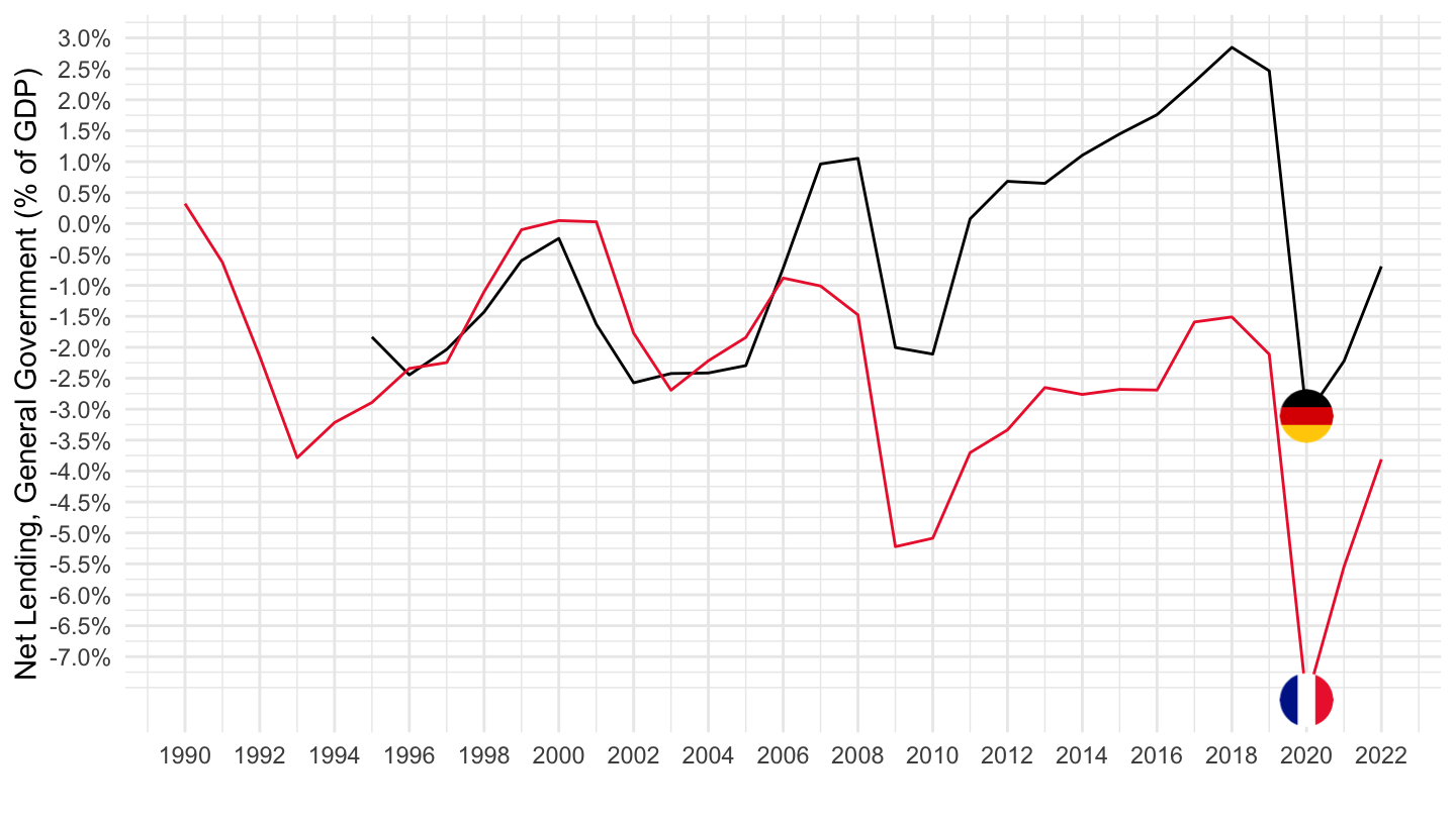
(ref:B9S14-S15S-FRA-DEU) Corporate Saving
NAAG |>
  filter(INDICATOR == "B9S14_S15S",
         REF_AREA %in% c("FRA", "DEU")) |>
  left_join(NAAG_var$LOCATION,  by = c("REF_AREA" = "LOCATION")) |>
  left_join(NAAG_var$INDICATOR,  by = "INDICATOR") |>
  year_to_date() |>
  filter(year(date) >= 1990) |>
  arrange(Location) |>
  select(Indicator, Location, date, obsValue) |>
  add_flag_color("Location") |>
  ggplot() + geom_line(aes(x = date, y = obsValue / 100, color = color)) +
  scale_color_identity() + add_2flags + theme_minimal() +
  scale_x_date(breaks = seq(1920, 2100, 2) |> paste0("-01-01") |> as.Date(),
               labels = date_format("%Y")) +
  theme(legend.position = c(0.1, 0.9),
        legend.title = element_blank()) +
  scale_y_continuous(breaks = 0.01*seq(-7, 16, 0.5),
                     labels = scales::percent_format(accuracy = 0.1)) +
  ylab("Net lending/net borrowing, Households and NPISHs") + xlab("")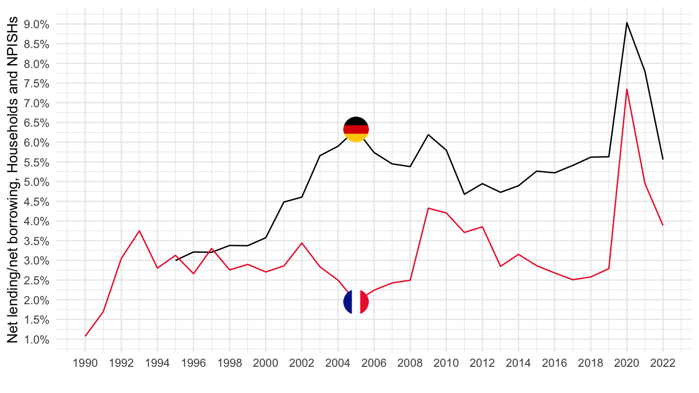
(ref:B9S1S-FRA-DEU) Net lending/net borrowing, Total economy
NAAG |>
  filter(INDICATOR == "B9S1S",
         REF_AREA %in% c("FRA", "DEU")) |>
  left_join(NAAG_var$LOCATION,  by = c("REF_AREA" = "LOCATION")) |>
  left_join(NAAG_var$INDICATOR,  by = "INDICATOR") |>
  year_to_date() |>
  filter(year(date) >= 1990) |>
  arrange(Location) |>
  select(Indicator, Location, date, obsValue) |>
  add_flag_color("Location") |>
  ggplot() + geom_line(aes(x = date, y = obsValue / 100, color = color)) +
  scale_color_identity() + add_2flags + theme_minimal() +
  scale_x_date(breaks = seq(1920, 2100, 2) |> paste0("-01-01") |> as.Date(),
               labels = date_format("%Y")) +
  theme(legend.position = c(0.1, 0.9),
        legend.title = element_blank()) +
  scale_y_continuous(breaks = 0.01*seq(-7, 16, 0.5),
                     labels = scales::percent_format(accuracy = 0.1)) +
  ylab("% of GDP") + xlab("")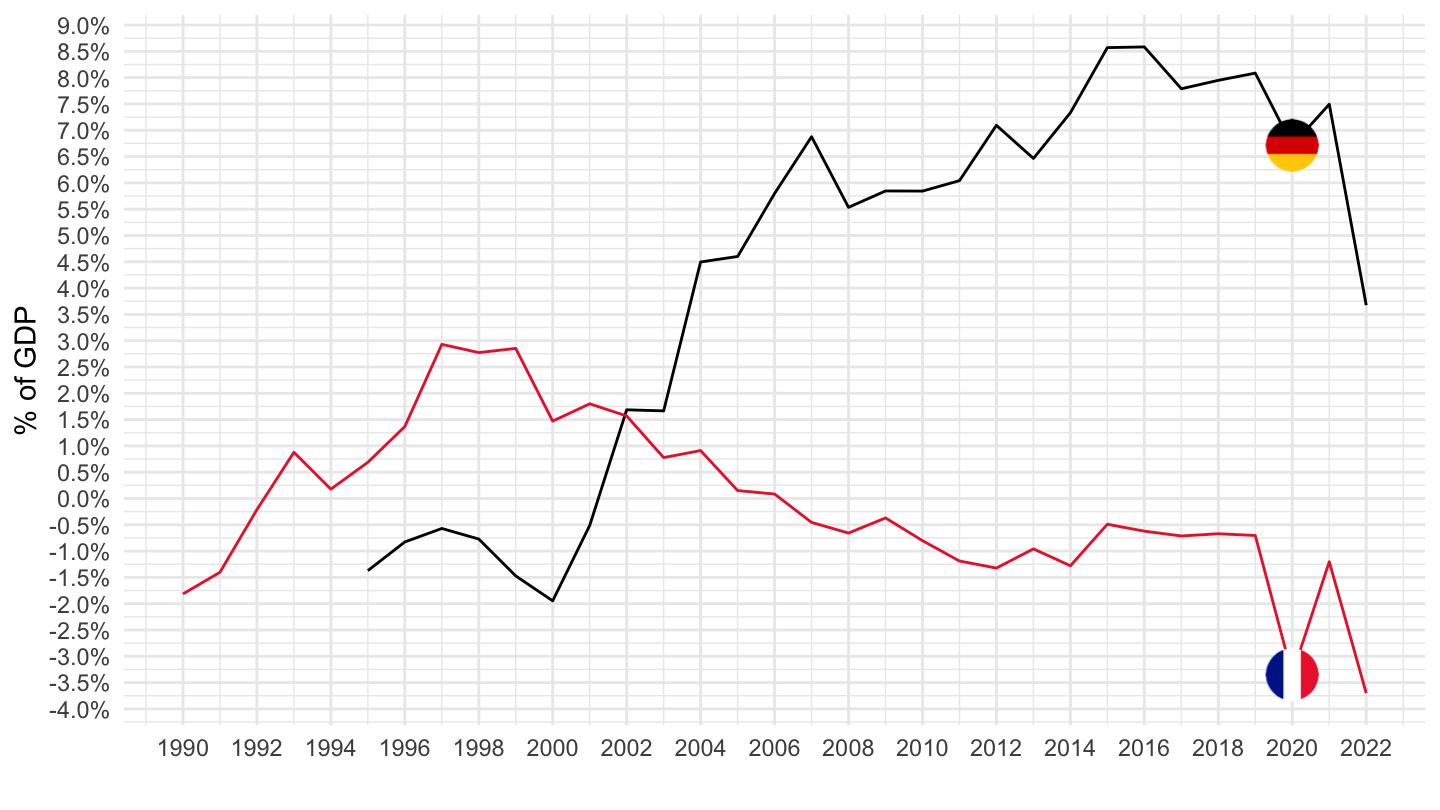
(ref:B9S11-S12S-FRA-DEU) Net lending/net borrowing, Corporations
NAAG |>
  filter(INDICATOR == "B9S11_S12S",
         REF_AREA %in% c("FRA", "DEU")) |>
  left_join(NAAG_var$LOCATION,  by = c("REF_AREA" = "LOCATION")) |>
  left_join(NAAG_var$INDICATOR,  by = "INDICATOR") |>
  year_to_date() |>
  filter(year(date) >= 1990) |>
  arrange(Location) |>
  select(Indicator, Location, date, obsValue) |>
  add_flag_color("Location") |>
  ggplot() + geom_line(aes(x = date, y = obsValue / 100, color = color)) +
  scale_color_identity() + add_2flags + theme_minimal() +
  scale_x_date(breaks = seq(1920, 2100, 2) |> paste0("-01-01") |> as.Date(),
               labels = date_format("%Y")) +
  theme(legend.position = c(0.1, 0.9),
        legend.title = element_blank()) +
  scale_y_continuous(breaks = 0.01*seq(-7, 16, 0.5),
                     labels = scales::percent_format(accuracy = 0.1)) +
  ylab("% of GDP") + xlab("")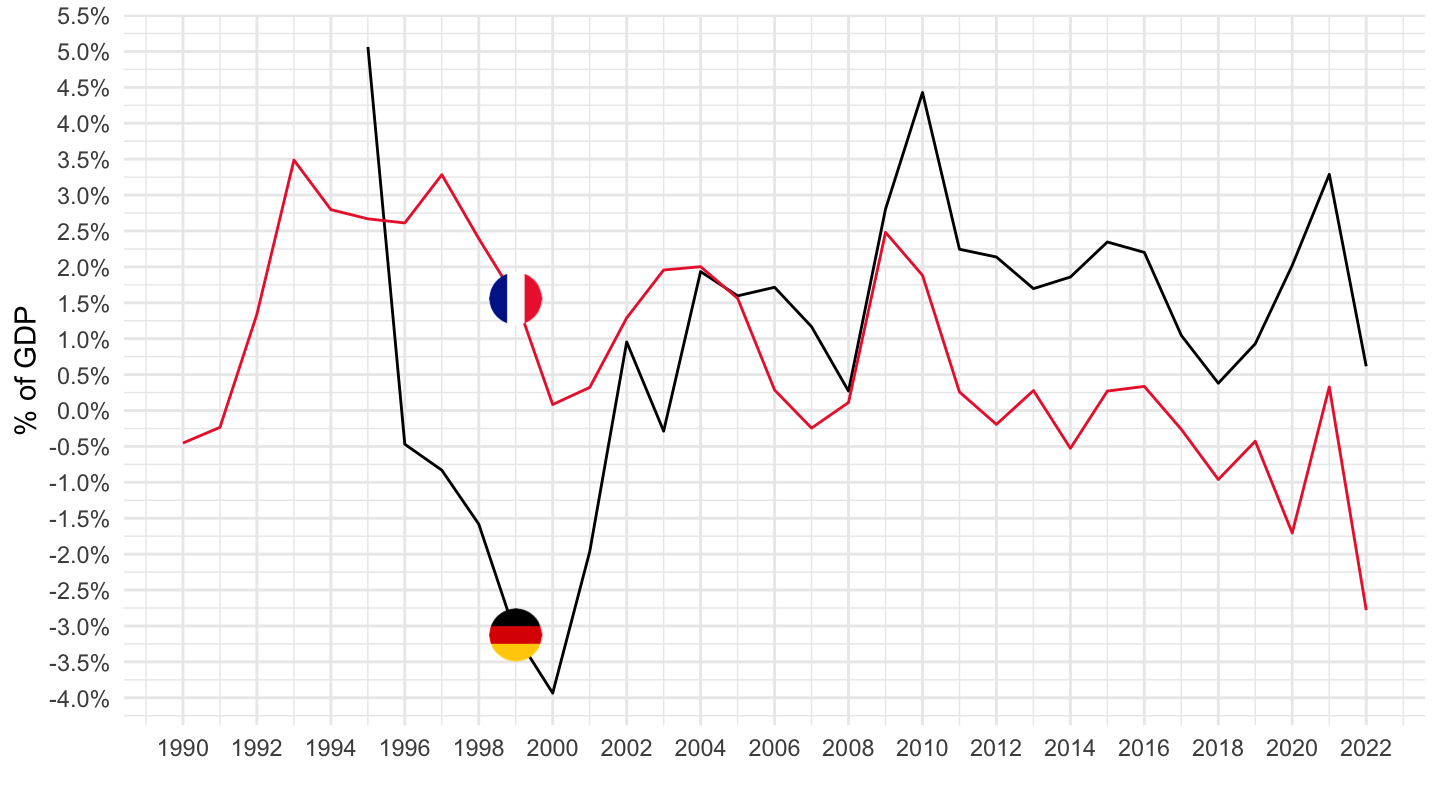
NAAG |>
  filter(INDICATOR == "TOTNETWORTHS14_S15NDI",
         REF_AREA %in% c("FRA", "DEU")) |>
  left_join(NAAG_var$LOCATION,  by = c("REF_AREA" = "LOCATION")) |>
  left_join(NAAG_var$INDICATOR,  by = "INDICATOR") |>
  year_to_date() |>
  filter(year(date) >= 1990) |>
  arrange(Location) |>
  select(Indicator, Location, date, obsValue) |>
  add_flag_color("Location") |>
  ggplot() + geom_line(aes(x = date, y = obsValue / 100, color = color)) +
  scale_color_identity() + add_2flags + theme_minimal() +
  scale_x_date(breaks = seq(1920, 2100, 2) |> paste0("-01-01") |> as.Date(),
               labels = date_format("%Y")) +
  theme(legend.position = c(0.1, 0.9),
        legend.title = element_blank()) +
  scale_y_continuous(breaks = 0.01*seq(0, 900, 20),
                     labels = scales::percent_format(accuracy = 1)) +
  ylab("% of Disposable Income") + xlab("")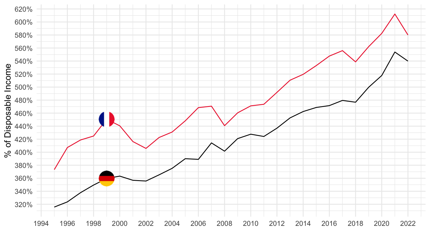
NAAG |>
  filter(INDICATOR == "P040B7NS14_S15",
         REF_AREA %in% c("FRA", "DEU")) |>
  left_join(NAAG_var$LOCATION,  by = c("REF_AREA" = "LOCATION")) |>
  left_join(NAAG_var$INDICATOR,  by = "INDICATOR") |>
  year_to_date() |>
  filter(year(date) >= 1990) |>
  arrange(Location) |>
  select(Indicator, Location, date, obsValue) |>
  add_flag_color("Location") |>
  ggplot() + geom_line(aes(x = date, y = obsValue / 100, color = color)) +
  scale_color_identity() + add_2flags + theme_minimal() +
  scale_x_date(breaks = seq(1920, 2100, 2) |> paste0("-01-01") |> as.Date(),
               labels = date_format("%Y")) +
  theme(legend.position = c(0.1, 0.9),
        legend.title = element_blank()) +
  scale_y_continuous(breaks = 0.01*seq(-7, 25, 0.5),
                     labels = scales::percent_format(accuracy = 0.1)) +
  ylab("% of GDP") + xlab("")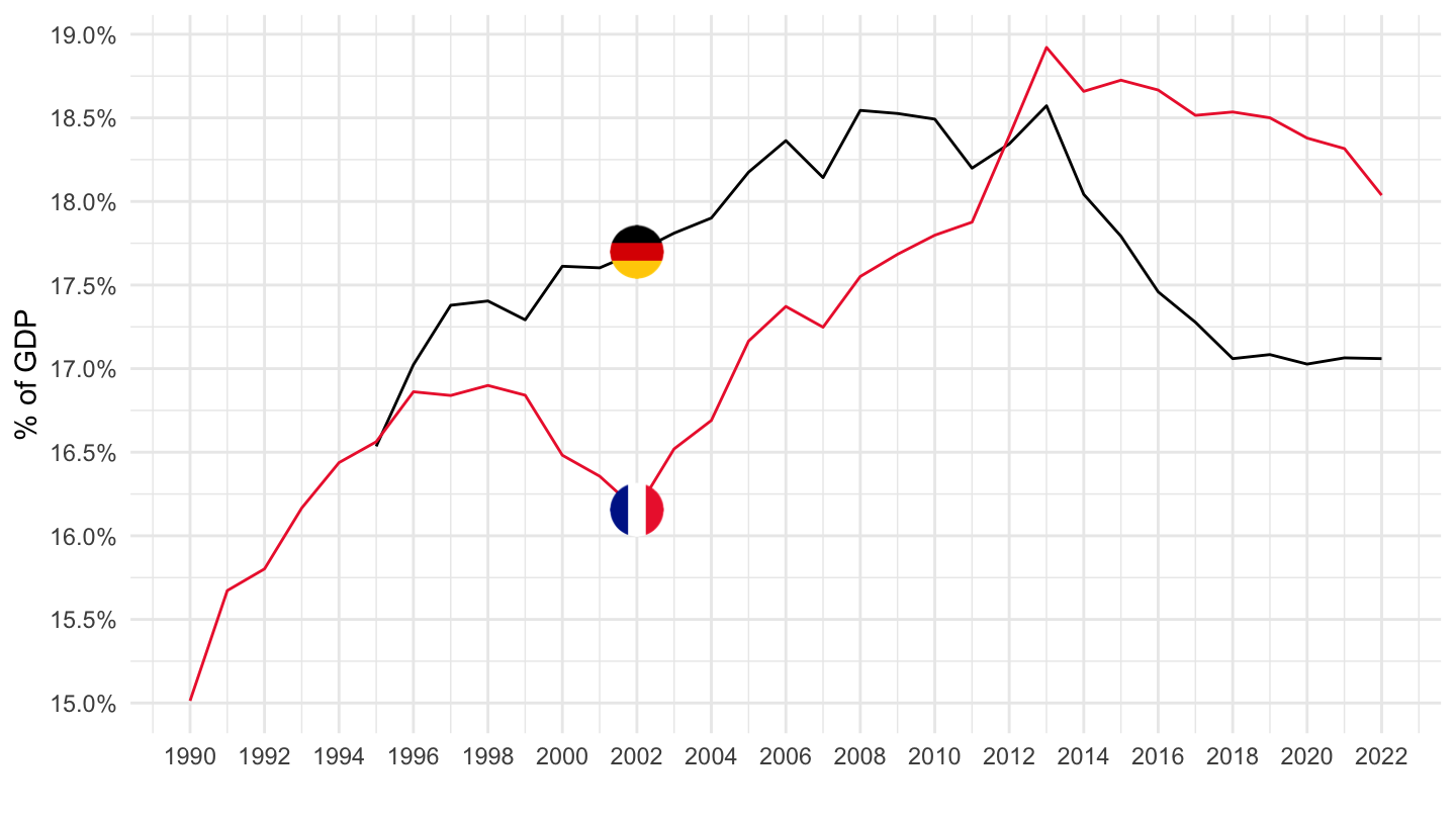
NAAG |>
  filter(INDICATOR == "B8NS14_S15SB6NS14",
         REF_AREA %in% c("FRA", "DEU")) |>
  left_join(NAAG_var$LOCATION,  by = c("REF_AREA" = "LOCATION")) |>
  left_join(NAAG_var$INDICATOR,  by = "INDICATOR") |>
  year_to_date() |>
  filter(year(date) >= 1990) |>
  arrange(Location) |>
  select(Indicator, Location, date, obsValue) |>
  add_flag_color("Location") |>
  ggplot() + geom_line(aes(x = date, y = obsValue / 100, color = color)) +
  scale_color_identity() + add_2flags + theme_minimal() +
  scale_x_date(breaks = seq(1920, 2100, 2) |> paste0("-01-01") |> as.Date(),
               labels = date_format("%Y")) +
  theme(legend.position = c(0.1, 0.9),
        legend.title = element_blank()) +
  scale_y_continuous(breaks = 0.01*seq(-7, 16, 0.5),
                     labels = scales::percent_format(accuracy = 0.1)) +
  ylab("% of GDP") + xlab("")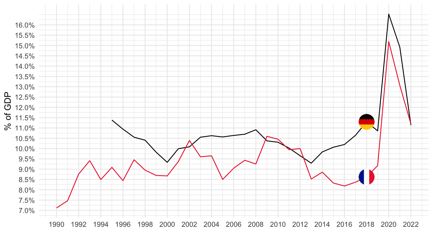
nber_recessions_extract <- nber_recessions |>
  filter(Peak >= as.Date("1970-01-01"))
NAAG |>
  filter(REF_AREA %in% c("FRA", "USA", "DEU", "JPN"),
         INDICATOR == "B8NS") |>
  year_to_date() |>
  left_join(NAAG_var$LOCATION,  by = c("REF_AREA" = "LOCATION")) |>
  group_by(REF_AREA) |>
  arrange(date) |>
  add_flag_color("Location") |>
  ggplot() + geom_line(aes(x = date, y = obsValue / 100, color = color)) +
  scale_color_identity() + add_4flags +
  theme_minimal() + xlab("") + ylab("Net saving rate, % of GDP") +
  geom_rect(data = nber_recessions_extract,
            aes(xmin = Peak, xmax = Trough, ymin = -Inf, ymax = +Inf),
            fill = 'grey', alpha = 0.5) +
  scale_x_date(breaks = seq(1960, 2100, 5) |> paste0("-01-01") |> as.Date(),
               labels = date_format("%Y")) +
  scale_y_continuous(breaks = 0.01*seq(-10, 50, 2),
                     labels = percent_format(accuracy = 1))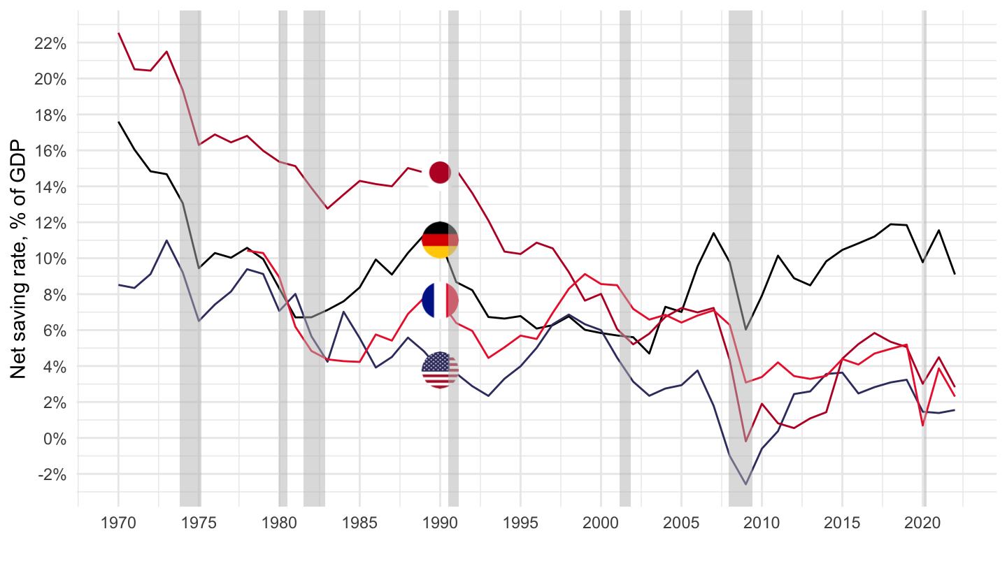
nber_recessions_extract <- nber_recessions |>
  filter(Peak >= as.Date("1970-01-01"))
NAAG |>
  filter(REF_AREA %in% c("FRA", "USA", "DEU", "JPN"),
         INDICATOR == "B8NS13S") |>
  year_to_date() |>
  left_join(NAAG_var$LOCATION,  by = c("REF_AREA" = "LOCATION")) |>
  group_by(REF_AREA) |>
  arrange(date) |>
  add_flag_color("Location") |>
  ggplot() + geom_line(aes(x = date, y = obsValue / 100, color = color)) +
  scale_color_identity() + add_4flags +
  theme_minimal() + xlab("") + ylab("Net saving of General Government, % of GDP") +
  geom_rect(data = nber_recessions_extract,
            aes(xmin = Peak, xmax = Trough, ymin = -Inf, ymax = +Inf),
            fill = 'grey', alpha = 0.5) +
  scale_x_date(breaks = seq(1960, 2100, 5) |> paste0("-01-01") |> as.Date(),
               labels = date_format("%Y")) +
  scale_y_continuous(breaks = 0.01*seq(-20, 50, 1),
                     labels = percent_format(accuracy = 1)) +
  theme(legend.position = c(0.4, 0.15),
        legend.title = element_blank(),
        legend.direction = "horizontal")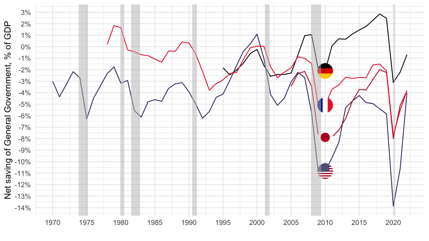
nber_recessions_extract <- nber_recessions |>
  filter(Peak >= as.Date("1970-01-01"))
NAAG |>
  filter(REF_AREA %in% c("FRA", "USA", "DEU", "JPN"),
         INDICATOR == "B9S11_S12S") |>
  year_to_date() |>
  left_join(NAAG_var$LOCATION,  by = c("REF_AREA" = "LOCATION")) |>
  add_flag_color("Location") |>
  ggplot() + geom_line(aes(x = date, y = obsValue / 100, color = color)) +
  scale_color_identity() + add_4flags +
  theme_minimal() + xlab("") + ylab("Net lending, Corporations, % of GDP") +
  scale_x_date(breaks = seq(1960, 2100, 5) |> paste0("-01-01") |> as.Date(),
               labels = date_format("%Y")) +
  scale_y_continuous(breaks = 0.01*seq(-20, 50, 1),
                     labels = percent_format(accuracy = 1)) +
  geom_rect(data = nber_recessions_extract,
            aes(xmin = Peak, xmax = Trough, ymin = -Inf, ymax = +Inf),
            fill = 'grey', alpha = 0.5) +
  theme(legend.position = c(0.3, 0.90),
        legend.title = element_blank(),
        legend.direction = "horizontal")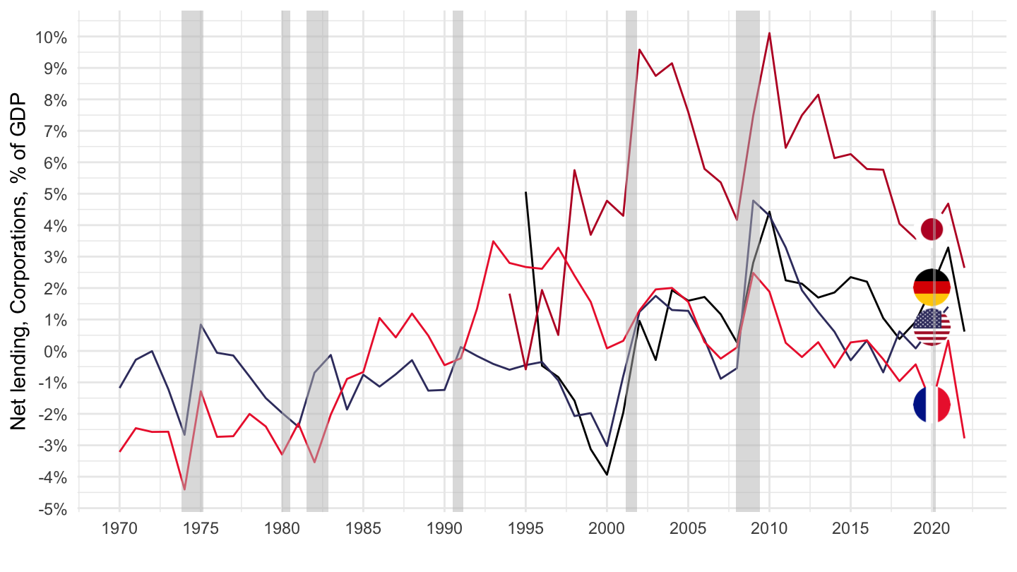
nber_recessions_extract <- nber_recessions |>
  filter(Peak >= as.Date("1970-01-01"))
NAAG |>
  filter(REF_AREA %in% c("FRA", "USA", "DEU", "JPN"),
         INDICATOR == "B8NS14_S15SB6NS14") |>
  year_to_date() |>
  left_join(NAAG_var$LOCATION,  by = c("REF_AREA" = "LOCATION")) |>
  add_flag_color("Location") |>
  ggplot() + geom_line(aes(x = date, y = obsValue / 100, color = color)) +
  scale_color_identity() + add_4flags +
  theme_minimal() + xlab("") + ylab("Net household saving, % of households NDI") +
  geom_rect(data = nber_recessions_extract,
            aes(xmin = Peak, xmax = Trough, ymin = -Inf, ymax = +Inf),
            fill = 'grey', alpha = 0.5) +
  scale_x_date(breaks = seq(1960, 2100, 5) |> paste0("-01-01") |> as.Date(),
               labels = date_format("%Y")) +
  scale_y_continuous(breaks = 0.01*seq(-20, 50, 1),
                     labels = percent_format(accuracy = 1)) +
  theme(legend.position = c(0.4, 0.10),
        legend.title = element_blank(),
        legend.direction = "horizontal")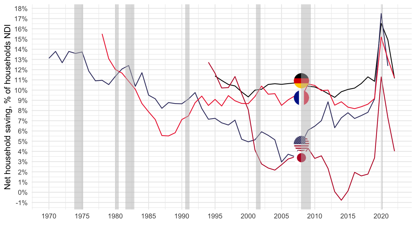
nber_recessions_extract <- nber_recessions |>
  filter(Peak >= as.Date("1970-01-01"))
NAAG |>
  filter(REF_AREA %in% c("FRA", "USA", "DEU", "JPN"),
         INDICATOR == "P51S") |>
  year_to_date() |>
  mutate(value = obsValue / 100) |>
  left_join(NAAG_var$LOCATION, by = c("REF_AREA" = "LOCATION")) |>
  add_flag_color("Location") |>
  ggplot() + geom_line(aes(x = date, y = obsValue / 100, color = color)) +
  scale_color_identity() + add_4flags +
  theme_minimal() + xlab("") + ylab("Gross fixed capital formation (% of GDP)") +
  geom_rect(data = nber_recessions_extract,
            aes(xmin = Peak, xmax = Trough, ymin = -Inf, ymax = +Inf),
            fill = 'grey', alpha = 0.5) +
  scale_x_date(breaks = seq(1960, 2100, 5) |> paste0("-01-01") |> as.Date(),
               labels = date_format("%Y")) +
  scale_y_continuous(breaks = 0.01*seq(-20, 50, 2),
                     labels = percent_format(accuracy = 1)) +
  theme(legend.position = c(0.8, 0.80),
        legend.title = element_blank())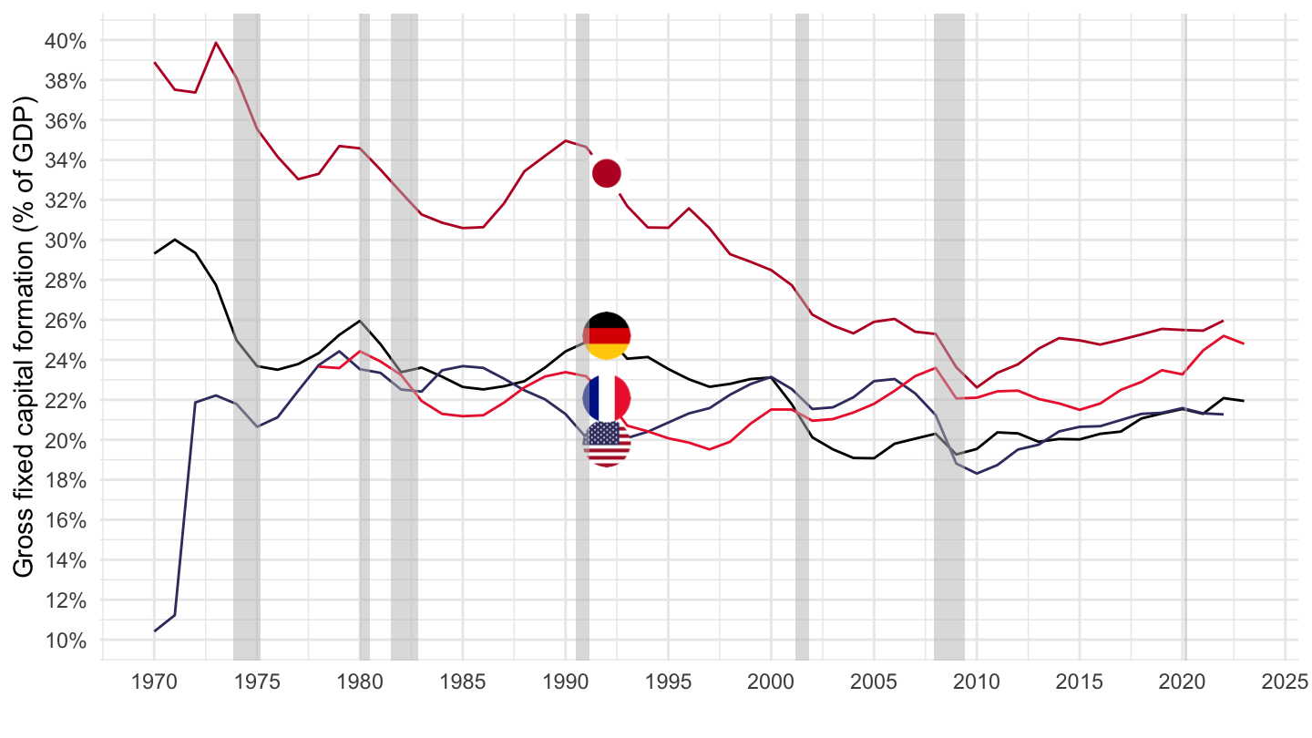
nber_recessions_extract <- nber_recessions |>
  filter(Peak >= as.Date("1970-01-01"))
NAAG |>
  filter(REF_AREA %in% c("FRA", "USA", "DEU", "JPN"),
         INDICATOR == "B9S1S") |>
  year_to_date() |>
  mutate(value = obsValue / 100) |>
  left_join(NAAG_var$LOCATION, by = c("REF_AREA" = "LOCATION")) |>
  add_flag_color("Location") |>
  ggplot() + geom_line(aes(x = date, y = obsValue / 100, color = color)) +
  scale_color_identity() + add_4flags +
  theme_minimal() + xlab("") + ylab("Net lending, Total economy, % of GDP") +
  geom_rect(data = nber_recessions_extract,
            aes(xmin = Peak, xmax = Trough, ymin = -Inf, ymax = +Inf),
            fill = 'grey', alpha = 0.5) +
  scale_x_date(breaks = seq(1960, 2100, 5) |> paste0("-01-01") |> as.Date(),
               labels = date_format("%Y")) +
  scale_y_continuous(breaks = 0.01*seq(-20, 50, 1),
                     labels = percent_format(accuracy = 1)) +
  theme(legend.position = c(0.2, 0.80),
        legend.title = element_blank())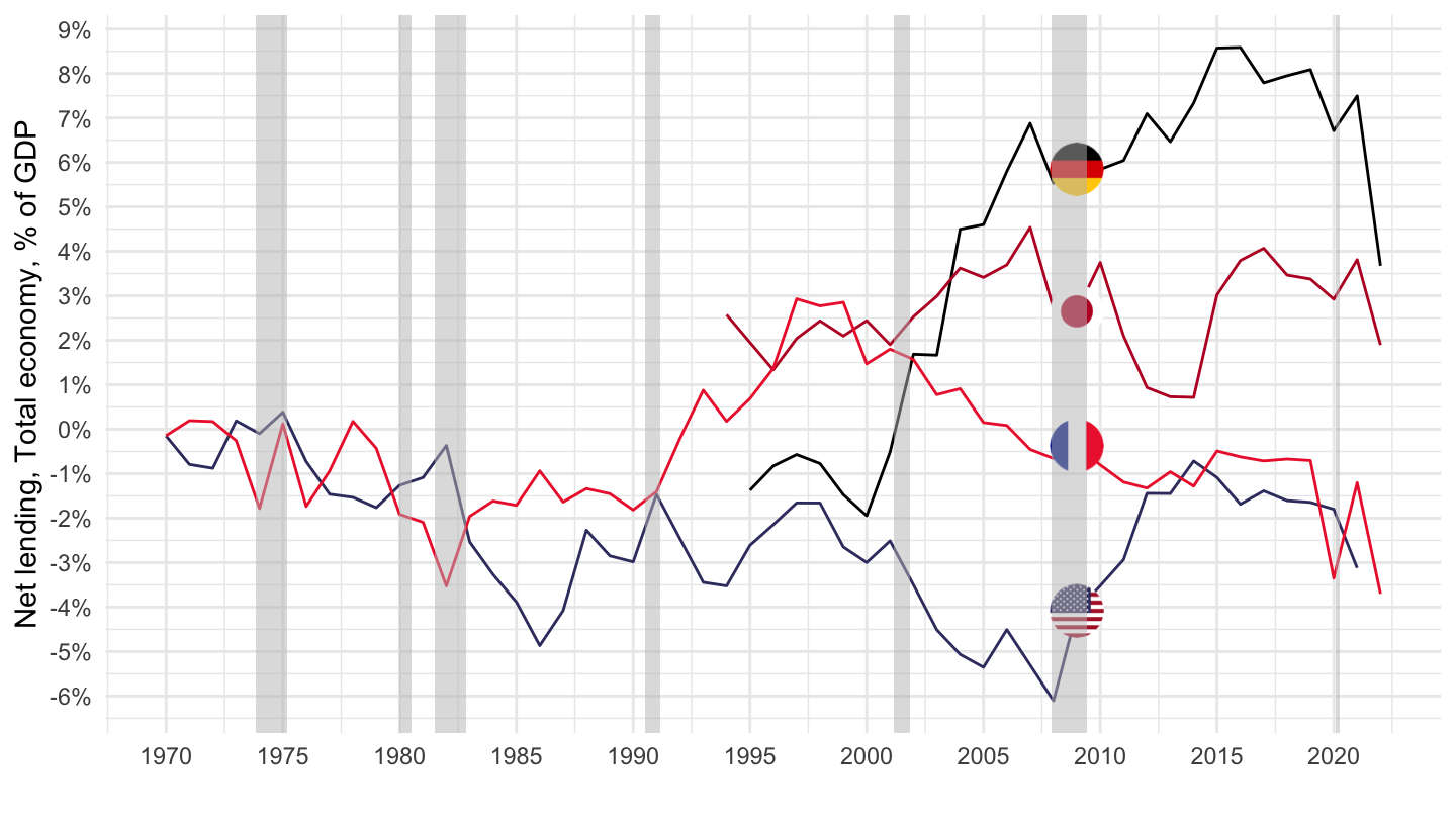
nber_recessions_extract <- nber_recessions |>
  filter(Peak >= as.Date("1970-01-01"))
NAAG |>
  filter(REF_AREA %in% c("FRA", "USA", "DEU", "JPN"),
         INDICATOR == "P51N11131SP51") |>
  year_to_date() |>
  mutate(value = obsValue / 100) |>
  left_join(NAAG_var$LOCATION, by = c("REF_AREA" = "LOCATION")) |>
  add_flag_color("Location") |>
  ggplot() + geom_line(aes(x = date, y = obsValue / 100, color = color)) +
  scale_color_identity() + add_4flags +
  theme_minimal() + xlab("") + ylab("Transport equipment, % of total GFCF") +
  geom_rect(data = nber_recessions_extract,
            aes(xmin = Peak, xmax = Trough, ymin = -Inf, ymax = +Inf),
            fill = 'grey', alpha = 0.5) +
  scale_x_date(breaks = seq(1960, 2100, 5) |> paste0("-01-01") |> as.Date(),
               labels = date_format("%Y")) +
  scale_y_continuous(breaks = 0.01*seq(0, 50, 1),
                     labels = percent_format(accuracy = 1))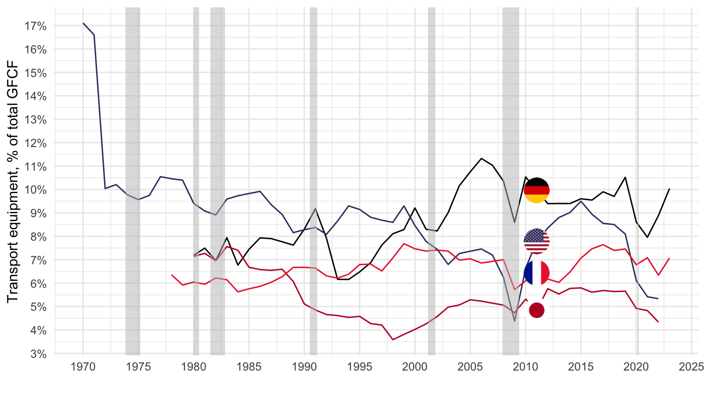
| source | dataset | Title | Updated |
|---|---|---|---|
| source | dataset | Title | Updated |
|---|---|---|---|
| source | dataset | Title | Updated |
|---|---|---|---|





