Quarterly Financial Accounts
Data - Banque de France
Info
Last observation: Trimestriel: 30 sep 2024 (N = 22,870) · Annuel: 31 déc 2023 (N = 1,479)
First observation: Trimestriel: 31 déc 1995 (N = 22,870) · Annuel: 31 déc 1995 (N = 1,479)
Last data update: 10 aoû 2026, 16:21. Last compile: 14 aoû 2026, 00:24
Structure
- Methodology. pdf
Last
| date | Nobs |
|---|---|
| 2024-09-30 | 4 |
List of publications
Info
Households’ financial saving and wealth, Financial accounts of non-financial agents, 15 April 2024, 2023Q4. pdf html
Households’ financial saving and wealth, 2023Q3. pdf
Households’ financial saving and wealth, 2023Q2. pdf
Quarterly presentation of household saving, 2023Q1. html pdf
Methodology. pdf
List of series. html
Households’ financial saving and wealth, 2022Q2. pdf
Household saving, 2021Q1. pdf
Debt ratio of non-financial agents – International comparisons, 2020Q4. html / pdf
Household saving, 2020Q3. pdf
INSTR_ASSET Instrument and assets classification
Code
CFT |>


  group_by(INSTR_ASSET, Instr_asset) |>
  summarise(Nobs = n()) |>
  #arrange(-Nobs) %>%
  print_table_conditional()
Main aggregates
2024Q2
Code
ig_b("bdf", "CFT-2024T2")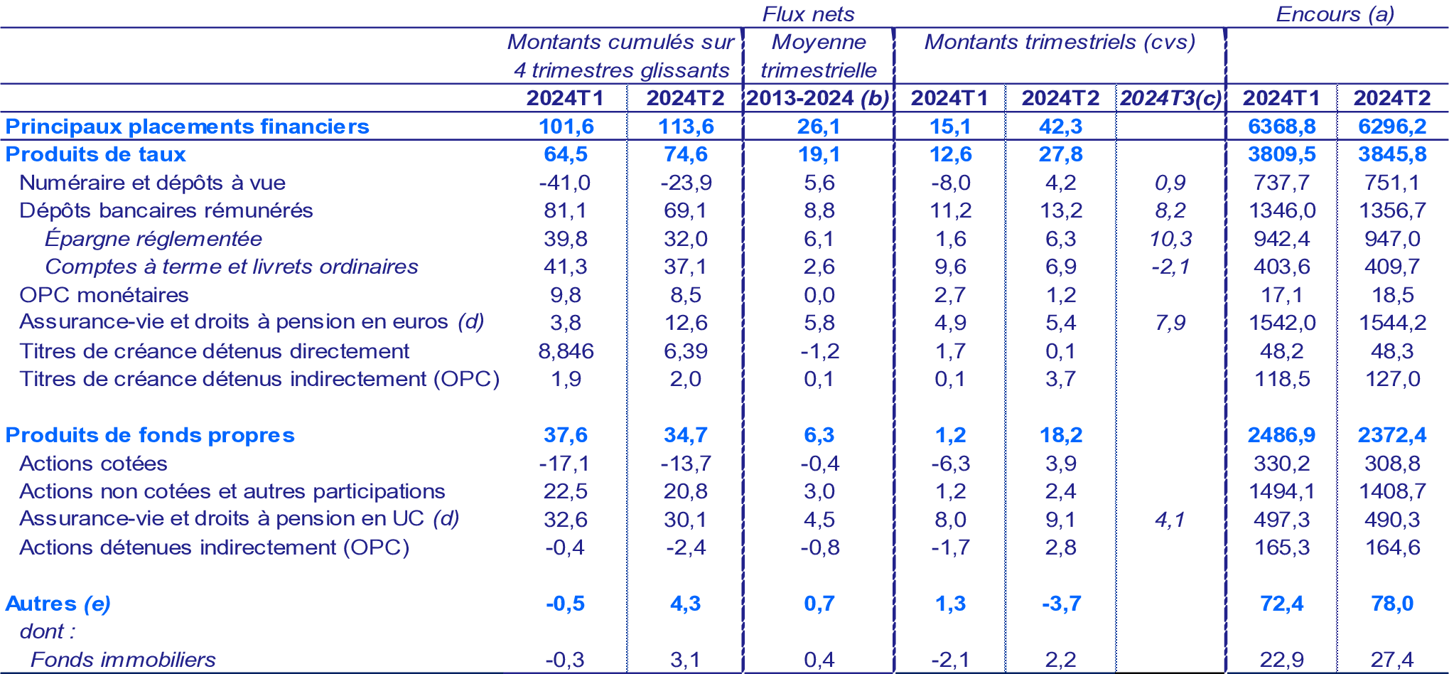
2023Q4
Code
ig_b("bdf", "CFT-2023T4")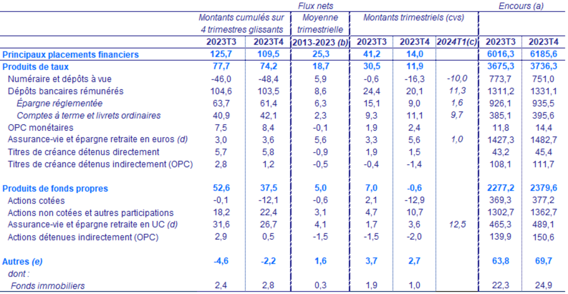
Fixed-income products
Code
CFT |>

  filter(STO == "LE",
         INSTR_ASSET %in% c("PDTX")) |>
  na.omit() |>
  ggplot() + geom_line(aes(x = date, y = value, color = Variable)) +
  xlab("") + ylab("") + theme_minimal() +
  scale_x_date(breaks = "1 year",
               labels = date_format("%Y")) +
  scale_y_log10(breaks = seq(-200, 10000, 100),
                     labels = dollar_format(acc = 1, prefix = "", su = "Mds€")) +
  theme(legend.position = c(0.35, 0.9),
        legend.title = element_blank(),
        legend.direction = "vertical") +
  geom_label(data = . %>% filter(date == as.Date("2023-12-31")),
             aes(x = date, y = value, color = Variable, label = round(value)))
Equity products
Code
CFT |>

  filter(STO == "LE",
         INSTR_ASSET %in% c("PDFP")) |>
  na.omit() |>
  ggplot() + geom_line(aes(x = date, y = value, color = Variable)) +
  xlab("") + ylab("") + theme_minimal() +
  scale_x_date(breaks = "1 year",
               labels = date_format("%Y")) +
  scale_y_log10(breaks = seq(-200, 10000, 100),
                     labels = dollar_format(acc = 1, prefix = "", su = "Mds€")) +
  theme(legend.position = c(0.35, 0.9),
        legend.title = element_blank(),
        legend.direction = "vertical") +
  geom_label(data = . %>% filter(date == as.Date("2023-12-31")),
             aes(x = date, y = value, color = Variable, label = round(value)))
Listed, unlisted
Code
CFT |>

  filter(STO == "LE",
         INSTR_ASSET %in% c("PDFP", "F51", "F511", "F51M", "F52")) |>
  na.omit() |>
  ggplot() + geom_line(aes(x = date, y = value, color = Variable)) +
  xlab("") + ylab("") + theme_minimal() +
  scale_x_date(breaks = "1 year",
               labels = date_format("%Y")) +
  scale_y_log10(breaks = seq(-200, 10000, 100),
                     labels = dollar_format(acc = 1, prefix = "", su = "Mds€")) +
  theme(legend.position = c(0.5, 0.7),
        legend.title = element_blank(),
        legend.direction = "vertical") +
  geom_label(data = . %>% filter(date == as.Date("2023-12-31")),
             aes(x = date, y = value, color = Variable, label = round(value)))
Detail
Linear
Code
CFT |>

  filter(STO == "LE",
         INSTR_ASSET %in% c("F62A", "F62B", "F29R", "F2A", "F29Z")) |>
  na.omit() |>
  ggplot() + geom_line(aes(x = date, y = value, color = Variable)) +
  xlab("") + ylab("") + theme_minimal() +
  scale_x_date(breaks = "1 year",
               labels = date_format("%Y")) +
  scale_y_continuous(breaks = seq(-200, 10000, 100),
                     labels = dollar_format(acc = 1, prefix = "", su = "Mds€")) +
  theme(legend.position = c(0.45, 0.17),
        legend.title = element_blank(),
        legend.direction = "vertical") +
  geom_label(data = . %>% filter(date == as.Date("2023-12-31")),
             aes(x = date, y = value, color = Variable, label = round(value)))
Log
Code
CFT |>

  filter(STO == "LE",
         INSTR_ASSET %in% c("F62A", "F62B", "F29R", "F2A", "F29Z")) |>
  na.omit() |>
  ggplot() + geom_line(aes(x = date, y = value, color = Variable)) +
  xlab("") + ylab("") + theme_minimal() +
  scale_x_date(breaks = "1 year",
               labels = date_format("%Y")) +
  scale_y_log10(breaks = seq(-200, 10000, 100),
                     labels = dollar_format(acc = 1, prefix = "", su = "Mds€")) +
  theme(legend.position = c(0.45, 0.17),
        legend.title = element_blank(),
        legend.direction = "vertical") +
  geom_label(data = . %>% filter(date == as.Date("2023-12-31")),
             aes(x = date, y = value, color = Variable, label = round(value)))
Outstanding amounts
Currency and overnight deposits
Code
CFT |>


  filter(REF_AREA %in% c("FR", "IT", "DE"),
         INSTR_ASSET == "F2A",
         STO == "LE") |>
  mutate(Ref_area = ifelse(REF_AREA == "I8", "Europe", Ref_area)) |>
  left_join(colors, by = c("Ref_area" = "country")) |>
  na.omit() |>
  ggplot() + geom_line(aes(x = date, y = value, color = color)) +
  xlab("") + ylab("") + theme_minimal() + scale_color_identity() + add_3flags +
  scale_x_date(breaks = "1 year",
               labels = date_format("%Y")) +
  scale_y_log10(breaks = seq(100, 4000, 100),
                labels = dollar_format(accuracy = 1, pre = "", su = " Mds€")) +
  geom_label(data = . %>% filter(date == as.Date("2023-12-31")),
             aes(x = date, y = value, label = round(value)))
Outstanding amounts
Code
CFT |>


  filter(REF_AREA %in% c("FR"),
         INSTR_ASSET %in% c("F2A", "F29Z", "F62B", "F29R"),
         STO == "LE") |>
  select(date, value, Instr_asset) |>
  na.omit() |>
  ggplot() + geom_line(aes(x = date, y = value, color = Instr_asset)) +
  xlab("") + ylab("") + theme_minimal() +

  scale_x_date(breaks = "1 year",
               labels = date_format("%Y")) +
  scale_y_log10(breaks = seq(100, 4000, 100),
                labels = dollar_format(accuracy = 1, pre = "", su = " Mds€")) +
  theme(legend.position = c(0.4, 0.4),
        legend.title = element_blank(),
        legend.direction = "vertical") +
  geom_label(data = . %>% filter(date == as.Date("2023-12-31")),
             aes(x = date, y = value, color = Instr_asset, label = round(value)))
Currency and overnight deposits
Outstanding amounts
All
Code
CFT |>


  filter(REF_AREA %in% c("FR"),
         INSTR_ASSET %in% c("F2A", "F29Z", "F62B"),
         STO == "LE") |>
  select(date, value, Instr_asset) |>
  na.omit() |>
  ggplot() + geom_line(aes(x = date, y = value, color = Instr_asset)) +
  xlab("") + ylab("") + theme_minimal() +

  scale_x_date(breaks = "1 year",
               labels = date_format("%Y")) +
  scale_y_log10(breaks = seq(100, 4000, 100),
                labels = dollar_format(accuracy = 1, pre = "", su = " Mds€")) +
  theme(legend.position = c(0.4, 0.4),
        legend.title = element_blank(),
        legend.direction = "vertical") +
  geom_label(data = . %>% filter(date == as.Date("2023-12-31")),
             aes(x = date, y = value, color = Instr_asset, label = round(value)))
2019-
Code
CFT |>


  filter(REF_AREA %in% c("FR"),
         INSTR_ASSET %in% c("F2A", "F29Z", "F62B"),
         STO == "LE") |>
  select(date, value, Instr_asset) |>
  na.omit() |>
  filter(date >= as.Date("2022-01-01")) |>
  ggplot() + geom_line(aes(x = date, y = value, color = Instr_asset)) +
  xlab("") + ylab("") + theme_minimal() +

  scale_x_date(breaks = "3 months",
               labels = date_format("%b %Y")) +
  scale_y_log10(breaks = seq(100, 4000, 100),
                labels = dollar_format(accuracy = 1, pre = "", su = " Mds€")) +
  theme(legend.position = c(0.4, 0.4),
        legend.title = element_blank(),
        legend.direction = "vertical") +
  geom_label(data = . %>% filter(date == as.Date("2023-12-31")),
             aes(x = date, y = value, color = Instr_asset, label = round(value)))
Flows - 4 quarters
Code
CFT |>


  filter(REF_AREA %in% c("FR"),
         INSTR_ASSET %in% c("F2A", "F29Z", "F62B", "F29R"),
         STO == "F",
         TRANSFORMATION == "C4") |>
  #filter(date >= as.Date("2016-01-01")) %>%
  select(date, value, Instr_asset) |>
  na.omit() |>
  ggplot() + geom_line(aes(x = date, y = value, color = Instr_asset)) +
  xlab("") + ylab("") + theme_minimal() +

  scale_x_date(breaks = "1 year",
               labels = date_format("%Y")) +
  scale_y_continuous(breaks = seq(-2000, 4000, 10),
                labels = dollar_format(accuracy = 1, pre = "", su = " Mds€")) +
  theme(legend.position = c(0.4, 0.8),
        legend.title = element_blank(),
        legend.direction = "vertical")
Flows
All
Code
CFT |>


  filter(REF_AREA %in% c("FR"),
         INSTR_ASSET %in% c("F2A", "F29Z", "F62B", "F29R"),
         STO == "F",
         TRANSFORMATION == "N",
         FREQ == "Q") |>
  filter(date >= as.Date("2010-01-01")) |>
  ggplot() + geom_line(aes(x = date, y = value, color = Instr_asset)) +
  xlab("") + ylab("") + theme_minimal() +

  scale_x_date(breaks = "1 year",
               labels = date_format("%Y")) +
  scale_y_continuous(breaks = seq(-1000, 4000, 10),
                labels = dollar_format(accuracy = 1, pre = "", su = " Mds€")) +
  theme(legend.position = c(0.4, 0.8),
        legend.title = element_blank(),
        legend.direction = "vertical")
2016
Code
CFT |>


  filter(REF_AREA %in% c("FR"),
         INSTR_ASSET %in% c("F2A", "F29Z", "F62B", "F29R"),
         STO == "F",
         TRANSFORMATION == "N",
         FREQ == "Q") |>
  filter(date >= as.Date("2016-01-01")) |>
  ggplot() + geom_line(aes(x = date, y = value, color = Instr_asset)) +
  xlab("") + ylab("") + theme_minimal() +

  scale_x_date(breaks = "1 year",
               labels = date_format("%Y")) +
  scale_y_continuous(breaks = seq(-1000, 4000, 10),
                labels = dollar_format(accuracy = 1, pre = "", su = " Mds€")) +
  theme(legend.position = c(0.4, 0.9),
        legend.title = element_blank(),
        legend.direction = "vertical") +
  geom_hline(yintercept = 0, linetype = "dashed")
Listed/unlisted shares, unit-linked life insurance
Outstanding amounts
Code
CFT |>


  filter(REF_AREA %in% c("FR"),
         INSTR_ASSET %in% c( "F511", "F51M", "F51"),
         STO == "LE") |>
  na.omit() |>
  ggplot() + geom_line(aes(x = date, y = value, color = Instr_asset)) +
  xlab("") + ylab("") + theme_minimal() +

  scale_x_date(breaks = "1 year",
               labels = date_format("%Y")) +
  scale_y_log10(breaks = seq(100, 4000, 100),
                labels = dollar_format(accuracy = 1, pre = "", su = " Mds€")) +
  theme(legend.position = c(0.4, 0.6),
        legend.title = element_blank(),
        legend.direction = "vertical") +
  geom_label(data = . %>% filter(date == as.Date("2023-12-31")),
             aes(x = date, y = value, color = Instr_asset, label = round(value)))
Listed/unlisted shares, unit-linked life insurance
Outstanding amounts
Code
CFT |>


  filter(REF_AREA %in% c("FR"),
         INSTR_ASSET %in% c( "F511", "F51M", "F62A"),
         STO == "LE") |>
  na.omit() |>
  ggplot() + geom_line(aes(x = date, y = value, color = Instr_asset)) +
  xlab("") + ylab("") + theme_minimal() +

  scale_x_date(breaks = "1 year",
               labels = date_format("%Y")) +
  scale_y_log10(breaks = seq(100, 4000, 100),
                labels = dollar_format(accuracy = 1, pre = "", su = " Mds€")) +
  theme(legend.position = c(0.4, 0.6),
        legend.title = element_blank(),
        legend.direction = "vertical") +
  geom_label(data = . %>% filter(date == as.Date("2023-12-31")),
             aes(x = date, y = value, color = Instr_asset, label = round(value)))
Flows
Code
CFT |>


  filter(REF_AREA %in% c("FR"),
         INSTR_ASSET %in% c( "F511", "F51M", "F62A"),
         STO == "F",
         TRANSFORMATION == "N",
         FREQ == "Q") |>
  filter(date >= as.Date("2016-01-01")) |>
  ggplot() + geom_line(aes(x = date, y = value, color = Instr_asset)) +
  xlab("") + ylab("") + theme_minimal() +

  scale_x_date(breaks = "1 year",
               labels = date_format("%Y")) +
  scale_y_continuous(breaks = seq(-2000, 4000, 5),
                labels = dollar_format(accuracy = 1, pre = "", su = " Mds€")) +
  theme(legend.position = c(0.4, 0.4),
        legend.title = element_blank(),
        legend.direction = "vertical")
Currency and overnight deposits
Code
CFT |>


  filter(REF_AREA %in% c("FR"),
         INSTR_ASSET %in% c("F2A", "F29Z"),
         STO == "LE") |>
  na.omit() |>
  ggplot() + geom_line(aes(x = date, y = value, color = Instr_asset)) +
  xlab("") + ylab("") + theme_minimal() +

  scale_x_date(breaks = "1 year",
               labels = date_format("%Y")) +
  scale_y_log10(breaks = seq(100, 4000, 100),
                labels = dollar_format(accuracy = 1, pre = "", su = " Mds€")) +
  theme(legend.position = c(0.75, 0.1),
        legend.title = element_blank(),
        legend.direction = "vertical") +
  geom_label(data = . %>% filter(date == as.Date("2023-12-31")),
             aes(x = date, y = value, color = Instr_asset, label = round(value)))
Life insurance
All
2007-
Code
CFT |>

  filter(variable %in% c("CFT.Q.S.FR.W0.S1M.S1.N.A.F.F62B._Z._Z.XDC._T.S.V.N._T",
                         "CFT.Q.S.FR.W0.S1M.S1.N.A.F.F62A._Z._Z.XDC._T.S.V.N._T",
                         "CFT.Q.S.FR.W0.S1M.S1.N.A.F.F29R.T._Z.XDC._T.S.V.N._T",
                         "CFT.Q.S.FR.W0.S1M.S1.N.A.F.F2A.T._Z.XDC._T.S.V.N._T")) |>
  na.omit() |>
  ggplot() + geom_line(aes(x = date, y = value, color = Variable)) +
  xlab("") + ylab("") + theme_minimal() +

  scale_x_date(breaks = "1 year",
               labels = date_format("%Y")) +
  scale_y_continuous(breaks = seq(-200, 1000, 5),
                     limits = c(-25 ,40),
                     labels = dollar_format(acc = 1, prefix = "", su = "Mds€")) +
  theme(legend.position = c(0.45, 0.17),
        legend.title = element_blank(),
        legend.direction = "vertical")
2015-
Code
CFT |>

  filter(variable %in% c("CFT.Q.S.FR.W0.S1M.S1.N.A.F.F62B._Z._Z.XDC._T.S.V.N._T",
                         "CFT.Q.S.FR.W0.S1M.S1.N.A.F.F29Z.T._Z.XDC._T.S.V.N._T",
                         "CFT.Q.S.FR.W0.S1M.S1.N.A.F.F29R.T._Z.XDC._T.S.V.N._T",
                         "CFT.Q.S.FR.W0.S1M.S1.N.A.F.F2A.T._Z.XDC._T.S.V.N._T")) |>
  filter(date >= as.Date("2015-01-01")) |>
  ggplot() + geom_line(aes(x = date, y = value, color = Variable)) +
  xlab("") + ylab("") + theme_minimal() +

  scale_x_date(breaks = "1 year",
               labels = date_format("%Y")) +
  scale_y_continuous(breaks = seq(-200, 1000, 5),
                     limits = c(-5 ,40),
                     labels = dollar_format(acc = 1, prefix = "", su = "Mds€")) +
  theme(legend.position = c(0.45, 0.8),
        legend.title = element_blank(),
        legend.direction = "vertical")
Household saving rate
The household saving rate is the ratio of households’ gross saving (B8G) to gross disposable income adjusted for changes in pension entitlements. Gross disposable income (B6G) corresponds to the income received by households (earned income and property income) after redistribution operations (adding cash social benefits received, subtracting contributions and taxes).
As for the financial saving rate, it is the share of gross disposable income invested in financial assets.
the saving rate is obtained by dividing gross saving by gross disposable income adjusted for the change in households’ entitlements under pension funds, with both series previously seasonally adjusted
the financial saving rate is estimated by subtracting gross fixed capital formation from gross saving, then dividing the result by gross disposable income adjusted for the change in households’ entitlements under pension funds, and then seasonally adjusting the result.
Annual
Code
CFT |>

  filter(variable %in% c("CFT.A.N.FR.W0.S1M.S1.N.B.B8G._Z._Z._Z.XDC_R_B6G_S1M._T.S.V.N._T",
                         "CFT.A.N.FR.W0.S1M.S1.N.B.B9Z._Z._Z._Z.XDC_R_B6G_S1M._T.S.V.N._T")) |>
  na.omit() |>
  ggplot() + geom_line(aes(x = date, y = value/100, color = Variable)) +
  xlab("") + ylab("") + theme_minimal() +

  scale_x_date(breaks = "1 year",
               labels = date_format("%Y")) +
  scale_y_continuous(breaks = 0.01*seq(-10, 100, 1),
                labels = percent_format(accuracy = 1)) +
  theme(legend.position = c(0.4, 0.9),
        legend.title = element_blank(),
        legend.direction = "vertical")
Quarterly
All
Code
CFT |>

  filter(variable %in% c("CFT.Q.N.FR.W0.S1M.S1.N.B.B8G._Z._Z._Z.XDC_R_B6G_S1M._T.S.V.C4._T",
                         "CFT.Q.N.FR.W0.S1M.S1.N.B.B9Z._Z._Z._Z.XDC_R_B6G_S1M._T.S.V.C4._T")) |>
  na.omit() |>
  ggplot() + geom_line(aes(x = date, y = value/100, color = Variable)) +
  xlab("") + ylab("") + theme_minimal() +
  scale_x_date(breaks = "2 years",
               labels = date_format("%Y")) +
  scale_y_continuous(breaks = 0.01*seq(-10, 100, 1),
                labels = percent_format(accuracy = 1)) +
  theme(legend.position = c(0.42, 0.9),
        legend.title = element_blank(),
        legend.direction = "vertical")
2010-
Code
CFT |>

  filter(variable %in% c("CFT.Q.N.FR.W0.S1M.S1.N.B.B8G._Z._Z._Z.XDC_R_B6G_S1M._T.S.V.C4._T",
                         "CFT.Q.N.FR.W0.S1M.S1.N.B.B9Z._Z._Z._Z.XDC_R_B6G_S1M._T.S.V.C4._T")) |>
  na.omit() |>
  filter(date >= as.Date("2010-01-01")) |>
  ggplot() + geom_line(aes(x = date, y = value/100, color = Variable)) +
  xlab("") + ylab("") + theme_minimal() +
  scale_x_date(breaks = "2 years",
               labels = date_format("%Y")) +
  scale_y_continuous(breaks = 0.01*seq(-10, 100, 1),
                labels = percent_format(accuracy = 1)) +
  theme(legend.position = c(0.45, 0.9),
        legend.title = element_blank(),
        legend.direction = "vertical")
France, Spain, Italy
Table
Code
REF_AREA <- read_parquet("REF_AREA.parquet")
CFT |>


  filter(FREQ == "Q",
         UNIT_MEASURE == "XDC_R_B6G_S1M",
         REF_SECTOR == "S1M",
         date == as.Date("2020-01-01")) |>
  select(Variable, Ref_area, value) |>
  arrange(Ref_area) |>
print_table_conditional()| Variable | Ref_area | value |
|---|---|---|
| NA | NA | NA |
| :--------: | :--------: | :-----: |
Financial saving rate
France, Italy, Germany
Code
CFT |>


  filter(FREQ == "Q",
         REF_AREA %in% c("FR", "IT", "DE"),
         UNIT_MEASURE == "XDC_R_B6G_S1M",
         STO == "B9Z",
         REF_SECTOR == "S1M") |>
  mutate(value = value/100) |>
  na.omit() |>
  ggplot() + geom_line(aes(x = date, y = value, color = Ref_area)) +
  xlab("") + ylab("") + theme_minimal() +
  scale_color_manual(values = c("#002395", "#000000", "#009246")) +
  scale_x_date(breaks = "2 years",
               labels = date_format("%Y")) +
  add_3flags +
  scale_y_continuous(breaks = 0.01*seq(-10, 100, 1),
                labels = percent_format(accuracy = 1)) +
  theme(legend.position = "none")
France, Italy, Germany, Spain, United States
All
Code
CFT |>


  filter(FREQ == "Q",
         UNIT_MEASURE == "XDC_R_B6G_S1M",
         STO == "B9Z",
         REF_SECTOR == "S1M") |>
  left_join(colors, by = c("Ref_area" = "country")) |>
  mutate(value = value/100) |>
  na.omit() |>
  ggplot() + geom_line(aes(x = date, y = value, color = color)) +
  xlab("") + ylab("") + theme_minimal() + scale_color_identity() + add_6flags +
  scale_x_date(breaks = "2 years",
               labels = date_format("%Y")) +
  scale_y_continuous(breaks = 0.01*seq(-10, 100, 1),
                labels = percent_format(accuracy = 1))
2007-
Code
CFT |>


  filter(FREQ == "Q",
         UNIT_MEASURE == "XDC_R_B6G_S1M",
         STO == "B9Z",
         REF_SECTOR == "S1M") |>
  left_join(colors, by = c("Ref_area" = "country")) |>
  mutate(value = value/100) |>
  filter(date >= as.Date("2007-01-01")) |>
  na.omit() |>
  ggplot() + geom_line(aes(x = date, y = value, color = color)) +
  xlab("") + ylab("") + theme_minimal() + scale_color_identity() + add_6flags +
  scale_x_date(breaks = "1 year",
               labels = date_format("%Y")) +
  scale_y_continuous(breaks = 0.01*seq(-10, 100, 1),
                labels = percent_format(accuracy = 1))
2015-
Code
CFT |>


  filter(FREQ == "Q",
         UNIT_MEASURE == "XDC_R_B6G_S1M",
         STO == "B9Z",
         REF_SECTOR == "S1M") |>
  left_join(colors, by = c("Ref_area" = "country")) |>
  mutate(value = value/100) |>
  filter(date >= as.Date("2015-01-01")) |>
  na.omit() |>
  ggplot() + geom_line(aes(x = date, y = value, color = color)) +
  xlab("") + ylab("Financial saving rate (%)") + theme_minimal() + scale_color_identity() + add_6flags +
  scale_x_date(breaks = "1 year",
               labels = date_format("%Y")) +
  scale_y_continuous(breaks = 0.01*seq(-10, 100, 1),
                labels = percent_format(accuracy = 1))
Saving rate
France, Italy, Germany
Code
CFT |>


  filter(FREQ == "Q",
         REF_AREA %in% c("FR", "IT", "DE"),
         UNIT_MEASURE == "XDC_R_B6G_S1M",
         STO == "B8G",
         REF_SECTOR == "S1M") |>
  left_join(colors, by = c("Ref_area" = "country")) |>
  mutate(value = value/100) |>
  na.omit() |>
  ggplot() + geom_line(aes(x = date, y = value, color = color)) +
  xlab("") + ylab("") + theme_minimal() + scale_color_identity() + add_3flags +
  scale_x_date(breaks = "2 years",
               labels = date_format("%Y")) +
  scale_y_continuous(breaks = 0.01*seq(-10, 100, 1),
                labels = percent_format(accuracy = 1))
France, Italy, Germany, Spain, United States
Code
CFT |>


  filter(FREQ == "Q",
         UNIT_MEASURE == "XDC_R_B6G_S1M",
         STO == "B8G",
         REF_SECTOR == "S1M") |>
  left_join(colors, by = c("Ref_area" = "country")) |>
  mutate(value = value/100) |>
  na.omit() |>
  ggplot() + geom_line(aes(x = date, y = value, color = color)) +
  xlab("") + ylab("") + theme_minimal() + scale_color_identity() + add_6flags +
  scale_x_date(breaks = "2 years",
               labels = date_format("%Y")) +
  scale_y_continuous(breaks = 0.01*seq(-10, 100, 1),
                labels = percent_format(accuracy = 1))
Debt
Household debt
All
Code
CFT |>


  filter(INSTR_ASSET == "DETT",
         UNIT_MEASURE == "XDC_R_B1GQ_CY",
         REF_SECTOR == "S1M") |>
  mutate(Ref_area = ifelse(REF_AREA == "I8", "Europe", Ref_area)) |>
  mutate(Ref_area = ifelse(REF_AREA == "UK", "United Kingdom", Ref_area)) |>
  left_join(colors, by = c("Ref_area" = "country")) |>
  mutate(value = value/100) |>
  arrange(date) |>
  select(REF_AREA,everything()) |>
  ggplot() + geom_line(aes(x = date, y = value, color = color)) +
  xlab("") + ylab("") + theme_minimal() + scale_color_identity() + add_7flags +
  scale_x_date(breaks = "2 years",
               labels = date_format("%Y")) +
  scale_y_continuous(breaks = 0.01*seq(-10, 200, 10),
                labels = percent_format(accuracy = 1))
France, Italy, Germany, Spain, Japan, EU
Code
CFT |>


  filter(REF_AREA %in% c("FR", "IT", "DE", "ES", "JP", "I8"),
         INSTR_ASSET == "DETT",
         UNIT_MEASURE == "XDC_R_B1GQ_CY",
         REF_SECTOR == "S1M") |>
  mutate(Ref_area = ifelse(REF_AREA == "I8", "Europe", Ref_area)) |>
  left_join(colors, by = c("Ref_area" = "country")) |>
  mutate(value = value/100) |>
  ggplot() + geom_line(aes(x = date, y = value, color = color)) +
  xlab("") + ylab("") + theme_minimal() + scale_color_identity() + add_6flags +
  scale_x_date(breaks = "2 years",
               labels = date_format("%Y")) +
  scale_y_continuous(breaks = 0.01*seq(-10, 100, 5),
                labels = percent_format(accuracy = 1))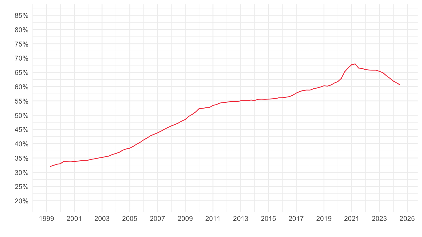
France, Italy, Germany
All
Code
CFT |>


  filter(REF_AREA %in% c("FR", "IT", "DE"),
         INSTR_ASSET == "DETT",
         UNIT_MEASURE == "XDC_R_B1GQ_CY",
         REF_SECTOR == "S1M") |>
  mutate(Ref_area = ifelse(REF_AREA == "I8", "Europe", Ref_area)) |>
  left_join(colors, by = c("Ref_area" = "country")) |>
  mutate(value = value/100) |>
  ggplot() + geom_line(aes(x = date, y = value, color = color)) +
  xlab("") + ylab("") + theme_minimal() + scale_color_identity() + add_3flags +
  scale_x_date(breaks = "2 years",
               labels = date_format("%Y")) +
  scale_y_continuous(breaks = 0.01*seq(-10, 100, 5),
                labels = percent_format(accuracy = 1))
2013-
Code
CFT |>


  filter(REF_AREA %in% c("FR", "IT", "DE"),
         INSTR_ASSET == "DETT",
         UNIT_MEASURE == "XDC_R_B1GQ_CY",
         REF_SECTOR == "S1M") |>
  mutate(Ref_area = ifelse(REF_AREA == "I8", "Europe", Ref_area)) |>
  left_join(colors, by = c("Ref_area" = "country")) |>
  mutate(value = value/100) |>
  filter(date >=as.Date("2013-01-01")) |>
  ggplot() + geom_line(aes(x = date, y = value, color = color)) +
  xlab("") + ylab("") + theme_minimal() + scale_color_identity() + add_3flags +
  scale_x_date(breaks = "1 year",
               labels = date_format("%Y")) +
  scale_y_continuous(breaks = 0.01*seq(-10, 100, 2),
                labels = percent_format(accuracy = 1))
Non-financial corporations
France, Italy, Germany
Code
CFT |>


  filter(REF_AREA %in% c("FR", "IT", "DE", "I8"),
         INSTR_ASSET == "DETT",
         UNIT_MEASURE == "XDC_R_B1GQ_CY",
         REF_SECTOR == "S11") |>
  mutate(Ref_area = ifelse(REF_AREA == "I8", "Europe", Ref_area)) |>
  left_join(colors, by = c("Ref_area" = "country")) |>
  mutate(value = value/100) |>
  ggplot() + geom_line(aes(x = date, y = value, color = color)) +
  xlab("") + ylab("") + theme_minimal() + scale_color_identity() + add_4flags +
  scale_x_date(breaks = "2 years",
               labels = date_format("%Y")) +
  scale_y_continuous(breaks = 0.01*seq(-10, 100, 5),
                labels = dollar_format(accuracy = .01, pre = "", su = " année"))
Debt ratio
France
Years of GDP
Code
CFT |>

  filter(variable %in% c("CFT.Q.S.FR.W0.S1M.S1.N.L.LE.DETT.T._Z.XDC_R_B1GQ_CY._T.S.V.N._T",
                         "CFT.Q.S.FR.W0.S11.S1.C.L.LE.DETT.T._Z.XDC_R_B1GQ_CY._T.S.V.N._T",
                         "CFT.Q.N.FR.W0.S13.S1.C.L.LE.GD.T._Z.XDC_R_B1GQ_CY._T.F.V.N._T")) |>
  mutate(Variable = gsub(", en % du PIB", "", Variable),
         Variable = gsub(" en % du PIB", "", Variable)) |>
  ggplot() + geom_line(aes(x = date, y = value/100, color = Variable)) +
  xlab("") + ylab("Debt/GDP (in years of GDP)") + theme_minimal() +

  scale_x_date(breaks = "2 years",
               labels = date_format("%Y")) +
  scale_y_continuous(breaks = seq(0, 1.3, 0.1),
                     labels = dollar_format(su = " ans", p = "", acc = 0.1)) +
  theme(legend.position = c(0.3, 0.9),
        legend.title = element_blank(),
        legend.direction = "vertical")
% of GDP
Code
CFT |>

  filter(variable %in% c("CFT.Q.S.FR.W0.S1M.S1.N.L.LE.DETT.T._Z.XDC_R_B1GQ_CY._T.S.V.N._T",
                         "CFT.Q.S.FR.W0.S11.S1.C.L.LE.DETT.T._Z.XDC_R_B1GQ_CY._T.S.V.N._T",
                         "CFT.Q.N.FR.W0.S13.S1.C.L.LE.GD.T._Z.XDC_R_B1GQ_CY._T.F.V.N._T")) |>
  ggplot() + geom_line(aes(x = date, y = value/100, color = Variable)) +
  xlab("") + ylab("") + theme_minimal() +

  scale_x_date(breaks = "2 years",
               labels = date_format("%Y")) +
  scale_y_continuous(breaks = 0.01*seq(-10, 140, 5),
                labels = percent_format(accuracy = 1)) +
  theme(legend.position = c(0.3, 0.9),
        legend.title = element_blank(),
        legend.direction = "vertical")
Germany
Code
CFT |>

  filter(variable %in% c("CFT.Q.N.DE.W0.S1M.S1.N.L.LE.DETT.T._Z.XDC_R_B1GQ_CY._T.S.V.N._T",
                         "CFT.Q.N.DE.W0.S11.S1.C.L.LE.DETT.T._Z.XDC_R_B1GQ_CY._T.S.V.N._T",
                         "CFT.Q.N.DE.W0.S13.S1.C.L.LE.GD.T._Z.XDC_R_B1GQ_CY._T.F.V.N._T")) |>
  ggplot() + geom_line(aes(x = date, y = value/100, color = Variable)) +
  xlab("") + ylab("") + theme_minimal() +

  scale_x_date(breaks = "2 years",
               labels = date_format("%Y")) +
  scale_y_continuous(breaks = 0.01*seq(-10, 140, 5),
                labels = percent_format(accuracy = 1)) +
  theme(legend.position = c(0.3, 0.9),
        legend.title = element_blank(),
        legend.direction = "vertical")
Italy
Code
CFT |>

  filter(variable %in% c("CFT.Q.N.IT.W0.S1M.S1.N.L.LE.DETT.T._Z.XDC_R_B1GQ_CY._T.S.V.N._T",
                         "CFT.Q.N.IT.W0.S11.S1.C.L.LE.DETT.T._Z.XDC_R_B1GQ_CY._T.S.V.N._T",
                         "CFT.Q.N.IT.W0.S13.S1.C.L.LE.GD.T._Z.XDC_R_B1GQ_CY._T.F.V.N._T")) |>
  ggplot() + geom_line(aes(x = date, y = value/100, color = Variable)) +
  xlab("") + ylab("") + theme_minimal() +

  scale_x_date(breaks = "2 years",
               labels = date_format("%Y")) +
  scale_y_continuous(breaks = 0.01*seq(-10, 400, 10),
                labels = percent_format(accuracy = 1)) +
  theme(legend.position = c(0.3, 0.9),
        legend.title = element_blank(),
        legend.direction = "vertical")
Spain
Code
CFT |>

  filter(variable %in% c("CFT.Q.N.ES.W0.S1M.S1.N.L.LE.DETT.T._Z.XDC_R_B1GQ_CY._T.S.V.N._T",
                         "CFT.Q.N.ES.W0.S11.S1.C.L.LE.DETT.T._Z.XDC_R_B1GQ_CY._T.S.V.N._T",
                         "CFT.Q.N.ES.W0.S13.S1.C.L.LE.GD.T._Z.XDC_R_B1GQ_CY._T.F.V.N._T")) |>
  ggplot() + geom_line(aes(x = date, y = value/100, color = Variable)) +
  xlab("") + ylab("") + theme_minimal() +

  scale_x_date(breaks = "2 years",
               labels = date_format("%Y")) +
  scale_y_continuous(breaks = 0.01*seq(-10, 400, 10),
                labels = percent_format(accuracy = 1)) +
  theme(legend.position = c(0.2, 0.9),
        legend.title = element_blank(),
        legend.direction = "vertical")
Euro area
Code
CFT |>

  filter(variable %in% c("CFT.Q.N.I8.W0.S1M.S1.N.L.LE.DETT.T._Z.XDC_R_B1GQ_CY._T.S.V.N._T",
                         "CFT.Q.N.I8.W0.S11.S1.C.L.LE.DETT.T._Z.XDC_R_B1GQ_CY._T.S.V.N._T",
                         "CFT.Q.N.I8.W0.S13.S1.C.L.LE.GD.T._Z.XDC_R_B1GQ_CY._T.F.V.N._T")) |>
  ggplot() + geom_line(aes(x = date, y = value/100, color = Variable)) +
  xlab("") + ylab("") + theme_minimal() +

  scale_x_date(breaks = "2 years",
               labels = date_format("%Y")) +
  scale_y_continuous(breaks = 0.01*seq(-10, 140, 5),
                labels = percent_format(accuracy = 1)) +
  theme(legend.position = c(0.3, 0.9),
        legend.title = element_blank(),
        legend.direction = "vertical")
Additional information
Data on the French macroeconomy
| source | dataset | Title | .html | .rData |
|---|---|---|---|---|
| bdf | CFT | Comptes Financiers Trimestriels | 2026-08-12 | 2026-08-10 |
| insee | CNA-2014-CONSO-SI | Dépenses de consommation finale par secteur institutionnel | 2026-08-13 | 2026-08-12 |
| insee | CNA-2014-CSI | Comptes des secteurs institutionnels | 2026-08-13 | 2026-08-12 |
| insee | CNA-2014-FBCF-BRANCHE | Formation brute de capital fixe (FBCF) par branche | 2026-08-13 | 2026-08-12 |
| insee | CNA-2014-FBCF-SI | Formation brute de capital fixe (FBCF) par secteur institutionnel | 2026-08-13 | 2026-08-12 |
| insee | CNA-2014-RDB | Revenu et pouvoir d’achat des ménages | 2026-08-13 | 2026-08-12 |
| insee | CNA-2020-CONSO-MEN | Consommation des ménages | 2026-08-13 | 2026-07-23 |
| insee | CNA-2020-PIB | Produit intérieur brut (PIB) et ses composantes | 2026-08-13 | 2026-08-12 |
| insee | CNT-2014-CB | Comptes des branches | 2026-08-13 | 2026-08-12 |
| insee | CNT-2014-CSI | Comptes de secteurs institutionnels | 2026-08-13 | 2026-08-12 |
| insee | CNT-2014-OPERATIONS | Opérations sur biens et services | 2026-08-13 | 2026-08-12 |
| insee | CNT-2014-PIB-EQB-RF | Équilibre du produit intérieur brut | 2026-08-13 | 2026-08-12 |
| insee | CONSO-MENAGES-2020 | Consommation des ménages en biens | 2026-08-13 | 2026-08-12 |
| insee | ICA-2015-IND-CONS | Indices de chiffre d'affaires dans l'industrie et la construction | 2026-08-13 | 2026-08-13 |
| insee | conso-mensuelle | Consommation de biens, données mensuelles | 2026-08-13 | 2026-08-02 |
| insee | t_1101 | 1.101 – Le produit intérieur brut et ses composantes à prix courants (En milliards d'euros) | 2026-08-13 | 2026-08-02 |
| insee | t_1102 | 1.102 – Le produit intérieur brut et ses composantes en volume aux prix de l'année précédente chaînés (En milliards d'euros 2014) | 2026-08-13 | 2026-08-02 |
| insee | t_1105 | 1.105 – Produit intérieur brut - les trois approches à prix courants (En milliards d'euros) - t_1105 | 2026-08-13 | 2026-08-02 |
Data on saving
| source | dataset | Title | .html | .rData |
|---|---|---|---|---|
| bdf | CFT | Comptes Financiers Trimestriels | 2026-08-12 | 2026-08-10 |
| bea | T50100 | Table 5.1. Saving and Investment by Sector (A) (Q) | 2026-08-12 | 2026-08-12 |
| fred | saving | Saving - saving | 2026-08-12 | 2026-08-12 |
| oecd | NAAG | National Accounts at a Glance - NAAG | 2026-08-13 | 2026-08-02 |
| wdi | NY.GDS.TOTL.ZS | Gross domestic savings (% of GDP) - NY.GDS.TOTL.ZS | 2026-08-12 | 2026-08-12 |
| wdi | NY.GNS.ICTR.ZS | Gross savings (% of GDP) - NY.GNS.ICTR.ZS | 2026-08-12 | 2026-08-12 |