
Last observation: Q2 2026 (N = 1730) · déc. 2018 (N = 95)
First observation: janv. 1991 (N = 1) · Q1 1991 (N = 1)
Last data update: 16 oct. 2026, 00:27
Last compile: 16 oct. 2026, 01:33
i_g("bib/dares/DI-2021T3/tab1.png")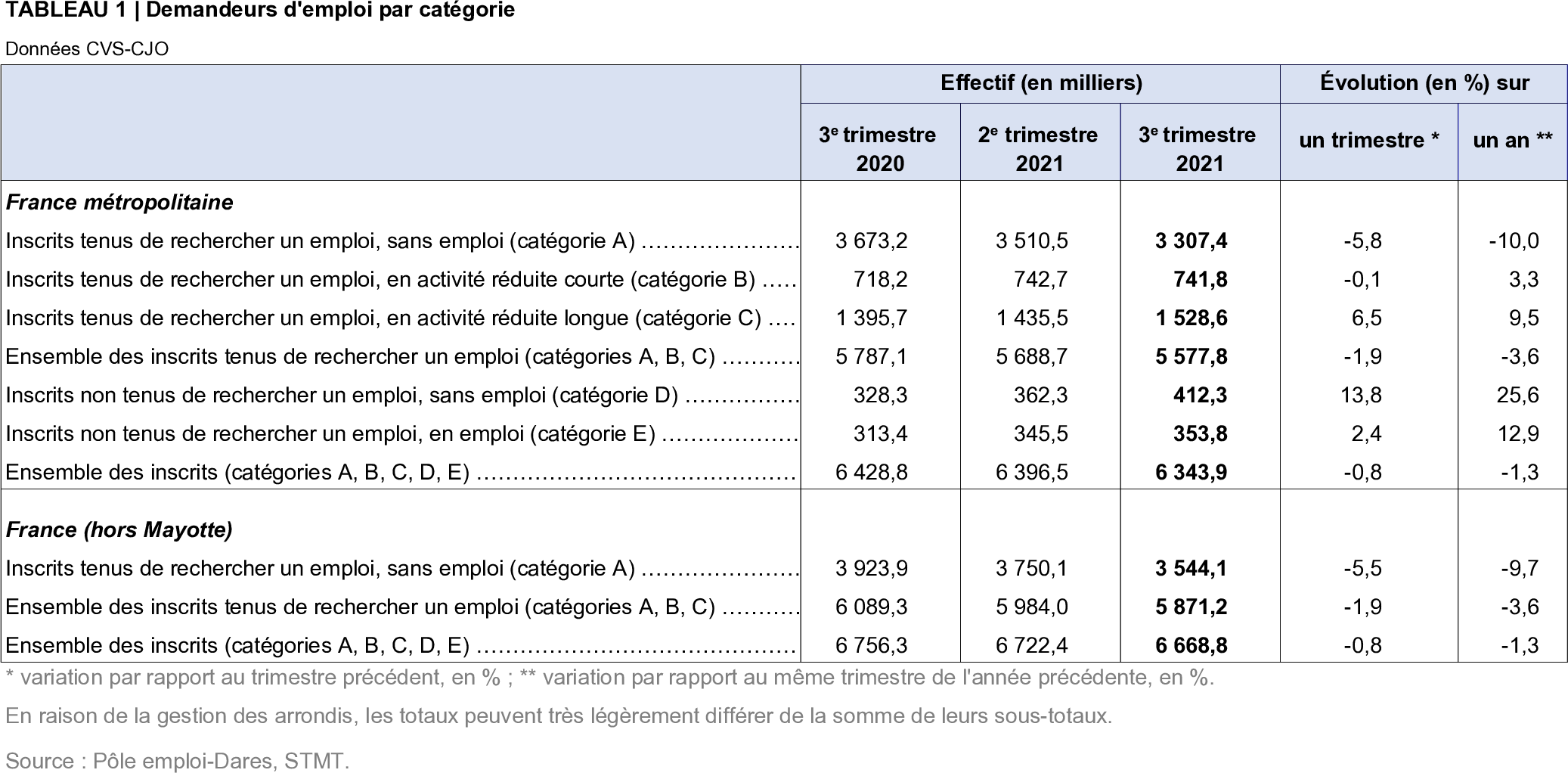
`DEMANDES-EMPLOIS-NATIONALES` |>
  filter(DEMANDEURS_EMPLOI == "A-B-C",
         INDICATEUR == "DEMANDEURS_EMPLOI_PE",
         METIER == "SO",
         SEXE == "0",
         FREQ == "T",
         CORRECTION == "CVS-CJO",
         ANCIENNETE == "SO",
         DIPLOME == "SO",
         AGE == "00-") |>
  quarter_to_date() |>
  arrange(date) |>
  mutate(OBS_VALUE = OBS_VALUE |> as.numeric()) |>
  ggplot() + theme_minimal() + xlab("") + ylab("Demandeurs emplois") +
  geom_line(aes(x = date, y = OBS_VALUE, color = REF_AREA)) +
  scale_x_date(breaks = seq(1960, 2100, 2) |> paste0("-01-01") |> as.Date(),
               labels = date_format("%Y")) +
  scale_y_continuous(breaks = seq(0, 6000, 500),
                     labels = dollar_format(accuracy = 1, prefix = "", su = " K")) +

  theme(legend.position = c(0.2, 0.9),
        legend.title = element_blank())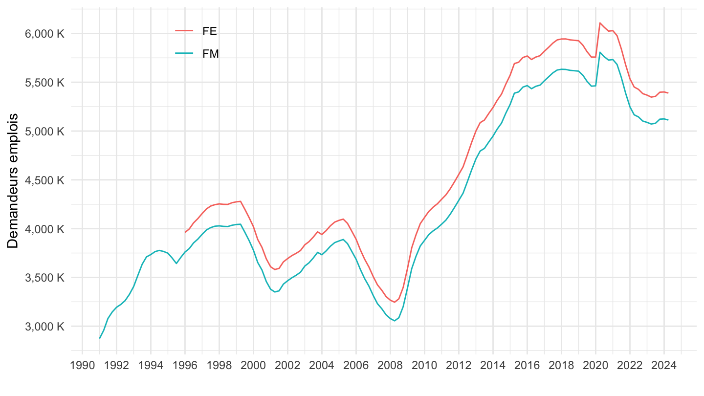
`DEMANDES-EMPLOIS-NATIONALES` |>
  filter(INDICATEUR == "DEMANDEURS_EMPLOI_PE",
         DEMANDEURS_EMPLOI %in% c("A", "B", "C", "A-B-C"),
         METIER == "SO",
         SEXE == "0",
         FREQ == "T",
         CORRECTION == "CVS-CJO",
         ANCIENNETE == "SO",
         DIPLOME == "SO",
         REF_AREA == "FM",
         AGE == "00-") |>
  quarter_to_date() |>
  mutate(OBS_VALUE = OBS_VALUE |> as.numeric()) |>

  ggplot() + theme_minimal() + xlab("") + ylab("Demandeurs emplois") +
  geom_line(aes(x = date, y = OBS_VALUE, color = DEMANDEURS_EMPLOI)) +
  scale_x_date(breaks = seq(1960, 2100, 2) |> paste0("-01-01") |> as.Date(),
               labels = date_format("%Y")) +
  scale_y_continuous(breaks = seq(0, 6000, 500),
                     labels = dollar_format(accuracy = 1, prefix = "", su = " K")) +
  theme(legend.position = c(0.3, 0.9),
        legend.title = element_blank())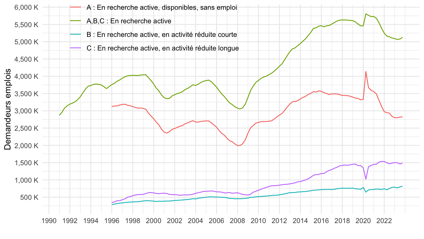
`DEMANDES-EMPLOIS-NATIONALES` |>
  filter(INDICATEUR == "DEMANDEURS_EMPLOI_PE",
         DEMANDEURS_EMPLOI %in% c("A", "B", "C", "A-B-C"),
         METIER == "SO",
         SEXE == "0",
         FREQ == "T",
         CORRECTION == "CVS-CJO",
         ANCIENNETE == "SO",
         DIPLOME == "SO",
         REF_AREA == "FM",
         AGE == "00-") |>
  quarter_to_date() |>
  filter(date >= as.Date("2005-01-01")) |>

  ggplot() + theme_minimal() + xlab("") + ylab("Demandeurs emplois") +
  geom_line(aes(x = date, y = OBS_VALUE, color = DEMANDEURS_EMPLOI)) +
  scale_x_date(breaks = seq(1960, 2100, 2) |> paste0("-01-01") |> as.Date(),
               labels = date_format("%Y")) +
  scale_y_continuous(breaks = seq(0, 6000, 500),
                     labels = dollar_format(accuracy = 1, prefix = "", su = " K")) +

  theme(legend.position = c(0.25, 0.9),
        legend.title = element_blank())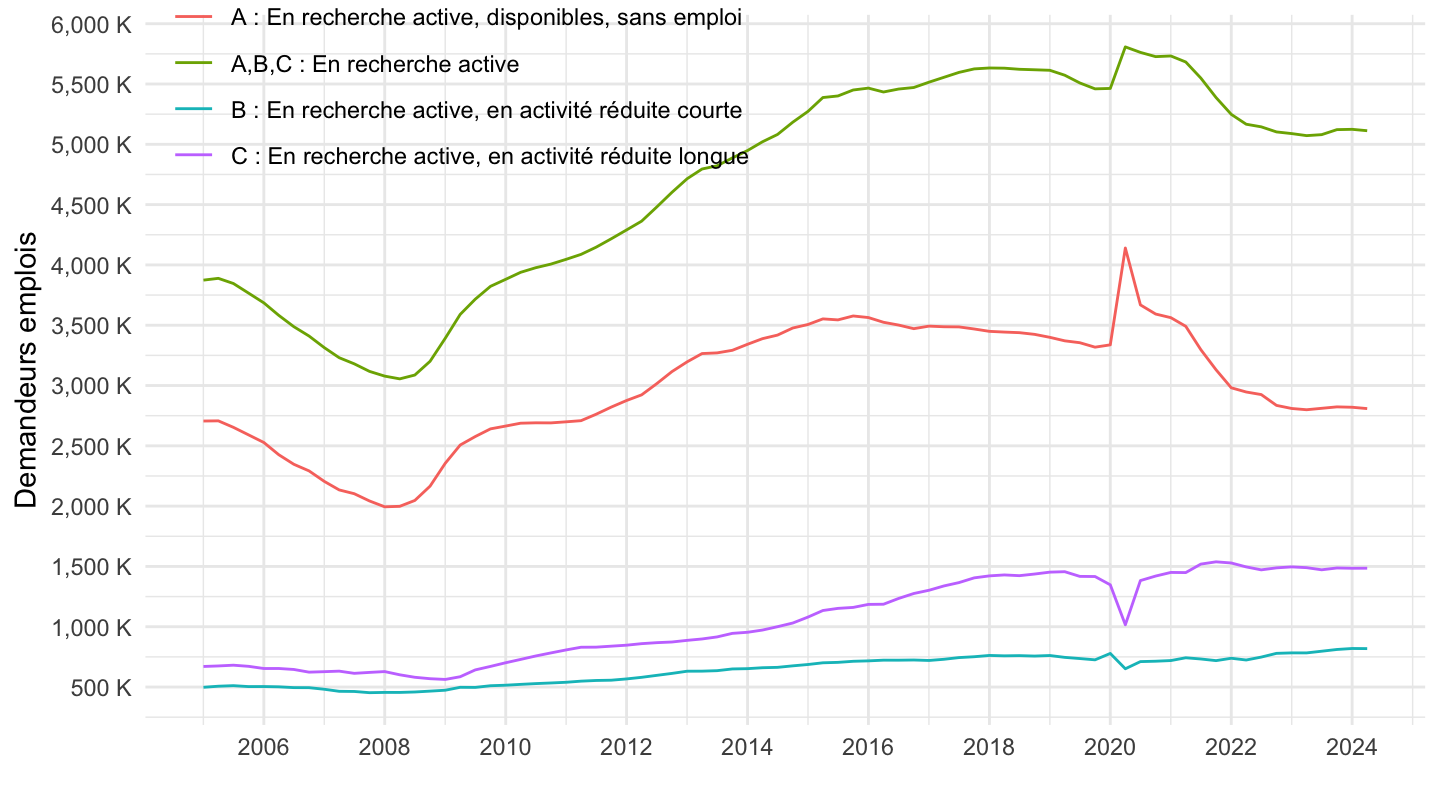
`DEMANDES-EMPLOIS-NATIONALES` |>
  filter(INDICATEUR == "DEMANDEURS_EMPLOI_PE",
         DEMANDEURS_EMPLOI == "A-B-C",
         METIER == "SO",
         SEXE == "0",
         FREQ == "T",
         CORRECTION == "CVS-CJO",
         ANCIENNETE == "SO",
         DIPLOME == "SO",
         REF_AREA == "FM",
         AGE %in% c("00-", "25-49", "50-", "00-24")) |>
  quarter_to_date() |>

  ggplot() + theme_minimal() + xlab("") + ylab("Demandeurs emplois") +
  geom_line(aes(x = date, y = OBS_VALUE, color = AGE)) +
  scale_x_date(breaks = seq(1960, 2100, 2) |> paste0("-01-01") |> as.Date(),
               labels = date_format("%Y")) +
  scale_y_log10(breaks = seq(0, 6000, 500),
                     labels = dollar_format(accuracy = 1, prefix = "", su = " K")) +

  theme(legend.position = c(0.3, 0.5),
        legend.title = element_blank())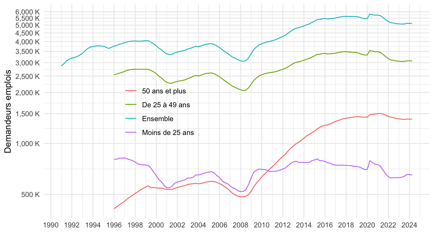
`DEMANDES-EMPLOIS-NATIONALES` |>
  filter(INDICATEUR == "DEMANDEURS_EMPLOI_PE",
         DEMANDEURS_EMPLOI == "A-B-C",
         METIER == "SO",
         SEXE == "0",
         FREQ == "T",
         CORRECTION == "CVS-CJO",
         ANCIENNETE == "SO",
         DIPLOME == "SO",
         REF_AREA == "FM",
         AGE %in% c("00-24")) |>
  quarter_to_date() |>

  ggplot() + theme_minimal() + xlab("") + ylab("Demandeurs emplois") +
  geom_line(aes(x = date, y = OBS_VALUE, color = AGE)) +
  scale_x_date(breaks = seq(1960, 2100, 2) |> paste0("-01-01") |> as.Date(),
               labels = date_format("%Y")) +
  scale_y_log10(breaks = seq(0, 6000, 100),
                     labels = dollar_format(accuracy = 1, prefix = "", su = " K")) +

  theme(legend.position = c(0.3, 0.5),
        legend.title = element_blank())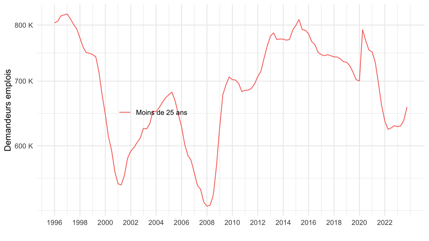
`DEMANDES-EMPLOIS-NATIONALES` |>
  filter(AGE == "00-29",
         DIPLOME %in% c("1-2", "3", "4", "5"),
         FREQ == "M") |>
  month_to_date() |>
  mutate(OBS_VALUE = OBS_VALUE |> as.numeric()) |>

  filter(!is.nan(OBS_VALUE)) |>
  ggplot() + theme_minimal() + xlab("") + ylab("Demandeurs emplois") +
  geom_line(aes(x = date, y = OBS_VALUE, color = DIPLOME)) +
  scale_x_date(breaks = seq(1960, 2100, 2) |> paste0("-01-01") |> as.Date(),
               labels = date_format("%Y")) +
  scale_y_continuous(breaks = seq(0, 6000, 100),
                labels = dollar_format(accuracy = 1, prefix = "", su = " K")) +

  theme(legend.position = c(0.5, 0.9),
        legend.title = element_blank())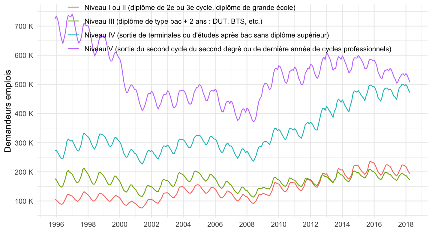
`DEMANDES-EMPLOIS-NATIONALES` |>
  filter(DIPLOME %in% c("1-2"),
         FREQ == "M") |>
  month_to_date() |>

  filter(!is.nan(OBS_VALUE)) |>
  ggplot() + theme_minimal() + xlab("") + ylab("Demandeurs emplois") +
  geom_line(aes(x = date, y = OBS_VALUE, color = AGE)) +
  scale_x_date(breaks = seq(1960, 2100, 2) |> paste0("-01-01") |> as.Date(),
               labels = date_format("%Y")) +
  scale_y_continuous(breaks = seq(50, 500, 25),
                     labels = dollar_format(accuracy = 1, prefix = "", su = " K")) +

  theme(legend.position = c(0.2, 0.9),
        legend.title = element_blank())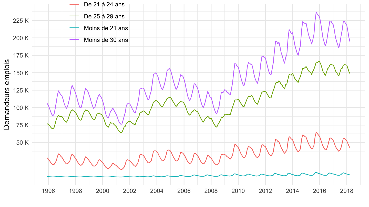
| source | dataset | Title | Updated |
|---|---|---|---|
| source | dataset | Title | Updated |
|---|---|---|---|
| source | dataset | Title | Updated |
|---|---|---|---|


