Revalorisation du Régime général de la caisse nationale d’assurance vieillesse (CNAV) - revalorisation_pension

Name: Revalorisation du Régime général de la caisse nationale d'assurance vieillesse (CNAV)
Creator: François Geerolf
License: https://www.etalab.gouv.fr/licence-ouverte-open-licence/

Données - IPP

Auteur

François Geerolf

Base 100

All

Lineaire

Code

revalorisation_pension |>
  select(date, index) |>
  gather(variable, value, -date) |>
  group_by(variable) |>
  complete(date = seq.Date(min(date), max(date), by = "day")) |>
  fill(value) |>
  mutate(value = 100*value/value[1]) |>
  ggplot() + geom_line(aes(x = date, y = value)) +
  theme_minimal() +
  scale_x_date(breaks = seq(1920, 2100, 5) |> paste0("-01-01") |> as.Date(),
               labels = date_format("%Y")) +
  theme(legend.position = c(0.3, 0.8),
        legend.title = element_blank()) +
  scale_y_continuous(breaks = seq(100, 20000, 500)) +
  ylab("Point Indice Fonction Publique") + xlab("")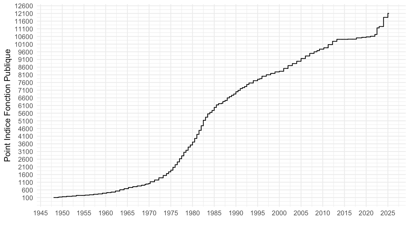

Log

Code

revalorisation_pension |>
  select(date, index) |>
  gather(variable, value, -date) |>
  group_by(variable) |>
  complete(date = seq.Date(min(date), max(date), by = "day")) |>
  fill(value) |>
  mutate(value = 100*value/value[1]) |>
  ggplot() + geom_line(aes(x = date, y = value)) +
  theme_minimal() +
  scale_x_date(breaks = seq(1920, 2100, 5) |> paste0("-01-01") |> as.Date(),
               labels = date_format("%Y")) +
  theme(legend.position = c(0.3, 0.8),
        legend.title = element_blank()) +
  scale_y_log10(breaks = c(100,200, 500, 800, 1000, 2000, 5000, 8000, 10000, 20000)) +
  ylab("Point Indice Fonction Publique") + xlab("")

1996-

nominal

Code

revalorisation_pension |>
  select(date, index) |>
  gather(variable, value, -date) |>
  group_by(variable) |>
  complete(date = seq.Date(min(date), max(date), by = "day")) |>
  fill(value) |>
  filter(date >= as.Date("1996-01-01")) |>
  mutate(value = 100*value/value[1]) |>
  ggplot() + geom_line(aes(x = date, y = value)) +
  theme_minimal() +
  scale_x_date(breaks = seq(1999, 2100, 5) |> paste0("-01-01") |> as.Date(),
               labels = date_format("%Y")) +
  theme(legend.position = c(0.3, 0.8),
        legend.title = element_blank()) +
  scale_y_log10(breaks = seq(0, 3000, 5)) +
  ylab("Pensions") + xlab("")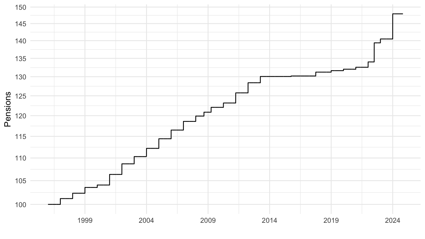

reel

Code

revalorisation_pension |>
  select(date, index) |>
  gather(variable, value, -date) |>
  group_by(variable) |>
  complete(date = seq.Date(min(date), max(date), by = "day")) |>
  fill(value) |>
  ungroup() |>
  left_join(cpi2_m, by = "date") |>
  filter(day(date) == 1) |>
  filter(date >= as.Date("1996-02-01")) |>
  transmute(date,
            `Retraites vs. 1996 (IPCH, Eurostat)` = (value/value[1])*(cpih[1]/cpih)-1,
            `Retraites vs. 1996 (IPC, INSEE)` = (value/value[1])*(cpi[1]/cpi)-1) |>
  gather(variable, OBS_VALUE, -date) |>
  ggplot() + geom_line(aes(x = date, y = OBS_VALUE, color = variable), size = 1) + theme_minimal() +
  scale_x_date(breaks = seq(1996, 2100, 5) |> paste0("-01-01") |> as.Date(),
               labels = date_format("%Y")) +
  theme(legend.position = c(0.43, 0.12),
        legend.title = element_blank()) +
  scale_y_continuous(breaks = 0.01*seq(-200, 200, 1),
                     labels = percent_format(acc = 1)) + 
  ylab("Retraites vs. 1996") + xlab("") +
  geom_label(data = . %>% filter(date == max(date)),
            aes(x = date, y = OBS_VALUE, label = percent(OBS_VALUE, acc = 0.1), color = variable), 
                  fontface ="bold", size = 3, show.legend = F) +
  scale_color_manual(values = viridis(3)[1:2]) +
  labs(title = "Niveau des retraites vs. 1996",
       subtitle = "Selon l'IPC préféré par l'Insee, et l'IPCH préféré par Eurostat")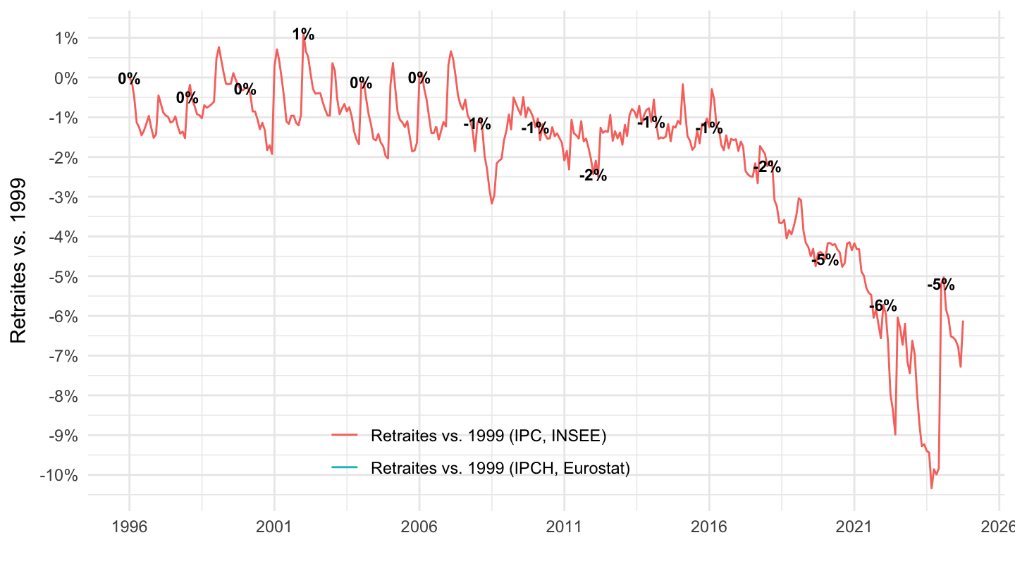

1999-

nominal

Code

revalorisation_pension |>
  select(date, index) |>
  gather(variable, value, -date) |>
  group_by(variable) |>
  complete(date = seq.Date(min(date), max(date), by = "day")) |>
  fill(value) |>
  filter(date >= as.Date("1999-01-01")) |>
  mutate(value = 100*value/value[1]) |>
  ggplot() + geom_line(aes(x = date, y = value)) +
  theme_minimal() +
  scale_x_date(breaks = seq(1999, 2100, 5) |> paste0("-01-01") |> as.Date(),
               labels = date_format("%Y")) +
  theme(legend.position = c(0.3, 0.8),
        legend.title = element_blank()) +
  scale_y_log10(breaks = seq(0, 3000, 5)) +
  ylab("Pensions") + xlab("")

reel

Code

revalorisation_pension |>
  select(date, index) |>
  gather(variable, value, -date) |>
  group_by(variable) |>
  complete(date = seq.Date(min(date), max(date), by = "day")) |>
  fill(value) |>
  filter(date >= as.Date("1999-01-01")) |>
  ungroup() |>
  left_join(cpi2_m, by = "date") |>
  filter(day(date) == 1) |>
  filter(date >= as.Date("1999-01-01")) |>
  transmute(date,
            `Retraites vs. 1999 (IPCH, Eurostat)` = (value/value[1])*(cpih[1]/cpih)-1,
            `Retraites vs. 1999 (IPC, INSEE)` = (value/value[1])*(cpi[1]/cpi)-1) |>
  gather(variable, OBS_VALUE, -date) |>
  ggplot() + geom_line(aes(x = date, y = OBS_VALUE, color = variable)) + theme_minimal() +
  scale_x_date(breaks = seq(1999, 2100, 5) |> paste0("-01-01") |> as.Date(),
               labels = date_format("%Y")) +
  theme(legend.position = c(0.43, 0.12),
        legend.title = element_blank()) +
  scale_y_continuous(breaks = 0.01*seq(-200, 200, 2),
                     labels = percent_format(acc = 1)) + 
  ylab("Retraites vs. 1999") + xlab("") +
  geom_text(data = . %>% filter((year(date) %in% seq(1999, 2020, 5) &
                                month(date) == 1) | (date == max(date))),
            aes(x = date, y = OBS_VALUE, label = percent(OBS_VALUE, acc = 1)), 
                  fontface ="bold", color = "black", size = 3) +
  geom_label(data = . %>% filter(max(date) == date),
             aes(x = date, y = OBS_VALUE, label = percent(OBS_VALUE, acc = 1), color = variable), show.legend = F)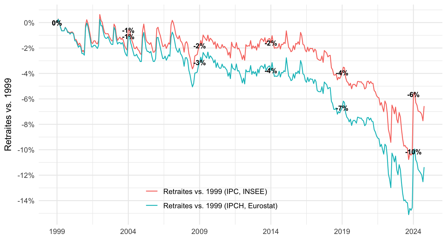

Décembre 2007-

nominal

Code

revalorisation_pension |>
  select(date, index) |>
  gather(variable, value, -date) |>
  group_by(variable) |>
  complete(date = seq.Date(min(date), max(date), by = "day")) |>
  fill(value) |>
  filter(date >= as.Date("2007-12-01")) |>
  mutate(value = 100*value/value[1]) |>
  ggplot() + geom_line(aes(x = date, y = value)) +
  theme_minimal() +
  scale_x_date(breaks = seq(2008, 2100, 2) |> paste0("-01-01") |> as.Date(),
               labels = date_format("%Y")) +
  theme(legend.position = c(0.3, 0.8),
        legend.title = element_blank()) +
  scale_y_log10(breaks = seq(0, 3000, 5)) +
  ylab("Pensions") + xlab("") + 
  geom_label(data = . %>% tail(1), aes(x = date, y = value, label = round(value, 1)))

2008-

nominal

Code

revalorisation_pension |>
  select(date, index) |>
  gather(variable, value, -date) |>
  group_by(variable) |>
  complete(date = seq.Date(min(date), max(date), by = "day")) |>
  fill(value) |>
  filter(date >= as.Date("2008-01-01")) |>
  mutate(value = 100*value/value[1]) |>
  ggplot() + geom_line(aes(x = date, y = value)) +
  theme_minimal() +
  scale_x_date(breaks = seq(2008, 2100, 2) |> paste0("-01-01") |> as.Date(),
               labels = date_format("%Y")) +
  theme(legend.position = c(0.3, 0.8),
        legend.title = element_blank()) +
  scale_y_log10(breaks = seq(0, 3000, 5)) +
  ylab("Pensions") + xlab("") + 
  geom_label(data = . %>% tail(1), aes(x = date, y = value, label = round(value, 1)))

Réel

Code

revalorisation_pension |>
  select(date, index) |>
  gather(variable, value, -date) |>
  group_by(variable) |>
  complete(date = seq.Date(min(date), max(date), by = "day")) |>
  fill(value) |>
  filter(date >= as.Date("2007-12-01")) |>
  ungroup() |>
  left_join(cpi2_m, by = "date") |>
  filter(day(date) == 1) |>
  filter(date >= as.Date("2007-12-01")) |>
  transmute(date,
            `Retraites vs. 2008 (IPCH, Eurostat)` = (value/value[1])*(cpih[1]/cpih)-1,
            `Retraites vs. 2008 (IPC, INSEE)` = (value/value[1])*(cpi[1]/cpi)-1) |>
  gather(variable, OBS_VALUE, -date) |>
  ggplot() + geom_line(aes(x = date, y = OBS_VALUE, color = variable)) + theme_minimal() +
  scale_x_date(breaks = seq(2008, 2100, 2) |> paste0("-01-01") |> as.Date(),
               labels = date_format("%Y")) +
  theme(legend.position = c(0.43, 0.12),
        legend.title = element_blank()) +
  scale_y_continuous(breaks = 0.01*seq(-200, 200, 1),
                     labels = percent_format(acc = 1)) + 
  ylab("Retraites vs. 1999") + xlab("") +
  geom_text(data = . %>% filter(date %in% c(as.Date("2014-01-01"),
                                            as.Date("2017-04-01"),
                                            max(date))),
            aes(x = date, y = OBS_VALUE, label = percent(OBS_VALUE, acc = 0.1)), 
                  fontface ="bold", color = "black", size = 3)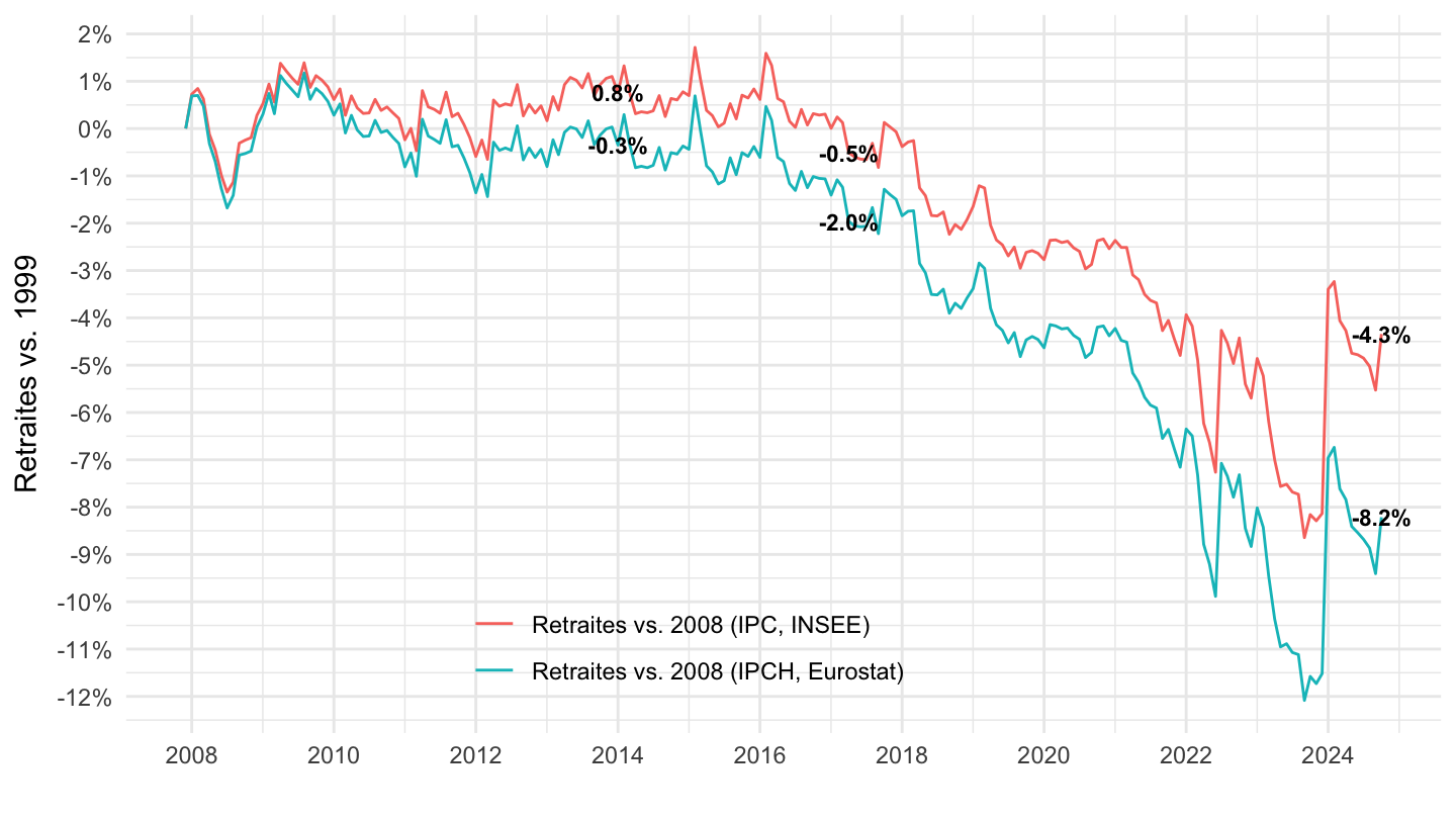

2017-

nominal

Code

revalorisation_pension |>
  select(date, index) |>
  gather(variable, value, -date) |>
  group_by(variable) |>
  complete(date = seq.Date(min(date), max(date), by = "day")) |>
  fill(value) |>
  filter(date >= as.Date("2017-01-01")) |>
  mutate(value = 100*value/value[1]) |>
  ggplot() + geom_line(aes(x = date, y = value)) +
  theme_minimal() +
  scale_x_date(breaks = seq(2017, 2100, 1) |> paste0("-01-01") |> as.Date(),
               labels = date_format("%Y")) +
  theme(legend.position = c(0.3, 0.8),
        legend.title = element_blank()) +
  scale_y_log10(breaks = seq(0, 3000, 5)) +
  ylab("Pensions") + xlab("") + 
  geom_label(data = . %>% tail(1), aes(x = date, y = value, label = round(value, 1)))

Réel

Code

revalorisation_pension |>
  select(date, index) |>
  gather(variable, value, -date) |>
  group_by(variable) |>
  complete(date = seq.Date(min(date), max(date), by = "day")) |>
  fill(value) |>
  filter(date >= as.Date("2017-01-01")) |>
  ungroup() |>
  left_join(cpi2_m, by = "date") |>
  filter(day(date) == 1) |>
  filter(date >= as.Date("2007-01-01")) |>
  transmute(date,
            `Retraites vs. 2017 (IPCH, Eurostat)` = (value/value[1])*(cpih[1]/cpih)-1,
            `Retraites vs. 2017 (IPC, INSEE)` = (value/value[1])*(cpi[1]/cpi)-1) |>
  gather(variable, OBS_VALUE, -date) |>
  ggplot() + geom_line(aes(x = date, y = OBS_VALUE, color = variable)) + theme_minimal() +
  scale_x_date(breaks = seq(2008, 2100, 1) |> paste0("-01-01") |> as.Date(),
               labels = date_format("%Y")) +
  theme(legend.position = c(0.43, 0.12),
        legend.title = element_blank()) +
  scale_y_continuous(breaks = 0.01*seq(-200, 200, 1),
                     labels = percent_format(acc = 1)) + 
  ylab("Retraites vs. 1999") + xlab("") +
  geom_text(data = . %>% filter(date %in% c(as.Date("2014-01-01"),
                                            as.Date("2017-04-01"))),
            aes(x = date, y = OBS_VALUE, label = percent(OBS_VALUE, acc = 0.1)), 
                  fontface ="bold", color = "black", size = 3) +
  geom_label(data = . %>% filter(max(date) == date),
             aes(x = date, y = OBS_VALUE, label = percent(OBS_VALUE, acc = 1), color = variable), show.legend = F)

2021-

nominal

Code

revalorisation_pension |>
  select(date, index) |>
  gather(variable, value, -date) |>
  group_by(variable) |>
  complete(date = seq.Date(min(date), max(date), by = "day")) |>
  fill(value) |>
  filter(date >= as.Date("2021-01-01")) |>
  mutate(value = 100*value/value[1]) |>
  ggplot() + geom_line(aes(x = date, y = value)) +
  theme_minimal() +
  scale_x_date(breaks = seq(2017, 2100, 1) |> paste0("-01-01") |> as.Date(),
               labels = date_format("%Y")) +
  theme(legend.position = c(0.3, 0.8),
        legend.title = element_blank()) +
  scale_y_log10(breaks = seq(0, 3000, 2)) +
  ylab("Pensions") + xlab("") + 
  geom_label(data = . %>% tail(1), aes(x = date, y = value, label = round(value, 1)))

Réel

Code

revalorisation_pension |>
  select(date, index) |>
  gather(variable, value, -date) |>
  group_by(variable) |>
  complete(date = seq.Date(min(date), max(date), by = "day")) |>
  fill(value) |>
  filter(date >= as.Date("2021-01-01")) |>
  ungroup() |>
  left_join(cpi2_m, by = "date") |>
  filter(day(date) == 1) |>
  filter(date >= as.Date("2021-01-01")) |>
  transmute(date,
            `Retraites vs. 2021 (IPCH, Eurostat)` = (value/value[1])*(cpih[1]/cpih)-1,
            `Retraites vs. 2021 (IPC, INSEE)` = (value/value[1])*(cpi[1]/cpi)-1) |>
  gather(variable, OBS_VALUE, -date) |>
  ggplot() + geom_line(aes(x = date, y = OBS_VALUE, color = variable)) + theme_minimal() +
  scale_x_date(breaks = seq(2008, 2100, 1) |> paste0("-01-01") |> as.Date(),
               labels = date_format("%Y")) +
  theme(legend.position = c(0.25, 0.12),
        legend.title = element_blank()) +
  scale_y_continuous(breaks = 0.01*seq(-200, 200, 1),
                     labels = percent_format(acc = 1)) + 
  ylab("Retraites vs. 2021") + xlab("") +
  geom_label(data = . %>% filter(date %in% c(as.Date("2014-01-01"),
                                            as.Date("2017-04-01"),
                                            max(date))),
            aes(x = date, y = OBS_VALUE, label = percent(OBS_VALUE, acc = 0.1), color = variable), 
                  fontface ="bold", size = 3, show.legend = F)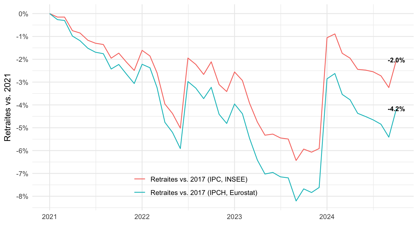

1999-

Retraites

Code

data1 <- revalorisation_pension |>
  select(date, index) |>
  gather(variable, value, -date) |>
  group_by(variable) |>
  complete(date = seq.Date(min(date), max(date), by = "day")) |>
  fill(value) |>
  filter(date >= as.Date("1999-01-01")) |>
  ungroup() |>
  left_join(cpi2_m, by = "date") |>
  filter(day(date) == 1) |>
  filter(date >= as.Date("1999-01-01")) |>
  transmute(date,
            `IPCH, Eurostat` = (value/value[1])*(cpih[1]/cpih),
            `IPC, INSEE` = (value/value[1])*(cpi[1]/cpi)) |>
  gather(type, OBS_VALUE, -date) |>
  mutate(variable = "Retraites vs. 1999")

data1 |>
  ggplot() + geom_line(aes(x = date, y = OBS_VALUE, linetype = type)) + theme_minimal() +
  scale_x_date(breaks = seq(1999, 2100, 5) |> paste0("-01-01") |> as.Date(),
               labels = date_format("%Y")) +
  theme(legend.position = c(0.43, 0.12),
        legend.title = element_blank()) +
  scale_y_log10(breaks = seq(1, 0.02, -0.02),
                labels = percent(seq(1, 0.02, -0.02)-1, acc = 1)) + 
  ylab("Retraites vs. 1999") + xlab("") +
  geom_text(data = . %>% filter((year(date) %in% seq(1999, 2040, 5) & month(date) == 1) | (max(date) == date)),
            aes(x = date, y = OBS_VALUE, label = percent(OBS_VALUE-1, acc = 0.1)), 
                  fontface ="bold", color = "black", size = 3)

Indice Fonction Publique

Code

net_brut_mensuel <- read_parquet(here::here("data", "insee", "INDICE-TRAITEMENT-FP-net-brut-mensuel.parquet"))
data2 <- indicefp |>
  select(date, point_indice_en_euros) |>
  arrange(desc(date)) |>
  gather(variable, value, -date) |>
  group_by(variable) |>
  complete(date = seq.Date(min(date), max(date), by = "day")) |>
  fill(value) |>
  ungroup() |>
  left_join(cpi2_m, by = "date") |>
  filter(day(date) == 1) |>
  left_join(net_brut_mensuel, by = "date") |>
  filter(date >= as.Date("1999-01-01")) |>
  transmute(date,
            `IPCH, Eurostat` = (value/value[1])*(cpih[1]/cpih)*(net_brut/net_brut[1]),
            `IPC, INSEE` = (value/value[1])*(cpi[1]/cpi)*(net_brut/net_brut[1])) |>
  gather(type, OBS_VALUE, -date) |>
  mutate(variable = "Point d'Indice de la Fonction Publique vs. 1999")

data2 |>
  ggplot() + geom_line(aes(x = date, y = OBS_VALUE, linetype = type)) + theme_minimal() +
  scale_x_date(breaks = c(seq(1999, 2100, 5), seq(1997, 2100, 5)) |> paste0("-01-01") |> as.Date(),
               labels = date_format("%Y")) +
  theme(legend.position = c(0.43, 0.12),
        legend.title = element_blank()) +
  scale_y_log10(breaks = seq(1, 0.02, -0.02),
                labels = percent(seq(1, 0.02, -0.02)-1, acc = 1)) + 
  ylab("Point Indice Fonction Publique vs. 1999") + xlab("") +
  geom_text(data = . %>% filter(year(date) %in% seq(1999, 2040, 5),
                                month(date) == 1),
            aes(x = date, y = OBS_VALUE, label = percent(OBS_VALUE-1, acc = 0.1)), 
                  fontface ="bold", color = "black", size = 3)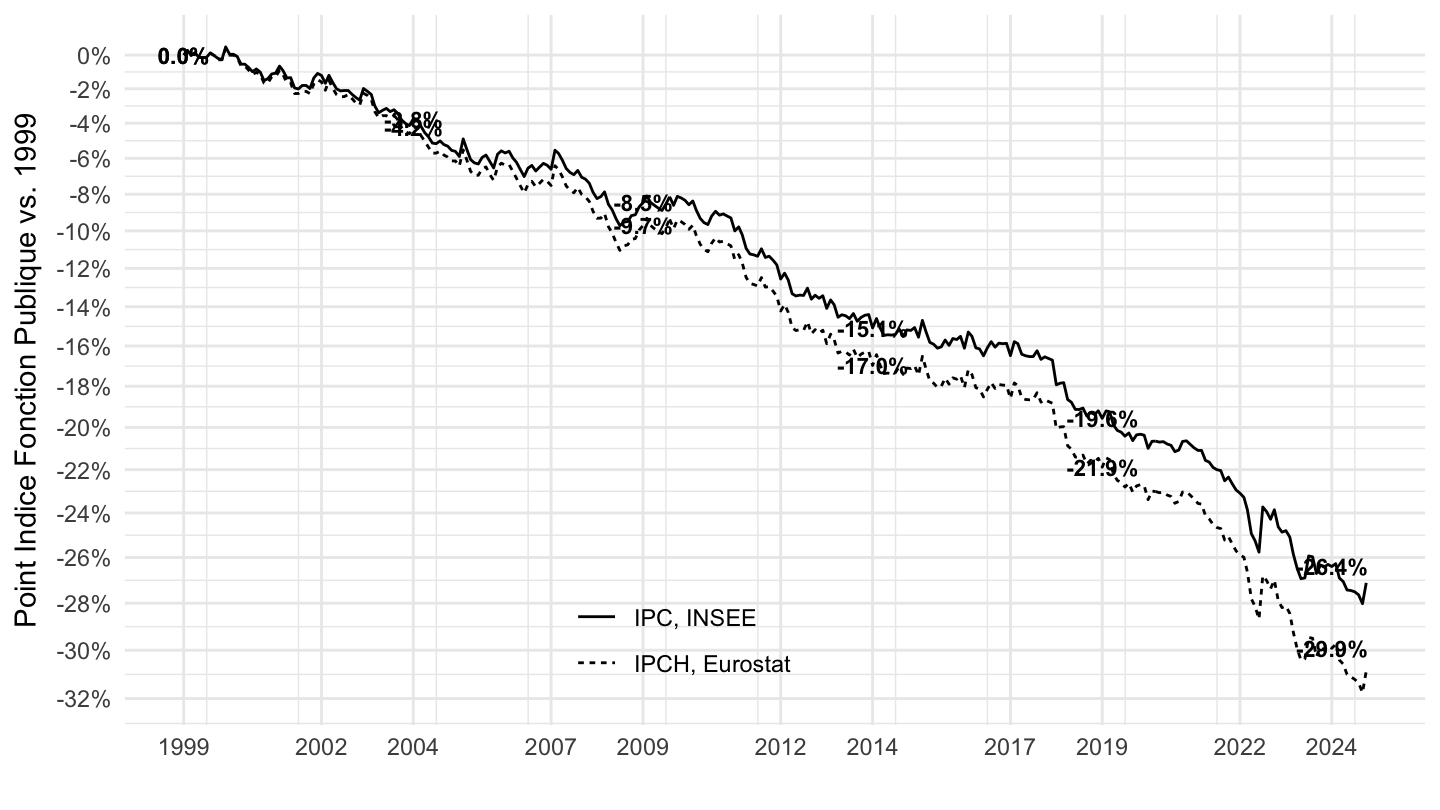

Merge

Code

data2 |>
  bind_rows(data1) |>
  mutate(variable = factor(variable, levels = c("Retraites vs. 1999",
                                                "Point d'Indice de la Fonction Publique vs. 1999"))) |>
  ggplot() + geom_line(aes(x = date, y = OBS_VALUE,  color = variable, linetype = type)) + theme_minimal() +
  scale_linetype_manual(values = c("dashed", "solid")) +
  scale_x_date(breaks = c(seq(1999, 2100, 5), seq(1997, 2100, 5)) |> paste0("-01-01") |> as.Date(),
               labels = date_format("%Y")) +
  theme(legend.position = c(0.32, 0.25),
        legend.title = element_blank(),
        legend.key.size = unit(0.5, "cm")) +
  scale_y_log10(breaks = seq(1, 0.02, -0.02),
                labels = percent(seq(1, 0.02, -0.02)-1, acc = 1)) + 
  ylab("Valeur vs. 1999") + xlab("") +
  geom_text(data = . %>% filter(date == max(date)),
            aes(x = date, y = OBS_VALUE, label = percent(OBS_VALUE-1, acc = 1), color = variable), 
                  fontface ="bold", size = 3, show.legend = F)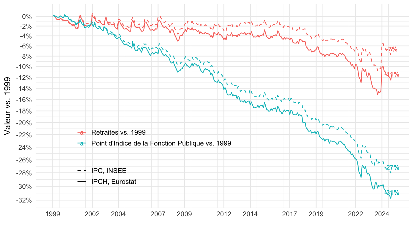

2007-12-

Retraites

Code

data1 <- revalorisation_pension |>
  select(date, index) |>
  gather(variable, value, -date) |>
  group_by(variable) |>
  complete(date = seq.Date(min(date), max(date), by = "day")) |>
  fill(value) |>
  filter(date >= as.Date("2007-12-01")) |>
  ungroup() |>
  left_join(cpi2_m, by = "date") |>
  filter(day(date) == 1) |>
  filter(date >= as.Date("2007-12-01")) |>
  transmute(date,
            `IPCH, Eurostat` = (value/value[1])*(cpih[1]/cpih),
            `IPC, INSEE` = (value/value[1])*(cpi[1]/cpi)) |>
  gather(type, OBS_VALUE, -date) |>
  mutate(variable = "Retraites vs. 2008")

data1 |>
  ggplot() + geom_line(aes(x = date, y = OBS_VALUE, linetype = type)) + theme_minimal() +
  scale_x_date(breaks = seq(1999, 2100, 2) |> paste0("-01-01") |> as.Date(),
               labels = date_format("%Y")) +
  theme(legend.position = c(0.43, 0.12),
        legend.title = element_blank()) +
  scale_y_log10(breaks = seq(1, 0.02, -0.02),
                labels = percent(seq(1, 0.02, -0.02)-1, acc = 1)) + 
  ylab("Retraites vs. 2008") + xlab("") +
  geom_text(data = . %>% filter(year(date) %in% seq(1999, 2040, 5),
                                month(date) == 1),
            aes(x = date, y = OBS_VALUE, label = percent(OBS_VALUE-1, acc = 0.1)), 
                  fontface ="bold", color = "black", size = 3)

Indice Fonction Publique

Code

net_brut_mensuel <- read_parquet(here::here("data", "insee", "INDICE-TRAITEMENT-FP-net-brut-mensuel.parquet"))
data2 <- indicefp |>
  select(date, point_indice_en_euros) |>
  arrange(desc(date)) |>
  gather(variable, value, -date) |>
  group_by(variable) |>
  complete(date = seq.Date(min(date), max(date), by = "day")) |>
  fill(value) |>
  ungroup() |>
  left_join(cpi2_m, by = "date") |>
  filter(day(date) == 1) |>
  left_join(net_brut_mensuel, by = "date") |>
  filter(date >= as.Date("2007-12-01")) |>
  transmute(date,
            `IPCH, Eurostat` = (value/value[1])*(cpih[1]/cpih)*(net_brut/net_brut[1]),
            `IPC, INSEE` = (value/value[1])*(cpi[1]/cpi)*(net_brut/net_brut[1])) |>
  gather(type, OBS_VALUE, -date) |>
  mutate(variable = "Point d'Indice de la Fonction Publique vs. 2008")

data2 |>
  ggplot() + geom_line(aes(x = date, y = OBS_VALUE, linetype = type)) + theme_minimal() +
  scale_x_date(breaks = c(seq(1999, 2100, 5), seq(1997, 2100, 5)) |> paste0("-01-01") |> as.Date(),
               labels = date_format("%Y")) +
  theme(legend.position = c(0.43, 0.12),
        legend.title = element_blank()) +
  scale_y_log10(breaks = seq(1, 0.02, -0.02),
                labels = percent(seq(1, 0.02, -0.02)-1, acc = 1)) + 
  ylab("Point Indice Fonction Publique vs. 2008") + xlab("") +
  geom_text(data = . %>% filter(year(date) %in% seq(1999, 2040, 5),
                                month(date) == 1),
            aes(x = date, y = OBS_VALUE, label = percent(OBS_VALUE-1, acc = 0.1)), 
                  fontface ="bold", color = "black", size = 3)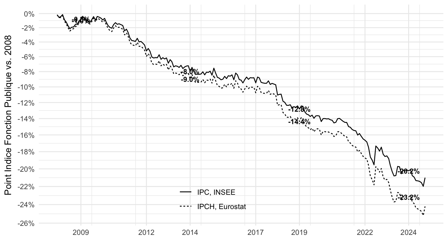

Merge

Code

data2 |>
  bind_rows(data1) |>
  mutate(variable = factor(variable, levels = c("Retraites vs. 2008",
                                                "Point d'Indice de la Fonction Publique vs. 2008"))) |>
  ggplot() + geom_line(aes(x = date, y = OBS_VALUE,  color = variable, linetype = type)) + theme_minimal() +
  scale_linetype_manual(values = c("dashed", "solid")) +
  scale_x_date(breaks = c(seq(1998, 2100, 2), seq(2008, 2100, 2)) |> paste0("-01-01") |> as.Date(),
               labels = date_format("%Y")) +
  theme(legend.position = c(0.32, 0.25),
        legend.title = element_blank(),
        legend.key.size = unit(0.5, "cm")) +
  scale_y_log10(breaks = seq(1, 0.02, -0.02),
                labels = percent(seq(1, 0.02, -0.02)-1, acc = 1)) + 
  ylab("Valeur vs. 2008") + xlab("") +
  geom_text(data = . %>% filter(date == max(date)),
            aes(x = date, y = OBS_VALUE, label = percent(OBS_VALUE-1, acc = 0.1)), 
                  fontface ="bold", color = "black", size = 3)

2010-

Retraites

Code

data1 <- revalorisation_pension |>
  select(date, index) |>
  gather(variable, value, -date) |>
  group_by(variable) |>
  complete(date = seq.Date(min(date), max(date), by = "day")) |>
  fill(value) |>
  filter(date >= as.Date("2010-01-01")) |>
  ungroup() |>
  left_join(cpi2_m, by = "date") |>
  filter(day(date) == 1) |>
  filter(date >= as.Date("2010-01-01")) |>
  transmute(date,
            `IPCH, Eurostat` = (value/value[1])*(cpih[1]/cpih),
            `IPC, INSEE` = (value/value[1])*(cpi[1]/cpi)) |>
  gather(type, OBS_VALUE, -date) |>
  mutate(variable = "Retraites vs. 2010")

data1 |>
  ggplot() + geom_line(aes(x = date, y = OBS_VALUE, linetype = type)) + theme_minimal() +
  scale_x_date(breaks = seq(1999, 2100, 1) |> paste0("-01-01") |> as.Date(),
               labels = date_format("%Y")) +
  theme(legend.position = c(0.43, 0.12),
        legend.title = element_blank()) +
  scale_y_log10(breaks = seq(1, 0.02, -0.02),
                labels = percent(seq(1, 0.02, -0.02)-1, acc = 1)) + 
  ylab("Retraites vs. 2010") + xlab("") +
  geom_text(data = . %>% filter(year(date) %in% seq(2010, 2040, 2),
                                month(date) == 1),
            aes(x = date, y = OBS_VALUE, label = percent(OBS_VALUE-1, acc = 0.1)), 
                  fontface ="bold", color = "black", size = 3)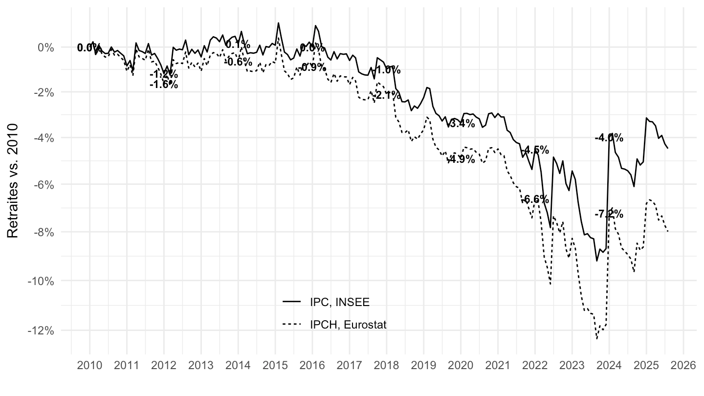

Indice Fonction Publique

Code

net_brut_mensuel <- read_parquet(here::here("data", "insee", "INDICE-TRAITEMENT-FP-net-brut-mensuel.parquet"))
data2 <- indicefp |>
  select(date, point_indice_en_euros) |>
  arrange(desc(date)) |>
  gather(variable, value, -date) |>
  group_by(variable) |>
  complete(date = seq.Date(min(date), max(date), by = "day")) |>
  fill(value) |>
  ungroup() |>
  left_join(cpi2_m, by = "date") |>
  filter(day(date) == 1) |>
  left_join(net_brut_mensuel, by = "date") |>
  filter(date >= as.Date("2010-01-01")) |>
  transmute(date,
            `IPCH, Eurostat` = (value/value[1])*(cpih[1]/cpih)*(net_brut/net_brut[1]),
            `IPC, INSEE` = (value/value[1])*(cpi[1]/cpi)*(net_brut/net_brut[1])) |>
  gather(type, OBS_VALUE, -date) |>
  mutate(variable = "Point d'Indice de la Fonction Publique vs. 2010")

data2 |>
  ggplot() + geom_line(aes(x = date, y = OBS_VALUE, linetype = type)) + theme_minimal() +
  scale_x_date(breaks = c(seq(1999, 2100, 2)) |> paste0("-01-01") |> as.Date(),
               labels = date_format("%Y")) +
  theme(legend.position = c(0.43, 0.12),
        legend.title = element_blank()) +
  scale_y_log10(breaks = seq(1, 0.02, -0.02),
                labels = percent(seq(1, 0.02, -0.02)-1, acc = 1)) + 
  ylab("Point Indice Fonction Publique vs. 2010") + xlab("") +
  geom_text(data = . %>% filter(year(date) %in% seq(2010, 2040, 2),
                                month(date) == 1),
            aes(x = date, y = OBS_VALUE, label = percent(OBS_VALUE-1, acc = 0.1)), 
                  fontface ="bold", color = "black", size = 3)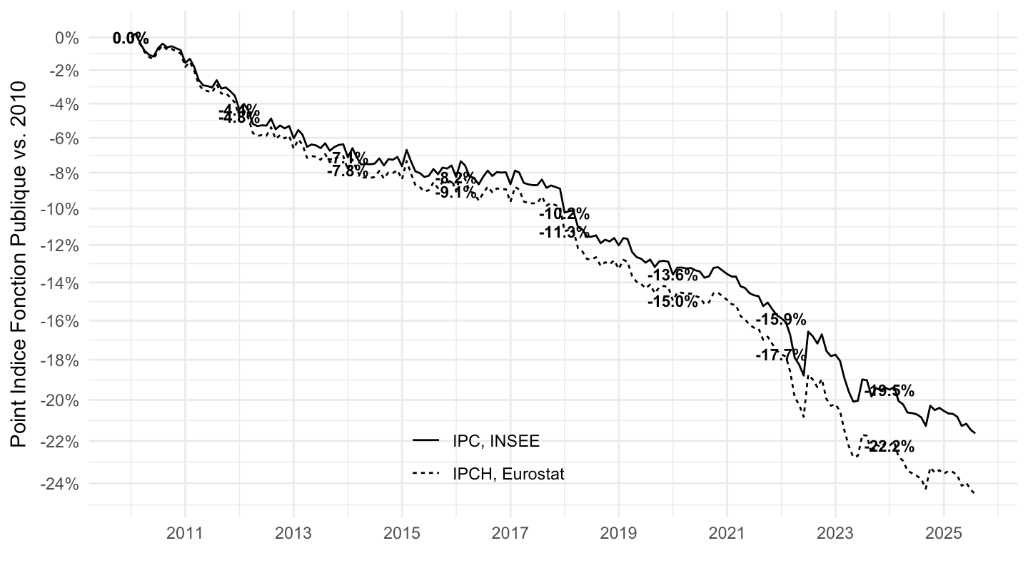

Merge

Code

data2 |>
  bind_rows(data1) |>
  mutate(variable = factor(variable, levels = c("Retraites vs. 2010",
                                                "Point d'Indice de la Fonction Publique vs. 2010"))) |>
  ggplot() + geom_line(aes(x = date, y = OBS_VALUE,  color = variable, linetype = type)) + theme_minimal() +
  scale_linetype_manual(values = c("dashed", "solid")) +
  scale_x_date(breaks = c(seq(1999, 2100, 1), seq(1997, 2100, 5)) |> paste0("-01-01") |> as.Date(),
               labels = date_format("%Y")) +
  theme(legend.position = c(0.32, 0.25),
        legend.title = element_blank(),
        legend.key.size = unit(0.5, "cm")) +
  scale_y_log10(breaks = seq(2, 0.02, -0.02),
                labels = percent(seq(2, 0.02, -0.02)-1, acc = 1)) + 
  ylab("Valeur vs. 2010") + xlab("") +
  geom_text(data = . %>% filter(date == max(date)),
            aes(x = date, y = OBS_VALUE, label = percent(OBS_VALUE-1, acc = 0.1), color = variable), 
                  fontface ="bold",  size = 3, show.legend = F)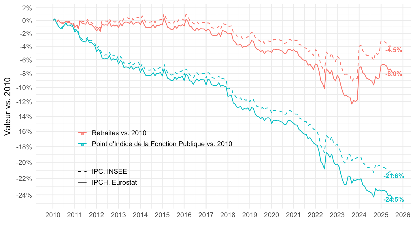

2012-

Merge

Code

data1 <- revalorisation_pension |>
  select(date, index) |>
  gather(variable, value, -date) |>
  group_by(variable) |>
  complete(date = seq.Date(min(date), max(date), by = "day")) |>
  fill(value) |>
  filter(date >= as.Date("2012-01-01")) |>
  ungroup() |>
  left_join(cpi2_m, by = "date") |>
  filter(day(date) == 1) |>
  filter(date >= as.Date("2012-01-01")) |>
  transmute(date,
            `IPCH, Eurostat` = (value/value[1])*(cpih[1]/cpih),
            `IPC, INSEE` = (value/value[1])*(cpi[1]/cpi)) |>
  gather(type, OBS_VALUE, -date) |>
  mutate(variable = "Retraites vs. 2012")

net_brut_mensuel <- read_parquet(here::here("data", "insee", "INDICE-TRAITEMENT-FP-net-brut-mensuel.parquet"))
data2 <- indicefp |>
  select(date, point_indice_en_euros) |>
  arrange(desc(date)) |>
  gather(variable, value, -date) |>
  group_by(variable) |>
  complete(date = seq.Date(min(date), max(date), by = "day")) |>
  fill(value) |>
  ungroup() |>
  left_join(cpi2_m, by = "date") |>
  filter(day(date) == 1) |>
  left_join(net_brut_mensuel, by = "date") |>
  filter(date >= as.Date("2012-01-01")) |>
  transmute(date,
            `IPCH, Eurostat` = (value/value[1])*(cpih[1]/cpih)*(net_brut/net_brut[1]),
            `IPC, INSEE` = (value/value[1])*(cpi[1]/cpi)*(net_brut/net_brut[1])) |>
  gather(type, OBS_VALUE, -date) |>
  mutate(variable = "Point d'Indice de la Fonction Publique vs. 2012")

data2 |>
  bind_rows(data1) |>
  mutate(variable = factor(variable, levels = c("Retraites vs. 2012",
                                                "Point d'Indice de la Fonction Publique vs. 2012"))) |>
  ggplot() + geom_line(aes(x = date, y = OBS_VALUE,  color = variable, linetype = type)) + theme_minimal() +
  scale_linetype_manual(values = c("dashed", "solid")) +
  scale_x_date(breaks = c(seq(1999, 2100, 1), seq(1997, 2100, 5)) |> paste0("-01-01") |> as.Date(),
               labels = date_format("%Y")) +
  theme(legend.position = c(0.32, 0.25),
        legend.title = element_blank(),
        legend.key.size = unit(0.5, "cm")) +
  scale_y_log10(breaks = seq(2, 0.02, -0.02),
                labels = percent(seq(2, 0.02, -0.02)-1, acc = 1)) + 
  ylab("Valeur vs. 2012") + xlab("") +
  geom_text(data = . %>% filter(date == max(date)),
            aes(x = date, y = OBS_VALUE, label = percent(OBS_VALUE-1, acc = 0.1), color = variable), 
                  fontface ="bold",  size = 3, show.legend = F)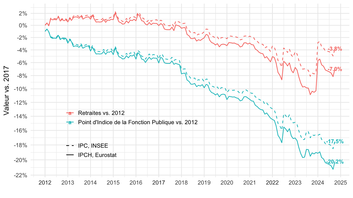

2017-

Retraites

Code

data1 <- revalorisation_pension |>
  select(date, index) |>
  gather(variable, value, -date) |>
  group_by(variable) |>
  complete(date = seq.Date(min(date), max(date), by = "day")) |>
  fill(value) |>
  filter(date >= as.Date("2017-01-01")) |>
  ungroup() |>
  left_join(cpi2_m, by = "date") |>
  filter(day(date) == 1) |>
  filter(date >= as.Date("2017-01-01")) |>
  transmute(date,
            `IPCH, Eurostat` = (value/value[1])*(cpih[1]/cpih),
            `IPC, INSEE` = (value/value[1])*(cpi[1]/cpi)) |>
  gather(type, OBS_VALUE, -date) |>
  mutate(variable = "Retraites vs. 2017")

data1 |>
  ggplot() + geom_line(aes(x = date, y = OBS_VALUE, linetype = type)) + theme_minimal() +
  scale_x_date(breaks = seq(1999, 2100, 1) |> paste0("-01-01") |> as.Date(),
               labels = date_format("%Y")) +
  theme(legend.position = c(0.43, 0.12),
        legend.title = element_blank()) +
  scale_y_log10(breaks = seq(1, 0.02, -0.02),
                labels = percent(seq(1, 0.02, -0.02)-1, acc = 1)) + 
  ylab("Retraites vs. 1999") + xlab("") +
  geom_text(data = . %>% filter(year(date) %in% seq(1999, 2040, 5),
                                month(date) == 1),
            aes(x = date, y = OBS_VALUE, label = percent(OBS_VALUE-1, acc = 0.1)), 
                  fontface ="bold", color = "black", size = 3)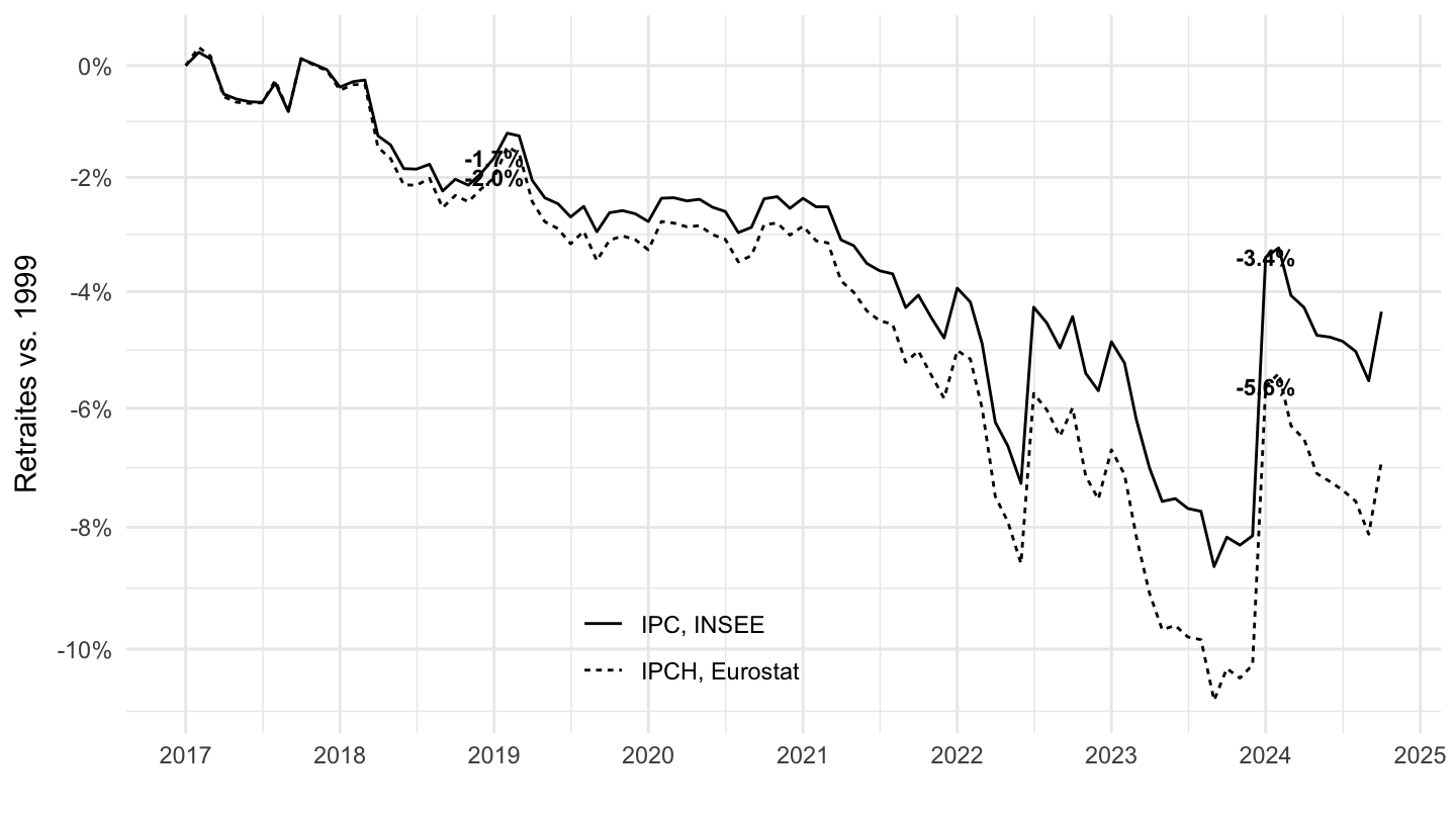

Indice Fonction Publique

Code

net_brut_mensuel <- read_parquet(here::here("data", "insee", "INDICE-TRAITEMENT-FP-net-brut-mensuel.parquet"))
data2 <- indicefp |>
  select(date, point_indice_en_euros) |>
  arrange(desc(date)) |>
  gather(variable, value, -date) |>
  group_by(variable) |>
  complete(date = seq.Date(min(date), max(date), by = "day")) |>
  fill(value) |>
  ungroup() |>
  left_join(cpi2_m, by = "date") |>
  filter(day(date) == 1) |>
  left_join(net_brut_mensuel, by = "date") |>
  filter(date >= as.Date("2017-01-01")) |>
  transmute(date,
            `IPCH, Eurostat` = (value/value[1])*(cpih[1]/cpih)*(net_brut/net_brut[1]),
            `IPC, INSEE` = (value/value[1])*(cpi[1]/cpi)*(net_brut/net_brut[1])) |>
  gather(type, OBS_VALUE, -date) |>
  mutate(variable = "Point d'Indice de la Fonction Publique vs. 2017")

data2 |>
  ggplot() + geom_line(aes(x = date, y = OBS_VALUE, linetype = type)) + theme_minimal() +
  scale_x_date(breaks = c(seq(1999, 2100, 5), seq(1997, 2100, 5)) |> paste0("-01-01") |> as.Date(),
               labels = date_format("%Y")) +
  theme(legend.position = c(0.43, 0.12),
        legend.title = element_blank()) +
  scale_y_log10(breaks = seq(1, 0.02, -0.02),
                labels = percent(seq(1, 0.02, -0.02)-1, acc = 1)) + 
  ylab("Point Indice Fonction Publique vs. 1999") + xlab("") +
  geom_text(data = . %>% filter(year(date) %in% seq(1999, 2040, 5),
                                month(date) == 1),
            aes(x = date, y = OBS_VALUE, label = percent(OBS_VALUE-1, acc = 0.1)), 
                  fontface ="bold", color = "black", size = 3)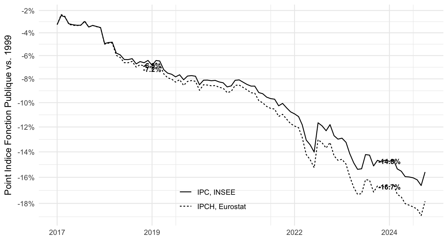

Merge

Code

data2 |>
  bind_rows(data1) |>
  mutate(variable = factor(variable, levels = c("Retraites vs. 2017",
                                                "Point d'Indice de la Fonction Publique vs. 2017"))) |>
  ggplot() + geom_line(aes(x = date, y = OBS_VALUE,  color = variable, linetype = type), linewidth = 1) + theme_minimal() +
  scale_linetype_manual(values = c("dotted", "solid")) +
  scale_x_date(breaks = c(seq(1999, 2100, 1), seq(1997, 2100, 5)) |> paste0("-01-01") |> as.Date(),
               labels = date_format("%Y")) +
  theme(legend.position = c(0.32, 0.25),
        legend.title = element_blank(),
        legend.key.size = unit(0.5, "cm")) +
  scale_y_log10(breaks = seq(1, 0.02, -0.02),
                labels = percent(seq(1, 0.02, -0.02)-1, acc = 1)) + 
  ylab("Valeur vs. 2017") + xlab("") +
  geom_label(data = . %>% filter(date == max(date)),
            aes(x = date, y = OBS_VALUE, label = percent(OBS_VALUE-1, acc = 0.1), color = variable), 
                  fontface ="bold",  size = 3, show.legend = F)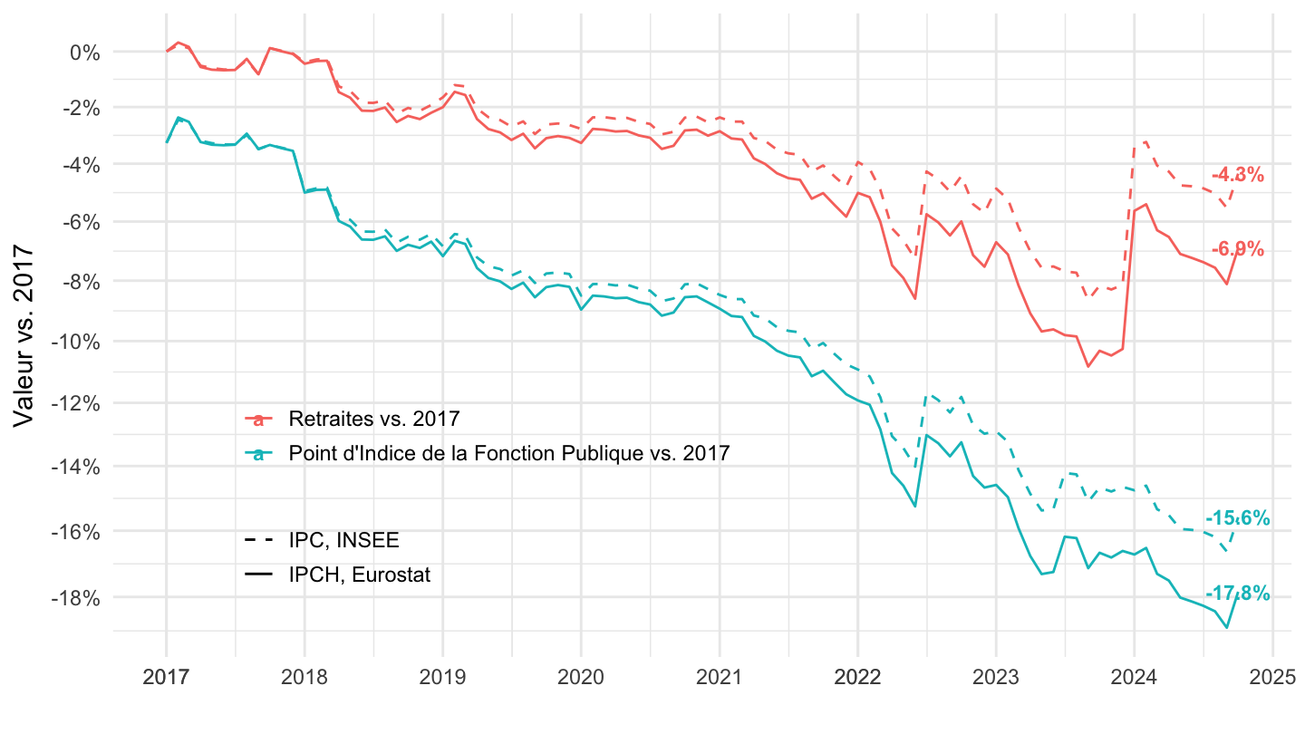

2021-

Retraites

Code

data1 <- revalorisation_pension |>
  select(date, index) |>
  gather(variable, value, -date) |>
  group_by(variable) |>
  complete(date = seq.Date(min(date), max(date), by = "day")) |>
  fill(value) |>
  filter(date >= as.Date("2021-01-01")) |>
  ungroup() |>
  left_join(cpi2_m, by = "date") |>
  filter(day(date) == 1) |>
  filter(date >= as.Date("2021-01-01")) |>
  transmute(date,
            `IPCH, Eurostat` = (value/value[1])*(cpih[1]/cpih),
            `IPC, INSEE` = (value/value[1])*(cpi[1]/cpi)) |>
  gather(type, OBS_VALUE, -date) |>
  mutate(variable = "Retraites vs. 2021")

data1 |>
  ggplot() + geom_line(aes(x = date, y = OBS_VALUE, linetype = type)) + theme_minimal() +
  scale_x_date(breaks = seq(1999, 2100, 1) |> paste0("-01-01") |> as.Date(),
               labels = date_format("%Y")) +
  theme(legend.position = c(0.43, 0.12),
        legend.title = element_blank()) +
  scale_y_log10(breaks = seq(1, 0.02, -0.02),
                labels = percent(seq(1, 0.02, -0.02)-1, acc = 1)) + 
  ylab("Retraites vs. 2021") + xlab("") +
  geom_text(data = . %>% filter(date == max(date)),
            aes(x = date, y = OBS_VALUE, label = percent(OBS_VALUE-1, acc = 0.1)), 
                  fontface ="bold", color = "black", size = 3)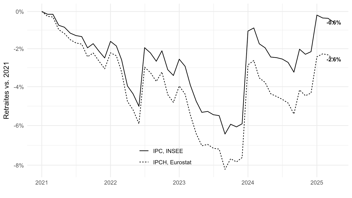

Indice Fonction Publique

Code

net_brut_mensuel <- read_parquet(here::here("data", "insee", "INDICE-TRAITEMENT-FP-net-brut-mensuel.parquet"))
data2 <- indicefp |>
  select(date, point_indice_en_euros) |>
  arrange(desc(date)) |>
  gather(variable, value, -date) |>
  group_by(variable) |>
  complete(date = seq.Date(min(date), max(date), by = "day")) |>
  fill(value) |>
  ungroup() |>
  left_join(cpi2_m, by = "date") |>
  filter(day(date) == 1) |>
  left_join(net_brut_mensuel, by = "date") |>
  filter(date >= as.Date("2021-01-01")) |>
  transmute(date,
            `IPCH, Eurostat` = (value/value[1])*(cpih[1]/cpih)*(net_brut/net_brut[1]),
            `IPC, INSEE` = (value/value[1])*(cpi[1]/cpi)*(net_brut/net_brut[1])) |>
  gather(type, OBS_VALUE, -date) |>
  mutate(variable = "Point d'Indice de la Fonction Publique vs. 2021")

data2 |>
  ggplot() + geom_line(aes(x = date, y = OBS_VALUE, linetype = type)) + theme_minimal() +
  scale_x_date(breaks = c(seq(1999, 2100, 5), seq(1997, 2100, 5)) |> paste0("-01-01") |> as.Date(),
               labels = date_format("%Y")) +
  theme(legend.position = c(0.43, 0.12),
        legend.title = element_blank()) +
  scale_y_log10(breaks = seq(1, 0.02, -0.02),
                labels = percent(seq(1, 0.02, -0.02)-1, acc = 1)) + 
  ylab("Point Indice Fonction Publique vs. 2021") + xlab("") +
  geom_text(data = . %>% filter(date == max(date)),
            aes(x = date, y = OBS_VALUE, label = percent(OBS_VALUE-1, acc = 0.1)), 
                  fontface ="bold", color = "black", size = 3)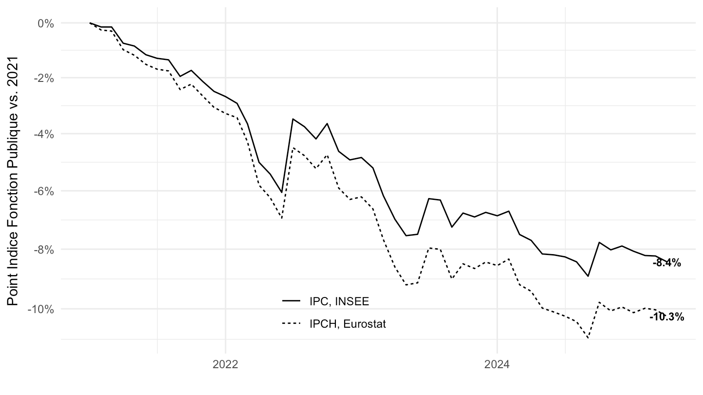

Merge

Code

data2 |>
  bind_rows(data1) |>
  mutate(variable = factor(variable, levels = c("Retraites vs. 2021",
                                                "Point d'Indice de la Fonction Publique vs. 2021"))) |>
  ggplot() + geom_line(aes(x = date, y = OBS_VALUE,  color = variable, linetype = type)) + theme_minimal() +
  scale_linetype_manual(values = c("dashed", "solid")) +
  scale_x_date(breaks = c(seq(1999, 2100, 1), seq(1997, 2100, 5)) |> paste0("-01-01") |> as.Date(),
               labels = date_format("%Y")) +
  theme(legend.position = c(0.32, 0.25),
        legend.title = element_blank(),
        legend.key.size = unit(0.5, "cm")) +
  scale_y_log10(breaks = seq(1, 0.02, -0.02),
                labels = percent(seq(1, 0.02, -0.02)-1, acc = 1)) + 
  ylab("Valeur vs. 2021") + xlab("") +
  geom_label(data = . %>% filter(date == max(date)),
            aes(x = date, y = OBS_VALUE, label = percent(OBS_VALUE-1, acc = 0.1), color = variable), 
                  fontface ="bold",  size = 3, show.legend = F)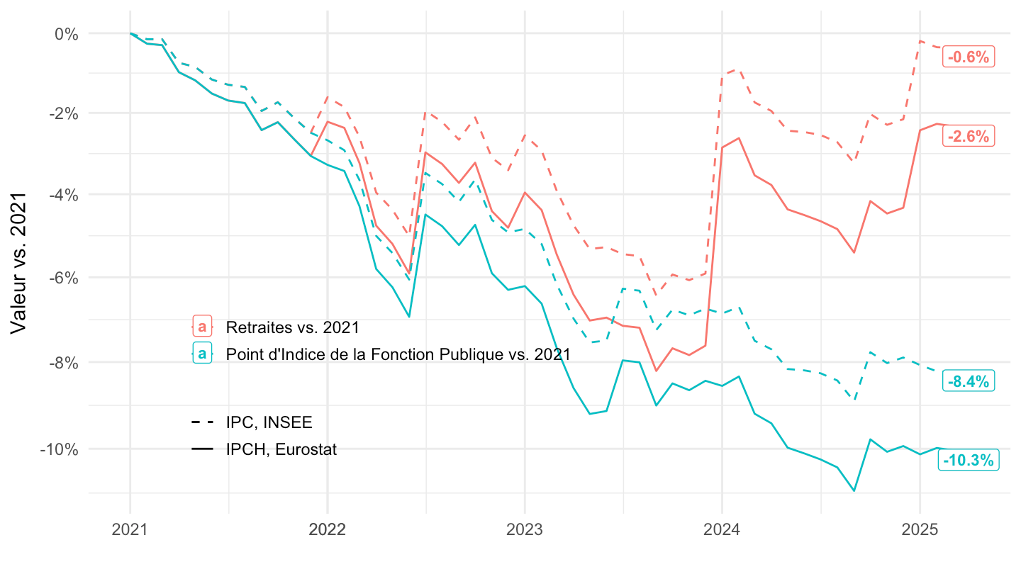

Juin 2017

Retraites

Code

data1 <- revalorisation_pension |>
  select(date, index) |>
  gather(variable, value, -date) |>
  group_by(variable) |>
  complete(date = seq.Date(min(date), max(date), by = "day")) |>
  fill(value) |>
  filter(date >= as.Date("2017-06-01")) |>
  ungroup() |>
  left_join(cpi2_m, by = "date") |>
  filter(day(date) == 1) |>
  filter(date >= as.Date("2017-06-01")) |>
  transmute(date,
            `IPCH, Eurostat` = (value/value[1])*(cpih[1]/cpih),
            `IPC, INSEE` = (value/value[1])*(cpi[1]/cpi)) |>
  gather(type, OBS_VALUE, -date) |>
  mutate(variable = "Retraites vs. juin 2017")

data1 |>
  ggplot() + geom_line(aes(x = date, y = OBS_VALUE, linetype = type)) + theme_minimal() +
  scale_x_date(breaks = seq(1999, 2100, 1) |> paste0("-01-01") |> as.Date(),
               labels = date_format("%Y")) +
  theme(legend.position = c(0.43, 0.12),
        legend.title = element_blank()) +
  scale_y_log10(breaks = seq(1, 0.02, -0.02),
                labels = percent(seq(1, 0.02, -0.02)-1, acc = 1)) + 
  ylab("Retraites vs. juin 2017") + xlab("") +
  geom_text(data = . %>% filter(year(date) %in% seq(1999, 2040, 5),
                                month(date) == 1),
            aes(x = date, y = OBS_VALUE, label = percent(OBS_VALUE-1, acc = 0.1)), 
                  fontface ="bold", color = "black", size = 3)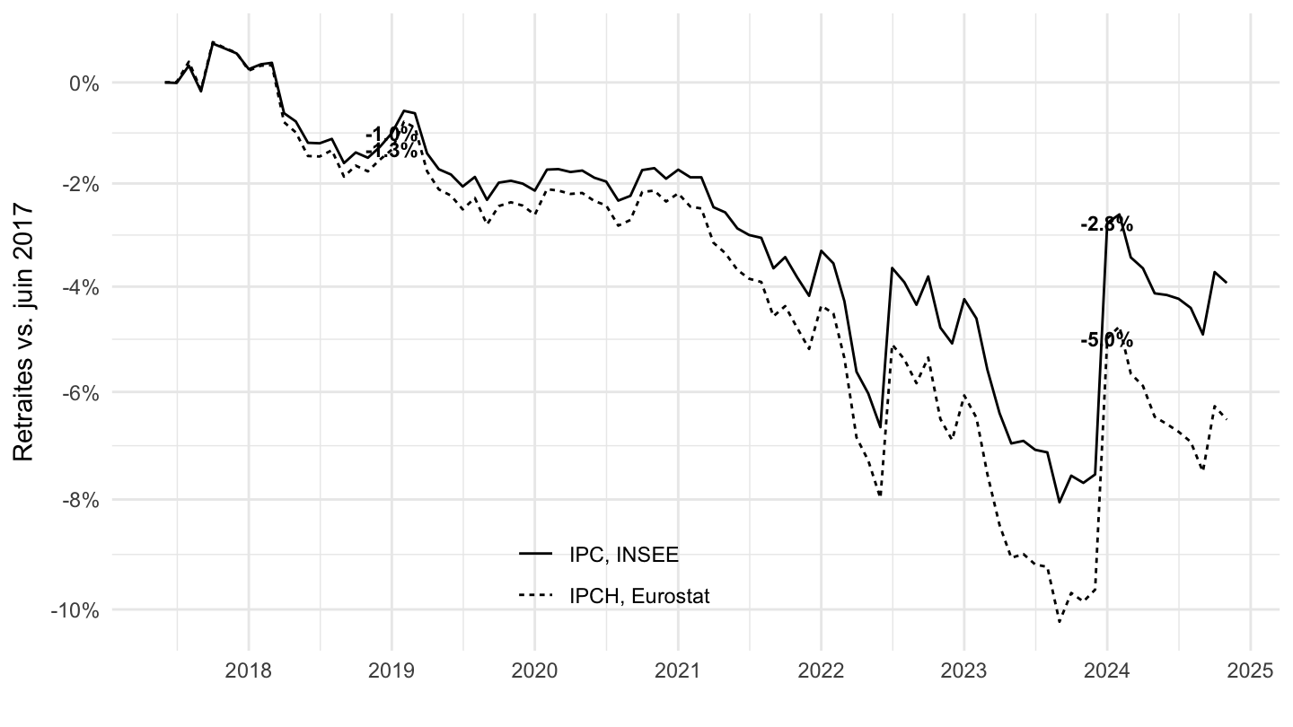

Indice Fonction Publique

Code

net_brut_mensuel <- read_parquet(here::here("data", "insee", "INDICE-TRAITEMENT-FP-net-brut-mensuel.parquet"))
data2 <- indicefp |>
  select(date, point_indice_en_euros) |>
  arrange(desc(date)) |>
  gather(variable, value, -date) |>
  group_by(variable) |>
  complete(date = seq.Date(min(date), max(date), by = "day")) |>
  fill(value) |>
  ungroup() |>
  left_join(cpi2_m, by = "date") |>
  filter(day(date) == 1) |>
  left_join(net_brut_mensuel, by = "date") |>
  filter(date >= as.Date("2017-06-01")) |>
  transmute(date,
            `IPCH, Eurostat` = (value/value[1])*(cpih[1]/cpih)*(net_brut/net_brut[1]),
            `IPC, INSEE` = (value/value[1])*(cpi[1]/cpi)*(net_brut/net_brut[1])) |>
  gather(type, OBS_VALUE, -date) |>
  mutate(variable = "Point d'Indice de la Fonction Publique vs. juin 2017")

data2 |>
  ggplot() + geom_line(aes(x = date, y = OBS_VALUE, linetype = type)) + theme_minimal() +
  scale_x_date(breaks = c(seq(1999, 2100, 5), seq(1997, 2100, 5)) |> paste0("-01-01") |> as.Date(),
               labels = date_format("%Y")) +
  theme(legend.position = c(0.43, 0.12),
        legend.title = element_blank()) +
  scale_y_log10(breaks = seq(1, 0.02, -0.02),
                labels = percent(seq(1, 0.02, -0.02)-1, acc = 1)) + 
  ylab("Point Indice Fonction Publique vs. juin 2017") + xlab("") +
  geom_text(data = . %>% filter(year(date) %in% seq(1999, 2040, 5),
                                month(date) == 1),
            aes(x = date, y = OBS_VALUE, label = percent(OBS_VALUE-1, acc = 0.1)), 
                  fontface ="bold", color = "black", size = 3)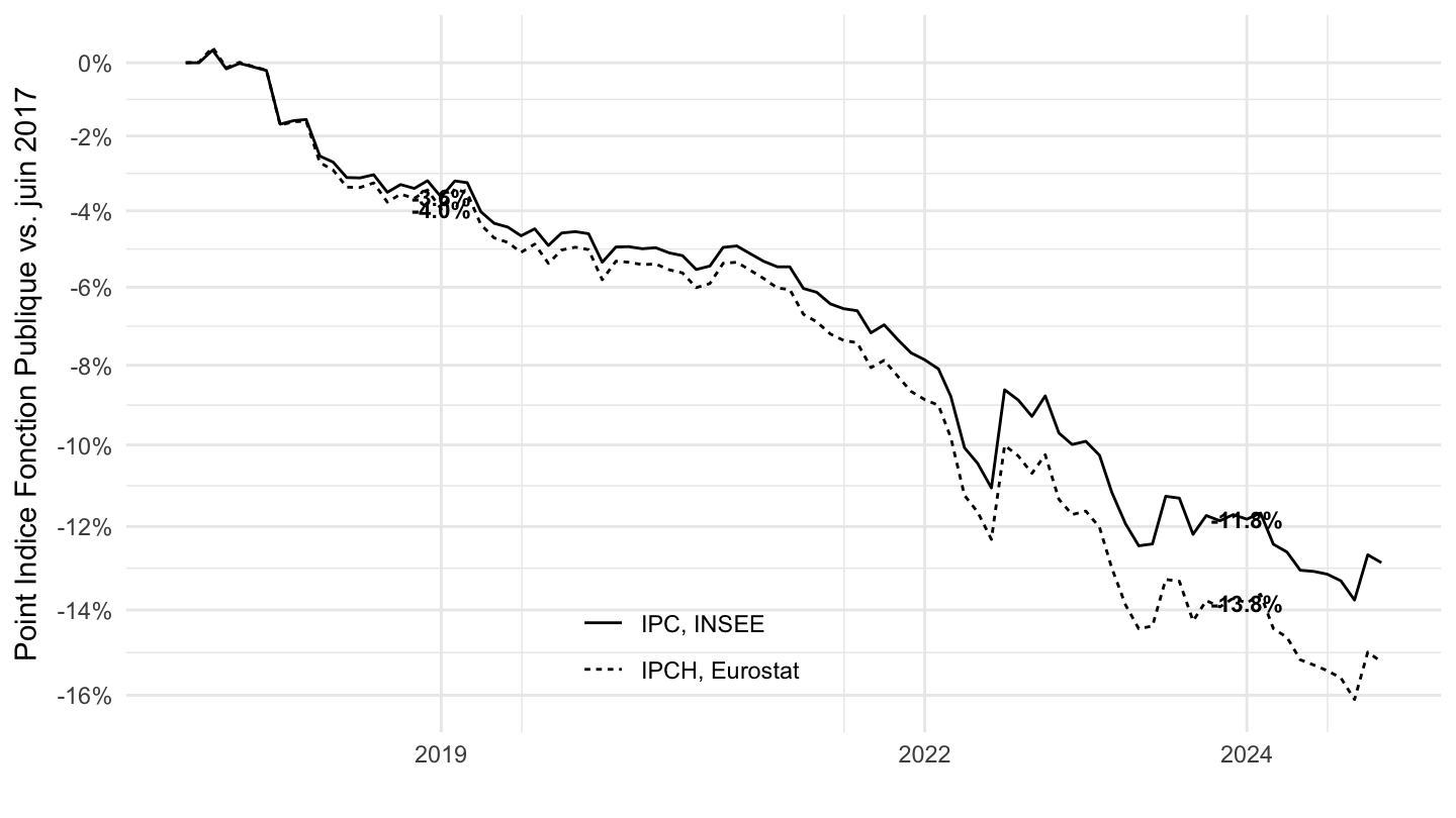

Merge

Code

data2 |>
  bind_rows(data1) |>
  mutate(variable = factor(variable, levels = c("Retraites vs. juin 2017",
                                                "Point d'Indice de la Fonction Publique vs. juin 2017"))) |>
  ggplot() + geom_line(aes(x = date, y = OBS_VALUE,  color = variable, linetype = type)) + theme_minimal() +
  scale_linetype_manual(values = c("dashed", "solid")) +
  scale_x_date(breaks = c(seq(1999, 2100, 1), seq(1997, 2100, 5)) |> paste0("-01-01") |> as.Date(),
               labels = date_format("%Y")) +
  theme(legend.position = c(0.32, 0.25),
        legend.title = element_blank(),
        legend.key.size = unit(0.5, "cm")) +
  scale_y_log10(breaks = seq(1, 0.02, -0.02),
                labels = percent(seq(1, 0.02, -0.02)-1, acc = 1)) + 
  ylab("Valeur vs. 2017") + xlab("") +
  geom_label(data = . %>% filter(date == max(date)),
            aes(x = date, y = OBS_VALUE, label = percent(OBS_VALUE-1, acc = 0.1), color = variable), 
                  fontface ="bold",  size = 3, show.legend = F)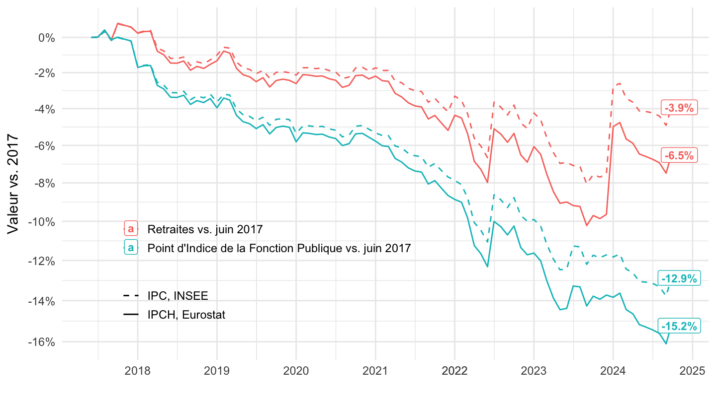

Related Data

Données sur la retraite par capitalisation

source	dataset	Title	Updated
insee	SALAIRES-ANNUELS	Salaires annuels - SALAIRES-ANNUELS	2026-09-12
insee	T_7301	7.301 - Compte des administrations publiques (S13) - T_7301	2026-09-08
ipp	revalorisation_pension	Revalorisation du Régime général de la caisse nationale d’assurance vieillesse (CNAV) - revalorisation_pension	2026-09-12
yahoo	SP500	S&P 500 - SP500	2026-09-12
yahoo	indices	Indices - indices	2026-09-12

Données sur l’évolution du pouvoir d’achat

source	dataset	Title	Updated
eurostat	nasq_10_nf_tr	Non-financial transactions - nasq_10_nf_tr	2026-09-09
insee	CNA-2014-RDB	Revenu et pouvoir d’achat des ménages - CNA-2014-RDB	2026-09-12
insee	SALAIRES-ANNUELS	Salaires annuels - SALAIRES-ANNUELS	2026-09-12
insee	T_7401	7.401 – Compte des ménages (S14) (En milliards d’euros) - T_7401	2026-09-08
insee	econ-gen-revenu-dispo-pouv-achat-2	Revenu disponible brut et pouvoir d’achat - Données annuelles - econ-gen-revenu-dispo-pouv-achat-2	2026-08-02
insee	reve-niv-vie-individu-activite	Niveau de vie selon l’activité - Données annuelles - reve-niv-vie-individu-activite	2026-08-02
insee	t_men_val	Revenu, pouvoir d’achat et comptes des ménages - Valeurs aux prix courants - t_men_val	2026-09-03
insee	t_pib_vol	PIB et ses composantes - Equilibre emplois-ressources - volumes aux prix de l’année précédente chaînés - t_pib_vol	2026-09-03
insee	t_pouvachat_val	Pouvoir d’achat et ratios des comptes des ménages - t_pouvachat_val	2026-09-03
insee	t_recapAgent_val	Récapitulatif des séries des comptes d’agents - t_recapAgent_val	2026-09-03
ipp	indicefp	Point d’indice de la fonction publique - indicefp	2026-09-12
ipp	revalorisation_pension	Revalorisation du Régime général de la caisse nationale d’assurance vieillesse (CNAV) - revalorisation_pension	2026-09-12
oecd	NAAG	National Accounts at a Glance - NAAG	2026-08-02
oecd	PRICES_CPI	Consumer price indices (CPIs) - PRICES_CPI	2026-08-02

Évolution du pouvoir d’achat depuis 2017

source	dataset	Title	Updated
dares	les-indices-de-salaire-de-base	Les indices de salaire de base - les-indices-de-salaire-de-base	2026-08-30
eurostat	nama_10_pc	Main GDP aggregates per capita - nama_10_pc	2026-09-09
eurostat	nasq_10_nf_tr	Non-financial transactions - nasq_10_nf_tr	2026-09-09
insee	CNA-2020-CONSO-MEN	Consommation des ménages - CNA-2020-CONSO-MEN	2026-09-04
insee	INDICES_LOYERS	Indices des loyers d’habitation (ILH) - INDICES_LOYERS	2026-09-12
insee	IPEA-2021	Indice des prix d’entretien-amélioration des bâtiments - Base 2021 - IPEA-2021	2026-09-12
insee	IRL	Indice pour la révision d’un loyer d’habitation - IRL	2026-09-12
insee	SALAIRES-ANNUELS	Salaires annuels - SALAIRES-ANNUELS	2026-09-12
insee	SMIC-COTISATIONS	Taux de cotisations et salaires minima garantis - SMIC-COTISATIONS	2026-09-12
insee	T_2101	2.101 – Revenu disponible brut des ménages et évolution du pouvoir d’achat par personne, par ménage et par unité de consommation (En milliards euros et %) - t_2101	2026-09-13
insee	T_2103	2.103 – Dépense de consommation finale pré-engagée des ménages à prix courants (En milliards d’euros et %) - t_2103	2026-09-13
insee	T_7401	7.401 – Compte des ménages (S14) (En milliards d’euros) - T_7401	2026-09-08
insee	econ-gen-revenu-dispo-pouv-achat-2	Revenu disponible brut et pouvoir d’achat - Données annuelles - econ-gen-revenu-dispo-pouv-achat-2	2026-08-02
insee	t_men_val	Revenu, pouvoir d’achat et comptes des ménages - Valeurs aux prix courants - t_men_val	2026-09-03
insee	t_pib_vol	PIB et ses composantes - Equilibre emplois-ressources - volumes aux prix de l’année précédente chaînés - t_pib_vol	2026-09-03
insee	t_pouvachat_val	Pouvoir d’achat et ratios des comptes des ménages - t_pouvachat_val	2026-09-03
insee	t_recapAgent_val	Récapitulatif des séries des comptes d’agents - t_recapAgent_val	2026-09-03
insee	t_salaire_val	Salaire moyen par tête - SMPT (données CVS) - t_salaire_val	2026-09-03
ipp	indicefp	Point d’indice de la fonction publique - indicefp	2026-09-12
ipp	revalorisation_pension	Revalorisation du Régime général de la caisse nationale d’assurance vieillesse (CNAV) - revalorisation_pension	2026-09-12
oecd	PRICES_ALL	Consumer price indices (CPIs) - PRICES_ALL	2026-09-11

Statistiques sur les retraites

source	dataset	Title	Updated
insee	DECES-MORTALITE	Décès et mortalité - DECES-MORTALITE	2026-09-12
insee	T_3301	3.301 – Dépenses des administrations publiques (S13) ventilées par fonction (En milliards d’euros) - T_3301	2026-09-09
ipp	revalorisation_pension	Revalorisation du Régime général de la caisse nationale d’assurance vieillesse (CNAV) - revalorisation_pension	2026-09-12