Indice de traitement brut dans la fonction publique de l’État
Données - INSEE
Info
Last observation: 2026-Q1
First observation: 2000-Q4
Number of observations: 816
Last data update: 26 jul 2026, 02:05. Last compile: 26 jul 2026, 05:12
Structure
Données sur les salaires
| source | dataset | Title | .html | .rData |
|---|---|---|---|---|
| insee | INDICE-TRAITEMENT-FP | Indice de traitement brut dans la fonction publique de l'État | 2026-07-24 | 2026-07-23 |
| dares | les-indices-de-salaire-de-base | Les indices de salaire de base | 2026-07-20 | 2026-05-21 |
| insee | CNA-2014-RDB | Revenu et pouvoir d’achat des ménages | 2026-07-24 | 2026-07-24 |
| insee | CNT-2014-CSI | Comptes de secteurs institutionnels | 2026-07-24 | 2026-07-24 |
| insee | ECRT2023 | Emploi, chômage, revenus du travail - Edition 2023 | 2026-07-24 | 2023-06-30 |
| insee | SALAIRES-ACEMO | Indices trimestriels de salaires dans le secteur privé - Résultats par secteur d’activité | 2026-07-24 | 2026-07-24 |
| insee | SALAIRES-ACEMO-2017 | Indices trimestriels de salaires dans le secteur privé | 2026-07-24 | 2026-07-24 |
| insee | SALAIRES-ANNUELS | Salaires annuels | 2026-07-24 | 2026-07-24 |
| insee | T_2101 | 2.101 – Revenu disponible brut des ménages et évolution du pouvoir d'achat par personne, par ménage et par unité de consommation (En milliards euros et %) | 2026-07-24 | 2025-12-14 |
| insee | T_7401 | 7.401 – Compte des ménages (S14) (En milliards d'euros) | 2026-07-24 | 2025-12-14 |
| insee | if230 | Séries longues sur les salaires dans le secteur privé | 2026-07-24 | 2021-12-04 |
| insee | ir_salaires_SL_23_csv | NA | NA | NA |
| insee | ir_salaires_SL_csv | NA | NA | NA |
| insee | t_salaire_val | Salaire moyen par tête - SMPT (données CVS) | 2026-07-24 | 2026-02-27 |
LAST_COMPILE
| LAST_COMPILE |
|---|
| 2026-07-26 |
Last
Code
`INDICE-TRAITEMENT-FP` %>%
  group_by(TIME_PERIOD) %>%
  summarise(Nobs = n()) %>%
  arrange(desc(TIME_PERIOD)) %>%
  head(2) %>%
print_table_conditional()| TIME_PERIOD | Nobs |
|---|---|
| 2026-Q1 | 8 |
| 2025-Q4 | 8 |
Par type
Net et Brut
Code
`INDICE-TRAITEMENT-FP` %>%
  #filter(CATEGORIE_FP == "A") %>%


  quarter_to_date %>%
  ggplot() + geom_line(aes(x = date, y = OBS_VALUE,  linetype = Indicateur, color = Categorie_fp)) +
  theme_minimal() + ylab("Indice") + xlab("") +
  scale_x_date(breaks = seq(1920, 2100, 2) %>% paste0("-01-01") %>% as.Date,
               labels = date_format("%Y")) +
  theme(legend.position = c(0.3, 0.7),
        legend.title = element_blank()) +
  scale_y_log10(breaks = seq(0, 200, 2))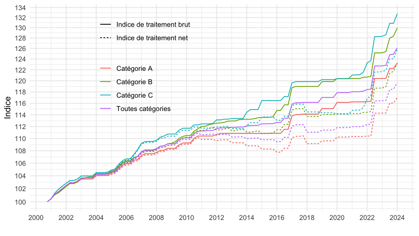
Net
Code
`INDICE-TRAITEMENT-FP` %>%
  filter(INDICATEUR == "NSALNF") %>%


  quarter_to_date %>%
  arrange(date) %>%
  ggplot() + geom_line(aes(x = date, y = OBS_VALUE,  color = Categorie_fp)) +
  theme_minimal() + ylab("Indice Net") + xlab("") +
  scale_x_date(breaks = seq(1920, 2100, 2) %>% paste0("-01-01") %>% as.Date,
               labels = date_format("%Y")) +
  theme(legend.position = c(0.3, 0.7),
        legend.title = element_blank()) +
  scale_y_log10(breaks = seq(0, 200, 1))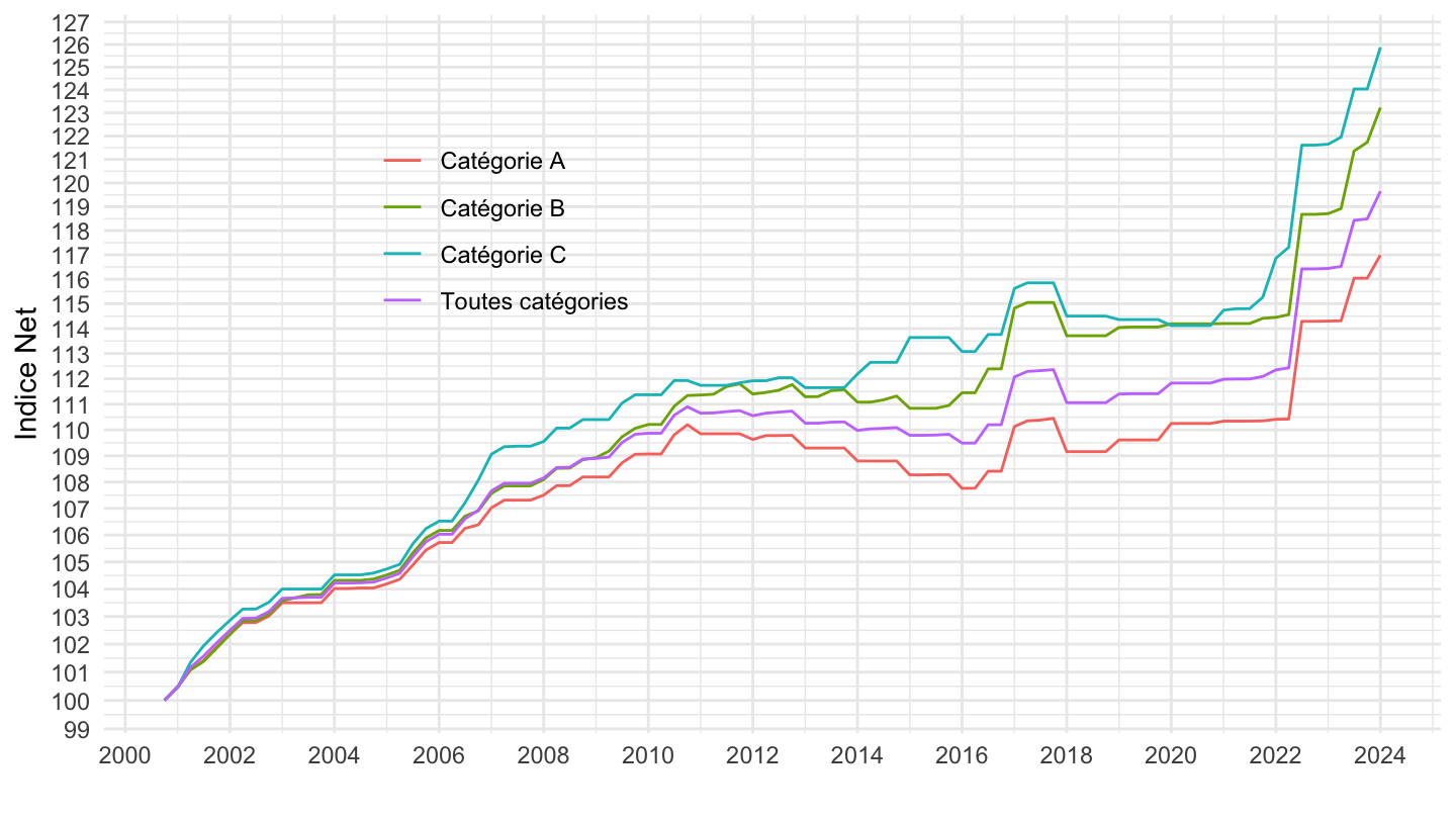
Brut
Code
`INDICE-TRAITEMENT-FP` %>%
  filter(INDICATEUR == "NSALBF") %>%


  quarter_to_date %>%
  ggplot() + geom_line(aes(x = date, y = OBS_VALUE,  color = Categorie_fp)) +
  theme_minimal() + ylab("Indice Brut") + xlab("") +
  scale_x_date(breaks = seq(1920, 2100, 2) %>% paste0("-01-01") %>% as.Date,
               labels = date_format("%Y")) +
  theme(legend.position = c(0.3, 0.7),
        legend.title = element_blank()) +
  scale_y_log10(breaks = seq(0, 200, 2))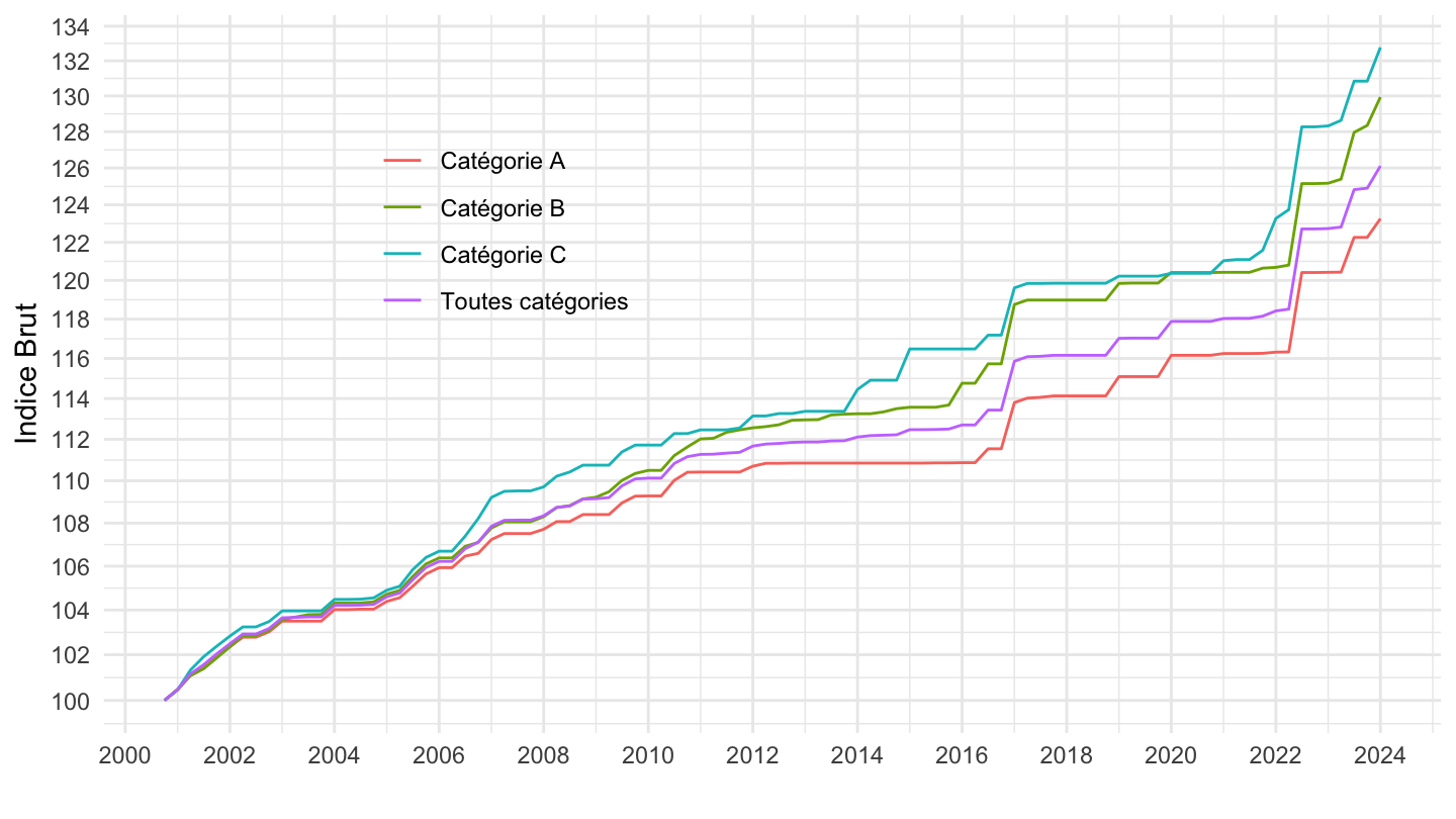
Indice de traitement brut dans la fonction publique de l’État
Tous
Nominal
Code
`INDICE-TRAITEMENT-FP` %>%
  filter(CATEGORIE_FP == "T") %>%

  quarter_to_date %>%
  ggplot() + geom_line(aes(x = date, y = OBS_VALUE,  color = Indicateur)) +
  theme_minimal() + ylab("Indice, Tous") + xlab("") +
  scale_x_date(breaks = seq(1920, 2100, 2) %>% paste0("-01-01") %>% as.Date,
               labels = date_format("%Y")) +
  theme(legend.position = c(0.7, 0.2),
        legend.title = element_blank()) +

  scale_y_log10(breaks = seq(0, 200, 1))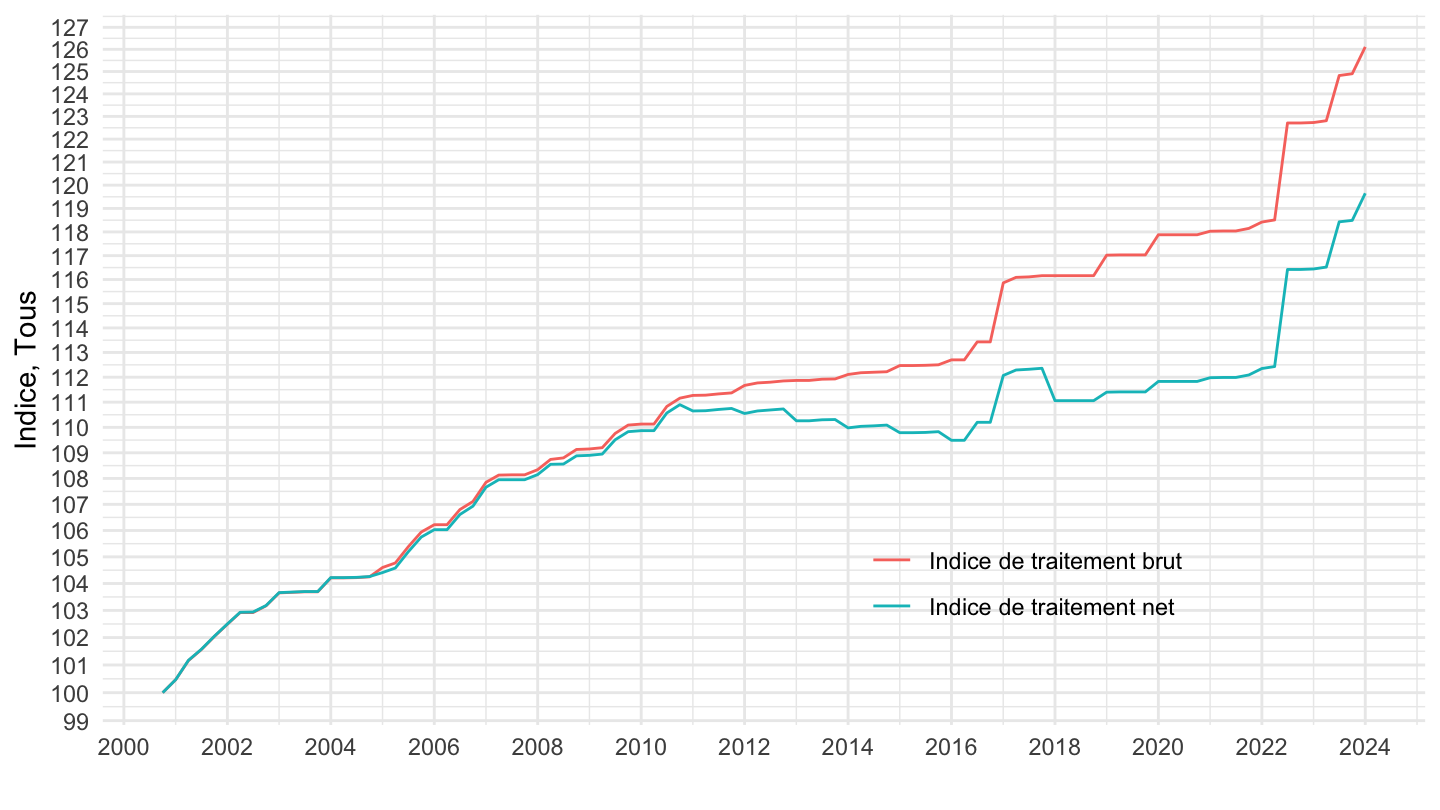
Indice Net
Code
`INDICE-TRAITEMENT-FP` %>%
  filter(CATEGORIE_FP == "T",
         INDICATEUR == "NSALNF") %>%

  quarter_to_date %>%
  left_join(inflation, by = "date") %>%
  arrange(date) %>%
  transmute(date, `Indice de traitement net, nominal` = OBS_VALUE,
            `Indice de traitement net, réel` = IPCH[1]*OBS_VALUE/IPCH) %>%
  gather(variable, value, -date) %>%
  ggplot() + geom_line(aes(x = date, y = value,  color = variable)) +
  theme_minimal() + ylab("Indice, Tous") + xlab("") +
  scale_x_date(breaks = seq(1920, 2100, 2) %>% paste0("-01-01") %>% as.Date,
               labels = date_format("%Y")) +
  theme(legend.position = c(0.2, 0.2),
        legend.title = element_blank()) +
  scale_y_log10(breaks = seq(0, 200, 5))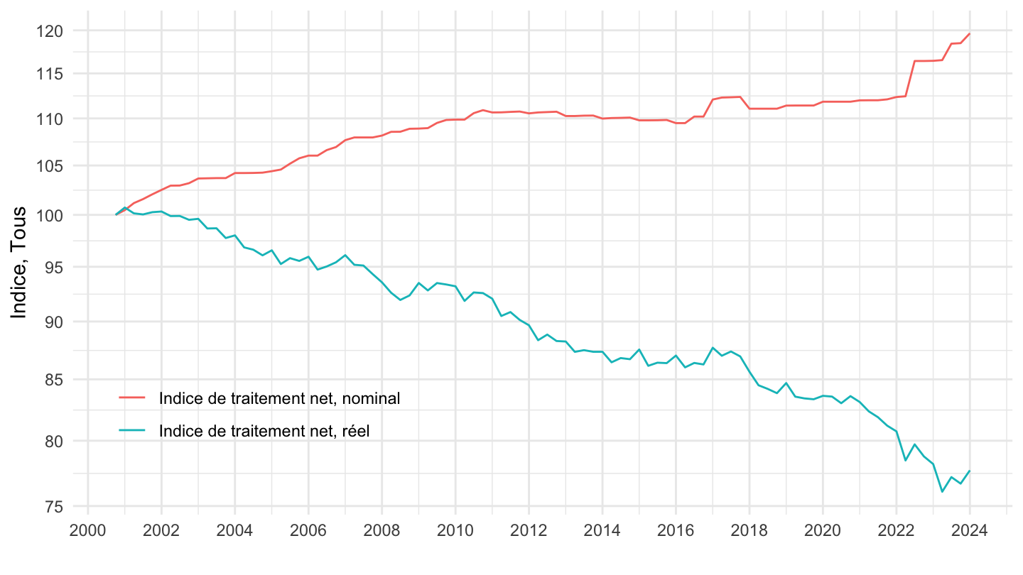
Indice Brut
Code
`INDICE-TRAITEMENT-FP` %>%
  filter(CATEGORIE_FP == "T",
         INDICATEUR == "NSALBF") %>%

  quarter_to_date %>%
  left_join(inflation, by = "date") %>%
  arrange(date) %>%
  transmute(date, `Indice de traitement brut, nominal` = OBS_VALUE,
            `Indice de traitement brut, réel` = IPCH[1]*OBS_VALUE/IPCH) %>%
  gather(variable, value, -date) %>%
  ggplot() + geom_line(aes(x = date, y = value,  color = variable)) +
  theme_minimal() + ylab("Indice, Tous") + xlab("") +
  scale_x_date(breaks = seq(1920, 2100, 2) %>% paste0("-01-01") %>% as.Date,
               labels = date_format("%Y")) +
  theme(legend.position = c(0.2, 0.2),
        legend.title = element_blank()) +
  scale_y_log10(breaks = seq(0, 200, 5))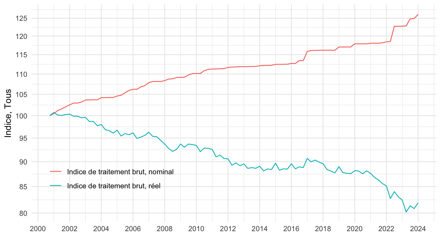
Indice Net/brut
Code
`INDICE-TRAITEMENT-FP` %>%
  filter(CATEGORIE_FP == "A") %>%

  quarter_to_date %>%
  left_join(inflation, by = "date") %>%
  arrange(date) %>%
  transmute(date, Indicateur, `Nominal` = OBS_VALUE,
            `Réel` = IPCH[1]*OBS_VALUE/IPCH) %>%
  gather(variable, value, -date, -Indicateur) %>%
  ggplot() + geom_line(aes(x = date, y = value,  color = variable, linetype = Indicateur)) +
  theme_minimal() + ylab("Indice, Tous") + xlab("") +
  scale_x_date(breaks = seq(1920, 2100, 2) %>% paste0("-01-01") %>% as.Date,
               labels = date_format("%Y")) +
  theme(legend.position = c(0.2, 0.2),
        legend.title = element_blank()) +
  scale_y_log10(breaks = seq(0, 200, 5))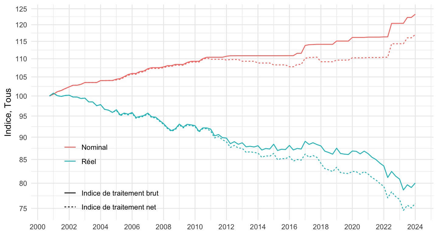
Indice Net/brut, réel IPC IPCH
Code
`INDICE-TRAITEMENT-FP` %>%
  filter(CATEGORIE_FP == "T") %>%

  quarter_to_date %>%
  left_join(inflation, by = "date") %>%
  arrange(date) %>%
  transmute(date, Indicateur,
            `Nominal` = OBS_VALUE,
            `Réel (inflation IPCH)` = IPCH[1]*OBS_VALUE/IPCH,
            `Réel (inflation IPC)` = IPC[1]*OBS_VALUE/IPC) %>%
  gather(variable, value, -date, -Indicateur) %>%
  ggplot() + geom_line(aes(x = date, y = value,  color = variable, linetype = Indicateur)) +
  theme_minimal() + ylab("Indice de traitement dans la fonction publique de l'État") + xlab("") +
  scale_color_manual(values = c("darkgrey", "#F8766D", "#619CFF")) +
  scale_x_date(breaks = seq(1920, 2100, 2) %>% paste0("-01-01") %>% as.Date,
               labels = date_format("%Y")) +
  theme(legend.position = c(0.18, 0.24),
        legend.title = element_blank()) +
  scale_y_log10(breaks = seq(0, 200, 2))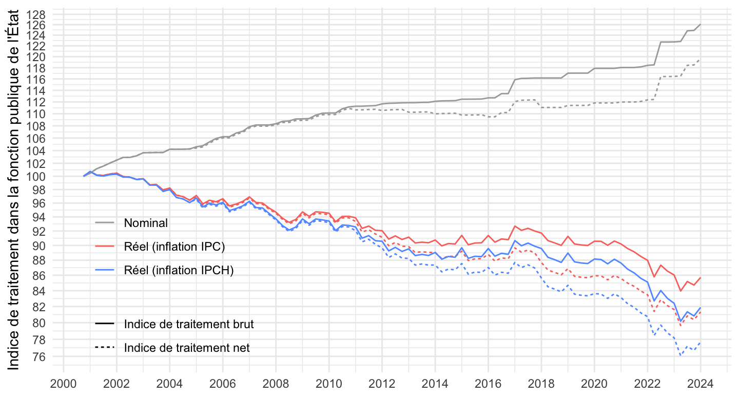
Ratio Net/brut
Annuel
Code
net_brut_annuel <- `INDICE-TRAITEMENT-FP` %>%
  filter(CATEGORIE_FP == "T") %>%

  quarter_to_date %>%
  arrange(date) %>%
  select(date, OBS_VALUE, Indicateur) %>%
  spread(Indicateur, OBS_VALUE) %>%
  transmute(date, net_brut = `Indice de traitement net`/`Indice de traitement brut`) %>%
  filter(month(date) == 1) %>%
  slice(1, 1:n(), n()) %>%
  mutate(date = case_when(row_number() == n() ~ Sys.Date(),
                              row_number() == 1 ~ as.Date("1960-01-01"),
                              TRUE ~ date)) %>%
  complete(date = seq.Date(min(date), max(date), by = "year")) %>%
  fill(net_brut)

save(net_brut_annuel, file = "INDICE-TRAITEMENT-FP-net-brut-annuel.RData")

net_brut_annuel %>%
  ggplot() + geom_line(aes(x = date, y = net_brut-1)) +
  theme_minimal() + ylab("Ratio net/brut") + xlab("") +
  scale_color_manual(values = c("#F8766D", "#619CFF")) +
  scale_x_date(breaks = seq(1920, 2100, 5) %>% paste0("-01-01") %>% as.Date,
               labels = date_format("%Y")) +
  theme(legend.position = c(0.18, 0.24),
        legend.title = element_blank()) +
  scale_y_continuous(breaks = seq(-1,1, 0.01),
                     labels = percent_format(a = 1))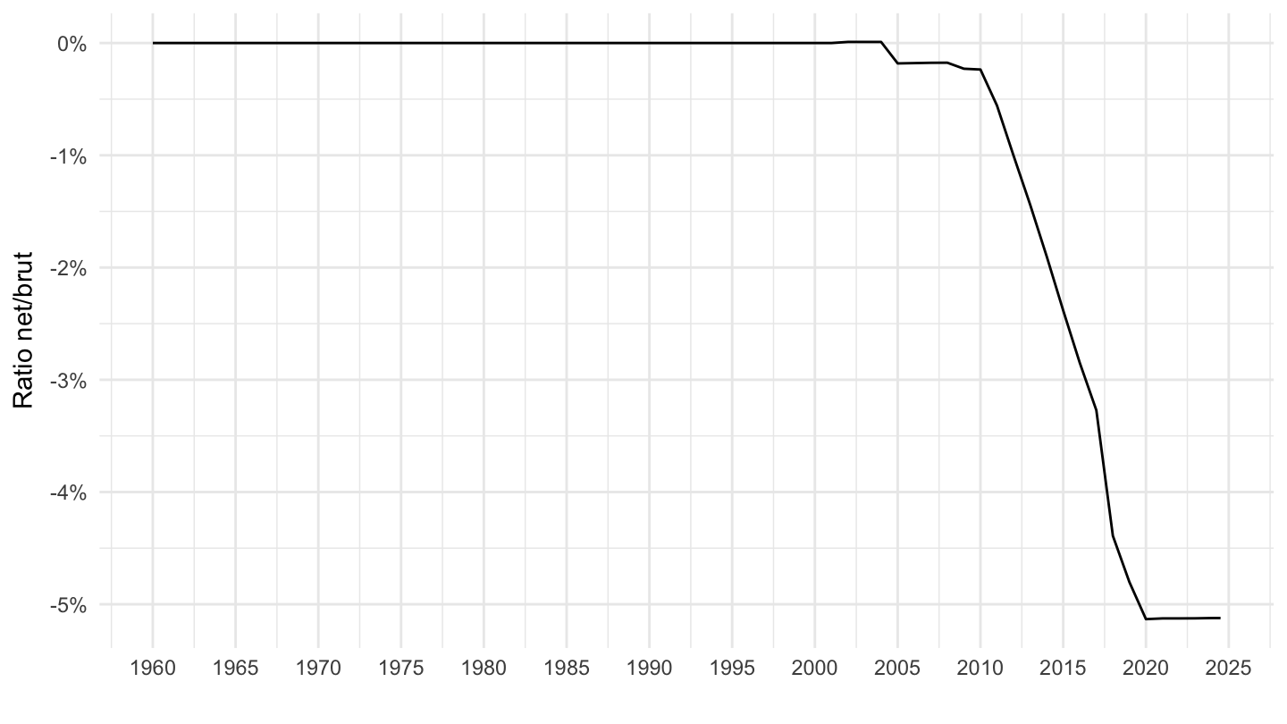
Trimestriel
Code
net_brut_trimestriel <- `INDICE-TRAITEMENT-FP` %>%
  filter(CATEGORIE_FP == "T") %>%

  quarter_to_date %>%
  arrange(date) %>%
  select(date, OBS_VALUE, Indicateur) %>%
  spread(Indicateur, OBS_VALUE) %>%
  transmute(date, net_brut = `Indice de traitement net`/`Indice de traitement brut`) %>%
  slice(1, 1:n(), n()) %>%
  mutate(date = case_when(row_number() == n() ~ Sys.Date(),
                              row_number() == 1 ~ as.Date("1960-01-01"),
                              TRUE ~ date)) %>%
  complete(date = seq.Date(min(date), max(date), by = "quarter")) %>%
  fill(net_brut)

save(net_brut_trimestriel, file = "INDICE-TRAITEMENT-FP-net-brut-trimestriel.RData")

net_brut_trimestriel %>%
  ggplot() + geom_line(aes(x = date, y = net_brut-1)) +
  theme_minimal() + ylab("Ratio net/brut") + xlab("") +
  scale_color_manual(values = c("#F8766D", "#619CFF")) +
  scale_x_date(breaks = seq(1920, 2100, 5) %>% paste0("-01-01") %>% as.Date,
               labels = date_format("%Y")) +
  theme(legend.position = c(0.18, 0.24),
        legend.title = element_blank()) +
  scale_y_continuous(breaks = seq(-1,1, 0.01),
                     labels = percent_format(a = 1))
Mensuel
Code
net_brut_mensuel <- `INDICE-TRAITEMENT-FP` %>%
  filter(CATEGORIE_FP == "T") %>%

  quarter_to_date %>%
  arrange(date) %>%
  select(date, OBS_VALUE, Indicateur) %>%
  spread(Indicateur, OBS_VALUE) %>%
  transmute(date, net_brut = `Indice de traitement net`/`Indice de traitement brut`) %>%
  slice(1, 1:n(), n()) %>%
  mutate(date = case_when(row_number() == n() ~ Sys.Date(),
                              row_number() == 1 ~ as.Date("1960-01-01"),
                              TRUE ~ date)) %>%
  complete(date = seq.Date(min(date), max(date), by = "month")) %>%
  fill(net_brut)

save(net_brut_mensuel, file = "INDICE-TRAITEMENT-FP-net-brut-mensuel.RData")

net_brut_mensuel %>%
  ggplot() + geom_line(aes(x = date, y = net_brut-1)) +
  theme_minimal() + ylab("Ratio net/brut") + xlab("") +
  scale_color_manual(values = c("#F8766D", "#619CFF")) +
  scale_x_date(breaks = seq(1920, 2100, 5) %>% paste0("-01-01") %>% as.Date,
               labels = date_format("%Y")) +
  theme(legend.position = c(0.18, 0.24),
        legend.title = element_blank()) +
  scale_y_continuous(breaks = seq(-1,1, 0.01),
                     labels = percent_format(a = 1))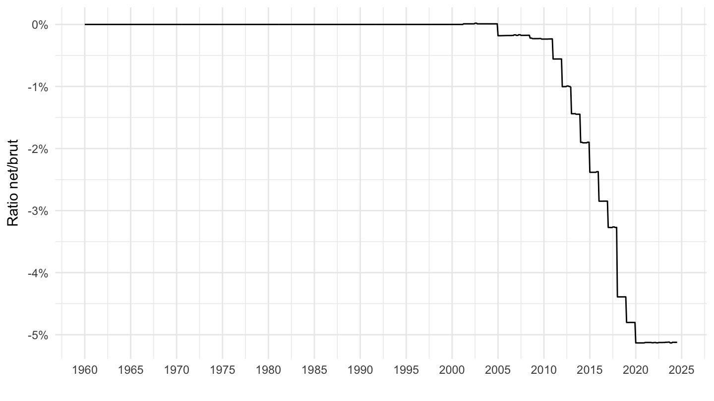
Indice Net/brut, réel IPC IPCH
Code
`INDICE-TRAITEMENT-FP` %>%
  filter(CATEGORIE_FP == "T") %>%

  quarter_to_date %>%
  left_join(inflation, by = "date") %>%
  arrange(date) %>%
  transmute(date, Indicateur,
            `Réel (inflation IPCH)` = IPCH[1]*OBS_VALUE/IPCH,
            `Réel (inflation IPC)` = IPC[1]*OBS_VALUE/IPC) %>%
  gather(variable, value, -date, -Indicateur) %>%
  ggplot() + geom_line(aes(x = date, y = value,  color = variable, linetype = Indicateur)) +
  theme_minimal() + ylab("Indice de traitement dans la FP de l'État") + xlab("") +
  scale_color_manual(values = c("#F8766D", "#619CFF")) +
  scale_x_date(breaks = seq(1921, 2100, 2) %>% paste0("-01-01") %>% as.Date,
               labels = date_format("%Y")) +
  theme(legend.position = c(0.18, 0.24),
        legend.title = element_blank()) +
  scale_y_log10(breaks = seq(0, 200, 2))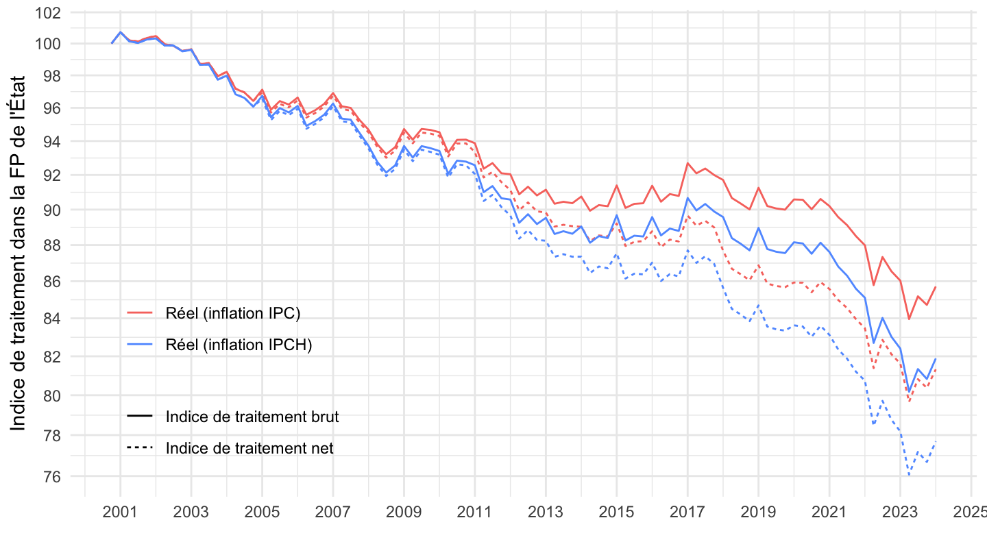
Catégorie A
Nominal
Code
`INDICE-TRAITEMENT-FP` %>%
  filter(CATEGORIE_FP == "A") %>%

  quarter_to_date %>%
  ggplot() + geom_line(aes(x = date, y = OBS_VALUE,  color = Indicateur)) +
  theme_minimal() + ylab("Indice, Catégorie A") + xlab("") +
  scale_x_date(breaks = seq(1920, 2100, 2) %>% paste0("-01-01") %>% as.Date,
               labels = date_format("%Y")) +
  theme(legend.position = c(0.7, 0.2),
        legend.title = element_blank()) +

  scale_y_log10(breaks = seq(0, 200, 1))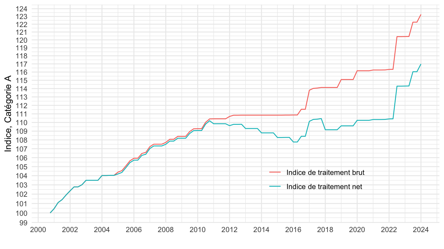
Indice Net
Code
`INDICE-TRAITEMENT-FP` %>%
  filter(CATEGORIE_FP == "A",
         INDICATEUR == "NSALNF") %>%

  quarter_to_date %>%
  left_join(inflation, by = "date") %>%
  arrange(date) %>%
  transmute(date, `Indice de traitement net, nominal` = OBS_VALUE,
            `Indice de traitement net, réel` = IPCH[1]*OBS_VALUE/IPCH) %>%
  gather(variable, value, -date) %>%
  ggplot() + geom_line(aes(x = date, y = value,  color = variable)) +
  theme_minimal() + ylab("Indice, Catégorie A") + xlab("") +
  scale_x_date(breaks = seq(1920, 2100, 2) %>% paste0("-01-01") %>% as.Date,
               labels = date_format("%Y")) +
  theme(legend.position = c(0.2, 0.2),
        legend.title = element_blank()) +
  scale_y_log10(breaks = seq(0, 200, 5))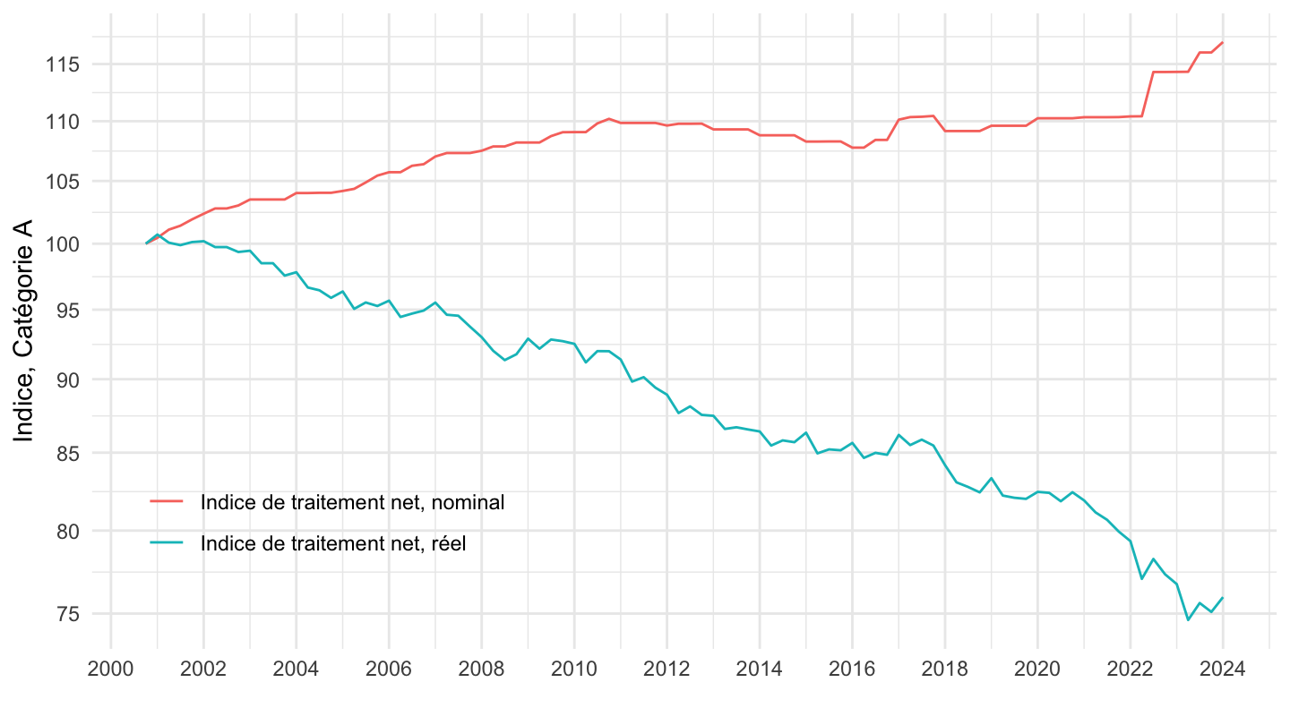
Indice Brut
Code
`INDICE-TRAITEMENT-FP` %>%
  filter(CATEGORIE_FP == "A",
         INDICATEUR == "NSALBF") %>%

  quarter_to_date %>%
  left_join(inflation, by = "date") %>%
  arrange(date) %>%
  transmute(date, `Indice de traitement brut, nominal` = OBS_VALUE,
            `Indice de traitement brut, réel` = IPCH[1]*OBS_VALUE/IPCH) %>%
  gather(variable, value, -date) %>%
  ggplot() + geom_line(aes(x = date, y = value,  color = variable)) +
  theme_minimal() + ylab("Indice, Catégorie A") + xlab("") +
  scale_x_date(breaks = seq(1920, 2100, 2) %>% paste0("-01-01") %>% as.Date,
               labels = date_format("%Y")) +
  theme(legend.position = c(0.2, 0.2),
        legend.title = element_blank()) +
  scale_y_log10(breaks = seq(0, 200, 5))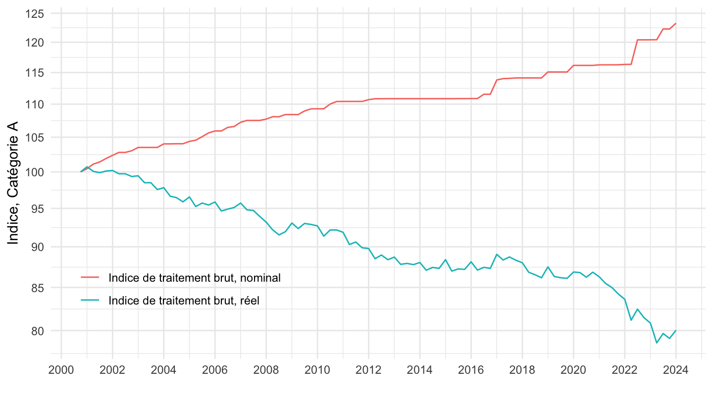
Indice Net/brut
Code
`INDICE-TRAITEMENT-FP` %>%
  filter(CATEGORIE_FP == "A") %>%

  quarter_to_date %>%
  left_join(inflation, by = "date") %>%
  arrange(date) %>%
  transmute(date, Indicateur, `Nominal` = OBS_VALUE,
            `Réel` = IPCH[1]*OBS_VALUE/IPCH) %>%
  gather(variable, value, -date, -Indicateur) %>%
  ggplot() + geom_line(aes(x = date, y = value,  color = variable, linetype = Indicateur)) +
  theme_minimal() + ylab("Indice, Catégorie A") + xlab("") +
  scale_x_date(breaks = seq(1920, 2100, 2) %>% paste0("-01-01") %>% as.Date,
               labels = date_format("%Y")) +
  theme(legend.position = c(0.2, 0.2),
        legend.title = element_blank()) +
  scale_y_log10(breaks = seq(0, 200, 5))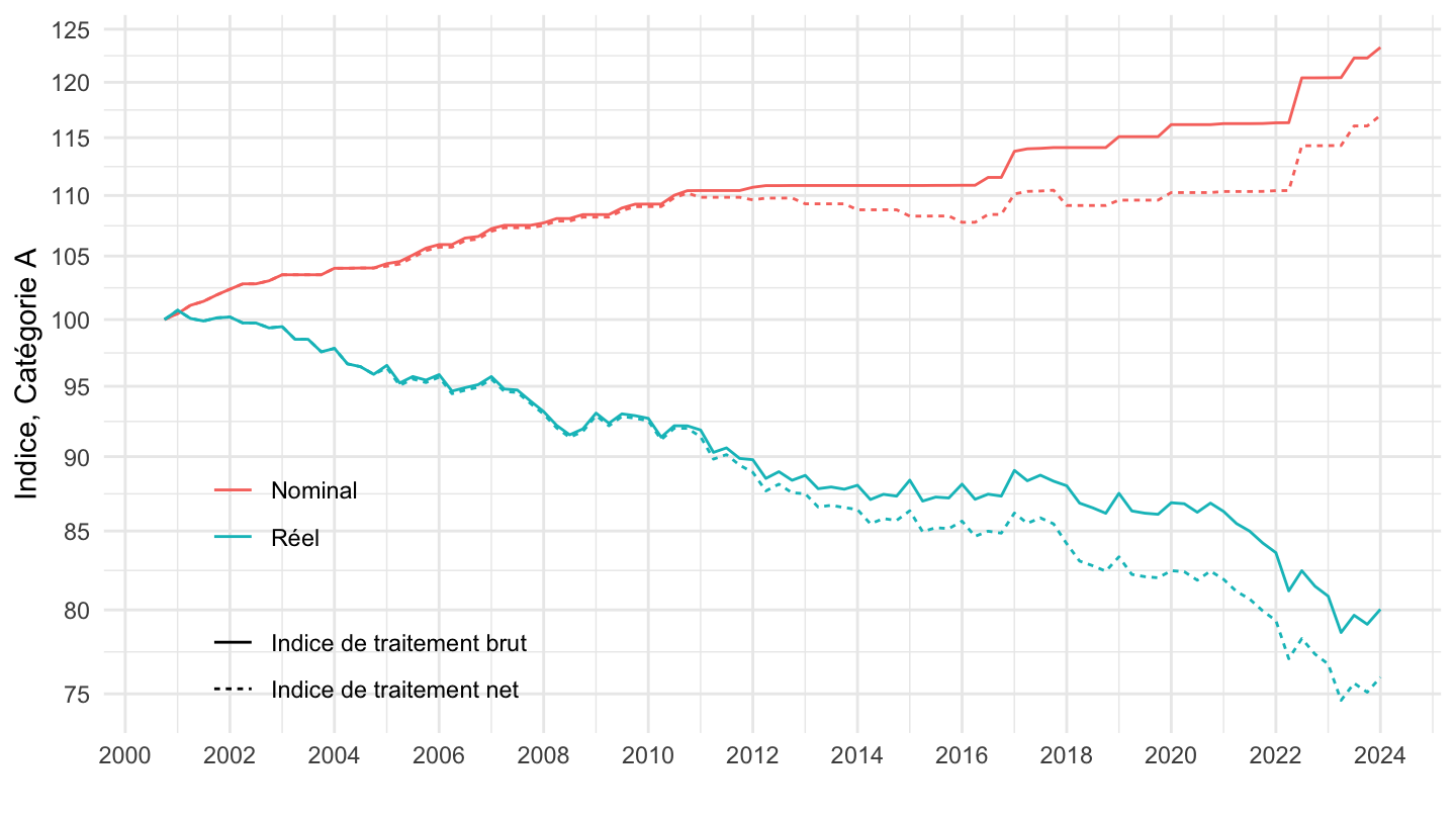
Indice Net/brut, réel IPC IPCH
Code
`INDICE-TRAITEMENT-FP` %>%
  filter(CATEGORIE_FP == "A") %>%

  quarter_to_date %>%
  left_join(inflation, by = "date") %>%
  arrange(date) %>%
  transmute(date, Indicateur,
            `Nominal` = OBS_VALUE,
            `Réel (inflation IPCH)` = IPCH[1]*OBS_VALUE/IPCH,
            `Réel (inflation IPC)` = IPC[1]*OBS_VALUE/IPC) %>%
  gather(variable, value, -date, -Indicateur) %>%
  ggplot() + geom_line(aes(x = date, y = value,  color = variable, linetype = Indicateur)) +
  theme_minimal() + ylab("Indice de traitement dans la fonction publique de l'État, Cat. A") + xlab("") +
  scale_color_manual(values = c("darkgrey", "#F8766D", "#619CFF")) +
  scale_x_date(breaks = seq(1920, 2100, 2) %>% paste0("-01-01") %>% as.Date,
               labels = date_format("%Y")) +
  theme(legend.position = c(0.18, 0.24),
        legend.title = element_blank()) +
  scale_y_log10(breaks = seq(0, 200, 2))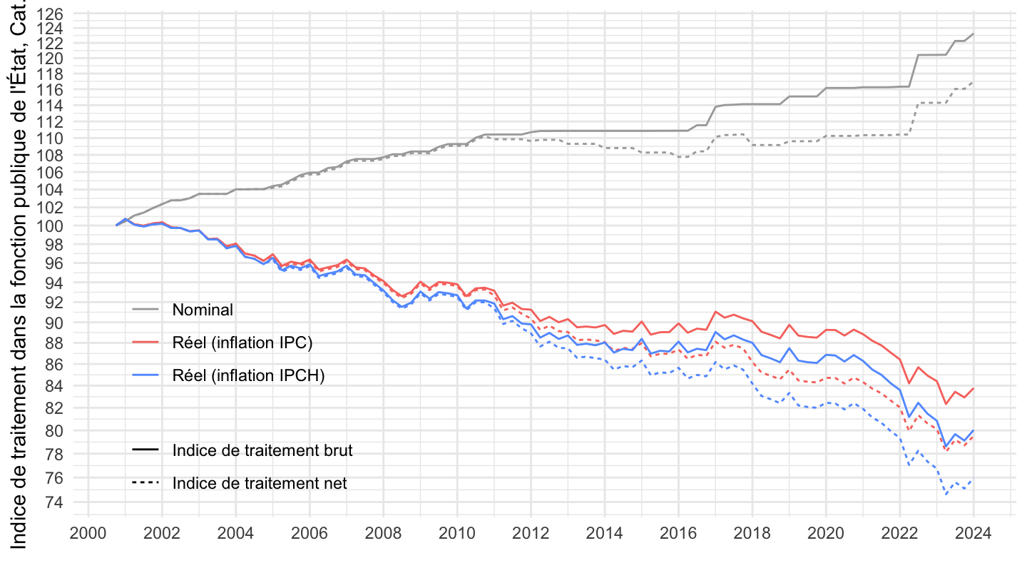
Catégorie B
Nominal
Code
`INDICE-TRAITEMENT-FP` %>%
  filter(CATEGORIE_FP == "B") %>%

  quarter_to_date %>%
  ggplot() + geom_line(aes(x = date, y = OBS_VALUE,  color = Indicateur)) +
  theme_minimal() + ylab("Indice, Catégorie B") + xlab("") +
  scale_x_date(breaks = seq(1920, 2100, 2) %>% paste0("-01-01") %>% as.Date,
               labels = date_format("%Y")) +
  theme(legend.position = c(0.7, 0.2),
        legend.title = element_blank()) +

  scale_y_log10(breaks = seq(0, 200, 1))
Indice Net
Code
`INDICE-TRAITEMENT-FP` %>%
  filter(CATEGORIE_FP == "B",
         INDICATEUR == "NSALNF") %>%

  quarter_to_date %>%
  left_join(inflation, by = "date") %>%
  arrange(date) %>%
  transmute(date, `Indice de traitement net, nominal` = OBS_VALUE,
            `Indice de traitement net, réel` = IPCH[1]*OBS_VALUE/IPCH) %>%
  gather(variable, value, -date) %>%
  ggplot() + geom_line(aes(x = date, y = value,  color = variable)) +
  theme_minimal() + ylab("Indice, Catégorie B") + xlab("") +
  scale_x_date(breaks = seq(1920, 2100, 2) %>% paste0("-01-01") %>% as.Date,
               labels = date_format("%Y")) +
  theme(legend.position = c(0.2, 0.2),
        legend.title = element_blank()) +
  scale_y_log10(breaks = seq(0, 200, 5))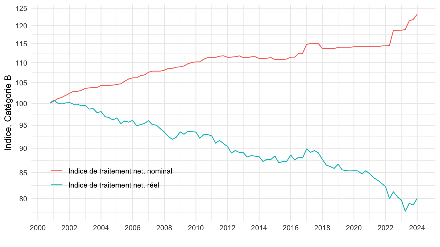
Indice Brut
Code
`INDICE-TRAITEMENT-FP` %>%
  filter(CATEGORIE_FP == "B",
         INDICATEUR == "NSALBF") %>%

  quarter_to_date %>%
  left_join(inflation, by = "date") %>%
  arrange(date) %>%
  transmute(date, `Indice de traitement brut, nominal` = OBS_VALUE,
            `Indice de traitement brut, réel` = IPCH[1]*OBS_VALUE/IPCH) %>%
  gather(variable, value, -date) %>%
  ggplot() + geom_line(aes(x = date, y = value,  color = variable)) +
  theme_minimal() + ylab("Indice, Catégorie B") + xlab("") +
  scale_x_date(breaks = seq(1920, 2100, 2) %>% paste0("-01-01") %>% as.Date,
               labels = date_format("%Y")) +
  theme(legend.position = c(0.2, 0.2),
        legend.title = element_blank()) +
  scale_y_log10(breaks = seq(0, 200, 5))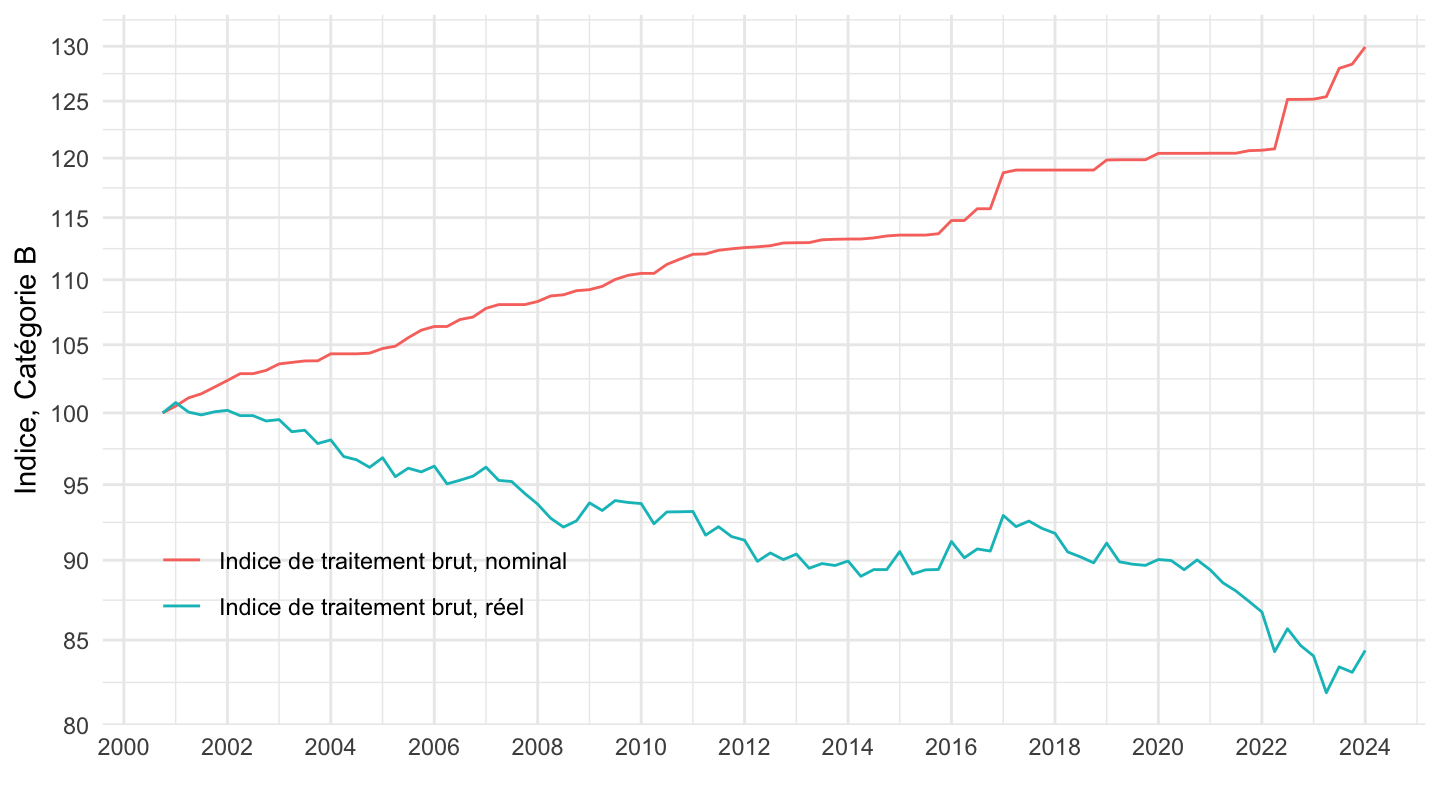
Indice Net/brut
Code
`INDICE-TRAITEMENT-FP` %>%
  filter(CATEGORIE_FP == "B") %>%

  quarter_to_date %>%
  left_join(inflation, by = "date") %>%
  arrange(date) %>%
  transmute(date, Indicateur, `Nominal` = OBS_VALUE,
            `Réel` = IPCH[1]*OBS_VALUE/IPCH) %>%
  gather(variable, value, -date, -Indicateur) %>%
  ggplot() + geom_line(aes(x = date, y = value,  color = variable, linetype = Indicateur)) +
  theme_minimal() + ylab("Indice, Catégorie B") + xlab("") +
  scale_x_date(breaks = seq(1920, 2100, 2) %>% paste0("-01-01") %>% as.Date,
               labels = date_format("%Y")) +
  theme(legend.position = c(0.2, 0.2),
        legend.title = element_blank()) +
  scale_y_log10(breaks = seq(0, 200, 5))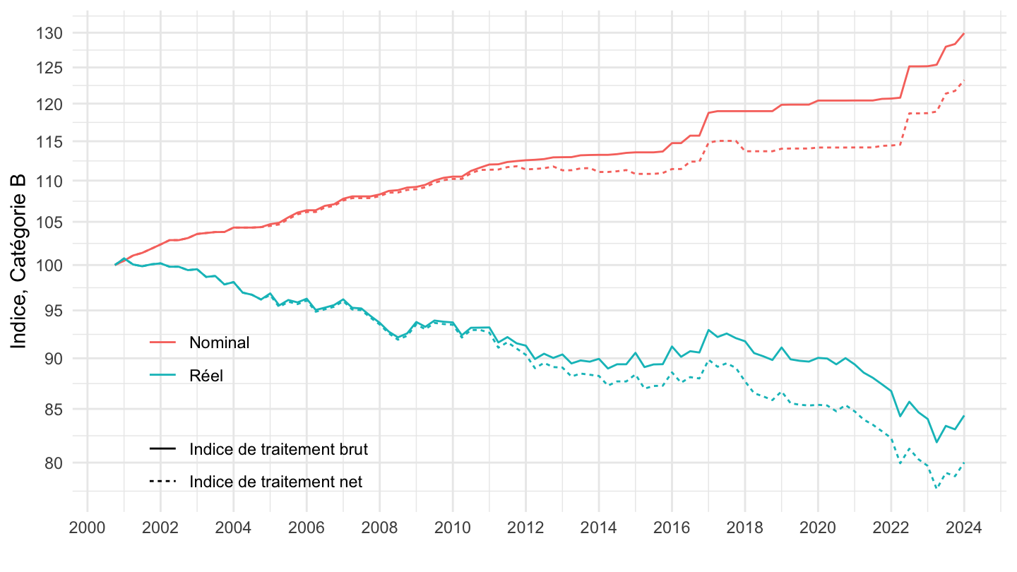
Indice Net/brut, réel IPC IPCH
Code
`INDICE-TRAITEMENT-FP` %>%
  filter(CATEGORIE_FP == "B") %>%

  quarter_to_date %>%
  left_join(inflation, by = "date") %>%
  arrange(date) %>%
  transmute(date, Indicateur,
            `Nominal` = OBS_VALUE,
            `Réel (inflation IPCH)` = IPCH[1]*OBS_VALUE/IPCH,
            `Réel (inflation IPC)` = IPC[1]*OBS_VALUE/IPC) %>%
  gather(variable, value, -date, -Indicateur) %>%
  ggplot() + geom_line(aes(x = date, y = value,  color = variable, linetype = Indicateur)) +
  theme_minimal() + ylab("Indice de traitement dans la fonction publique de l'État, Cat. B") + xlab("") +
  scale_color_manual(values = c("darkgrey", "#F8766D", "#619CFF")) +
  scale_x_date(breaks = seq(1920, 2100, 2) %>% paste0("-01-01") %>% as.Date,
               labels = date_format("%Y")) +
  theme(legend.position = c(0.18, 0.24),
        legend.title = element_blank()) +
  scale_y_log10(breaks = seq(0, 200, 2))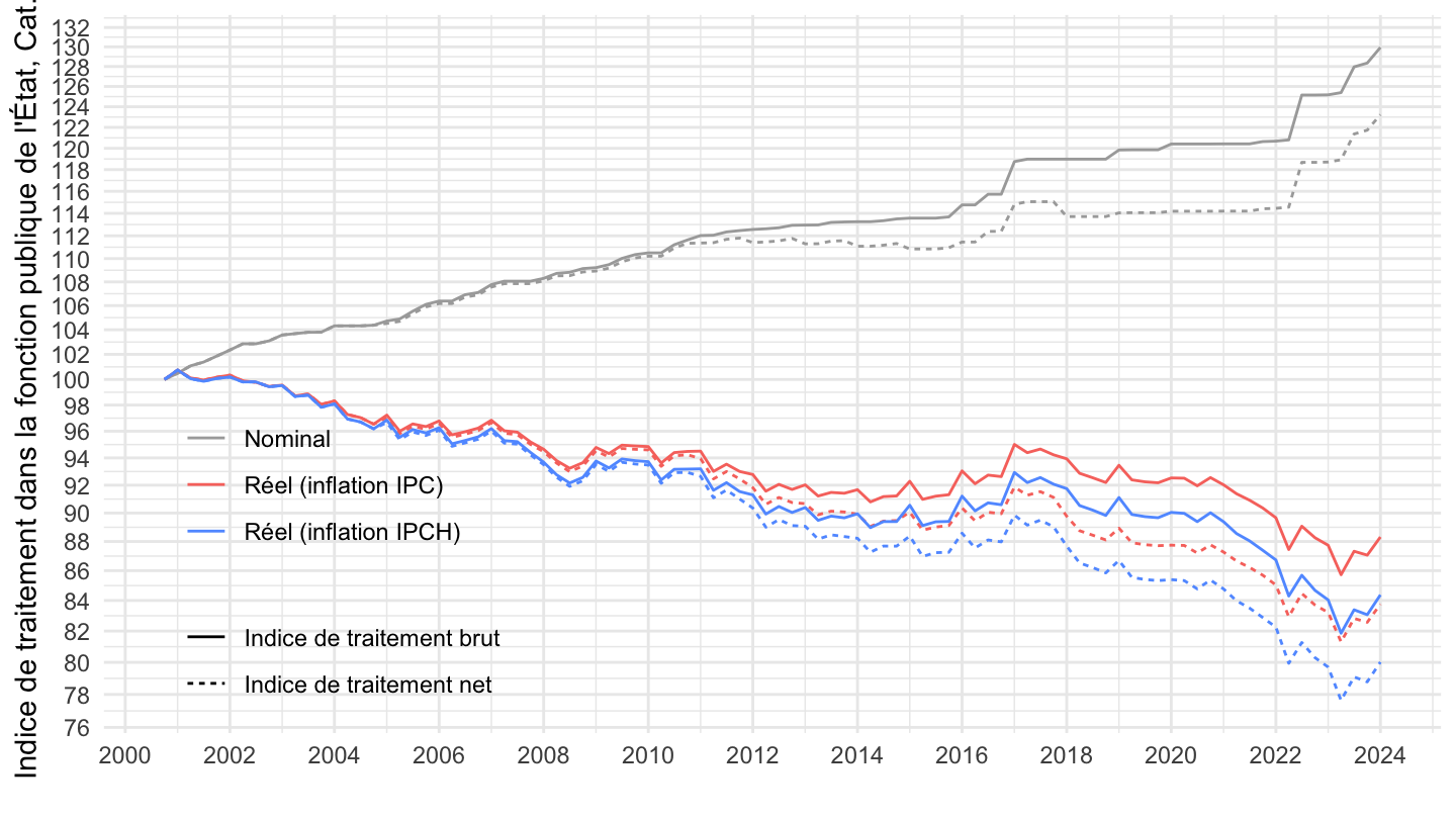
Catégorie C
Nominal
Code
`INDICE-TRAITEMENT-FP` %>%
  filter(CATEGORIE_FP == "B") %>%

  quarter_to_date %>%
  ggplot() + geom_line(aes(x = date, y = OBS_VALUE,  color = Indicateur)) +
  theme_minimal() + ylab("Indice, Catégorie C") + xlab("") +
  scale_x_date(breaks = seq(1920, 2100, 2) %>% paste0("-01-01") %>% as.Date,
               labels = date_format("%Y")) +
  theme(legend.position = c(0.7, 0.2),
        legend.title = element_blank()) +

  scale_y_log10(breaks = seq(0, 200, 1))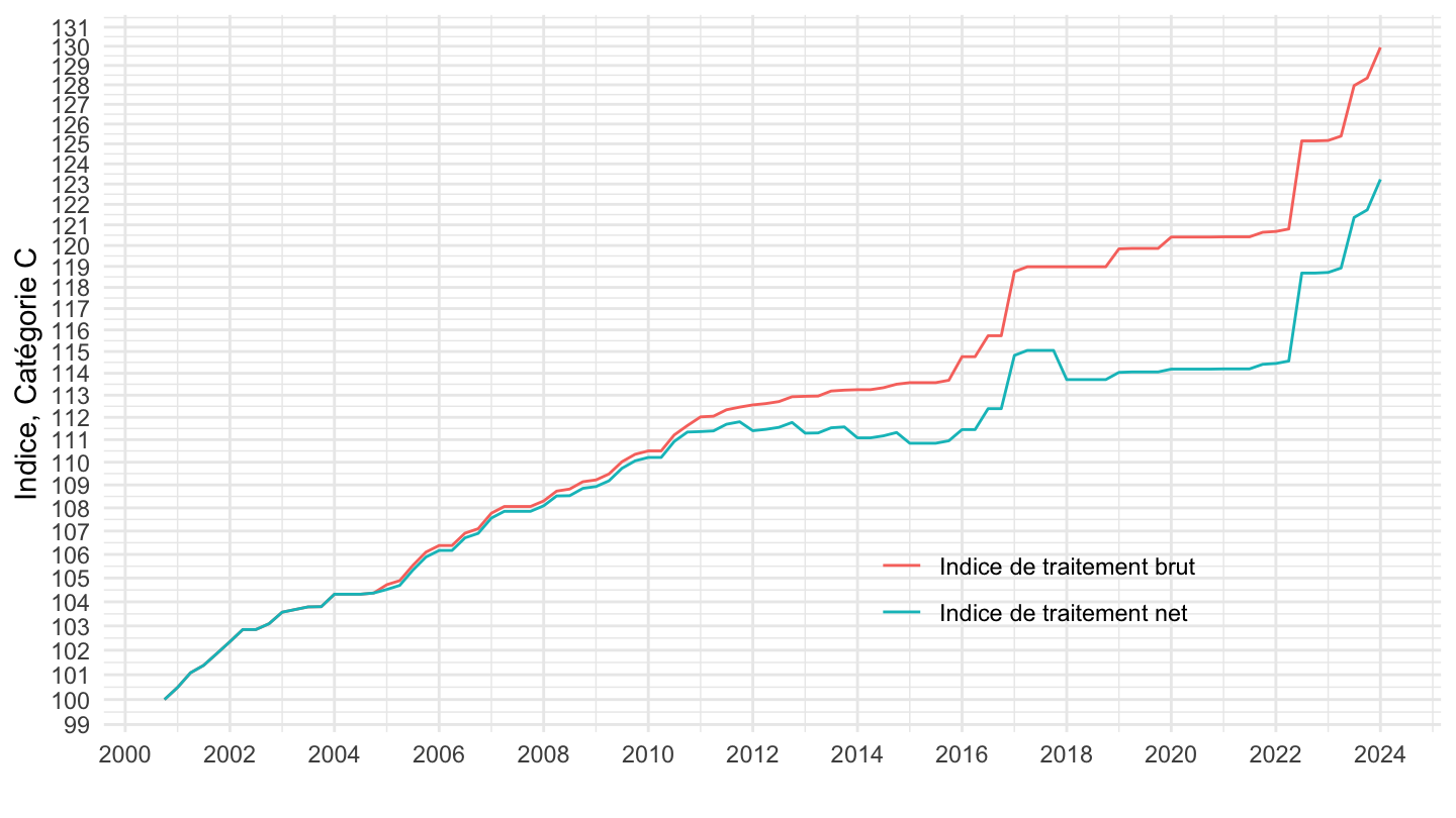
Indice Net
Code
`INDICE-TRAITEMENT-FP` %>%
  filter(CATEGORIE_FP == "C",
         INDICATEUR == "NSALNF") %>%

  quarter_to_date %>%
  left_join(inflation, by = "date") %>%
  arrange(date) %>%
  transmute(date, `Indice de traitement net, nominal` = OBS_VALUE,
            `Indice de traitement net, réel` = IPCH[1]*OBS_VALUE/IPCH) %>%
  gather(variable, value, -date) %>%
  ggplot() + geom_line(aes(x = date, y = value,  color = variable)) +
  theme_minimal() + ylab("Indice, Catégorie C") + xlab("") +
  scale_x_date(breaks = seq(1920, 2100, 2) %>% paste0("-01-01") %>% as.Date,
               labels = date_format("%Y")) +
  theme(legend.position = c(0.2, 0.2),
        legend.title = element_blank()) +
  scale_y_log10(breaks = seq(0, 200, 5))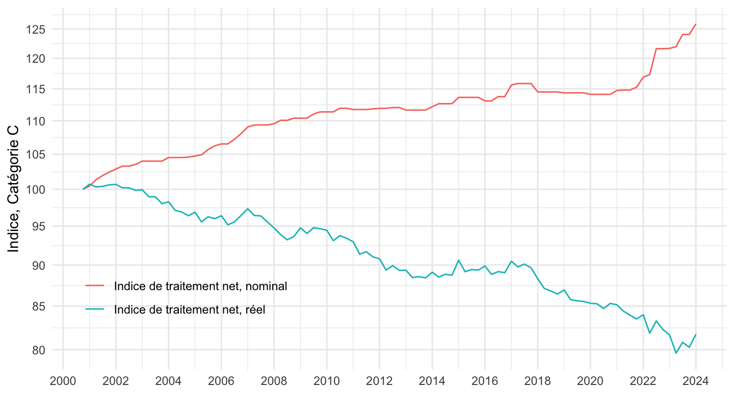
Indice Brut
Code
`INDICE-TRAITEMENT-FP` %>%
  filter(CATEGORIE_FP == "C",
         INDICATEUR == "NSALBF") %>%

  quarter_to_date %>%
  left_join(inflation, by = "date") %>%
  arrange(date) %>%
  transmute(date, `Indice de traitement brut, nominal` = OBS_VALUE,
            `Indice de traitement brut, réel` = IPCH[1]*OBS_VALUE/IPCH) %>%
  gather(variable, value, -date) %>%
  ggplot() + geom_line(aes(x = date, y = value,  color = variable)) +
  theme_minimal() + ylab("Indice, Catégorie C") + xlab("") +
  scale_x_date(breaks = seq(1920, 2100, 2) %>% paste0("-01-01") %>% as.Date,
               labels = date_format("%Y")) +
  theme(legend.position = c(0.2, 0.2),
        legend.title = element_blank()) +
  scale_y_log10(breaks = seq(0, 200, 5))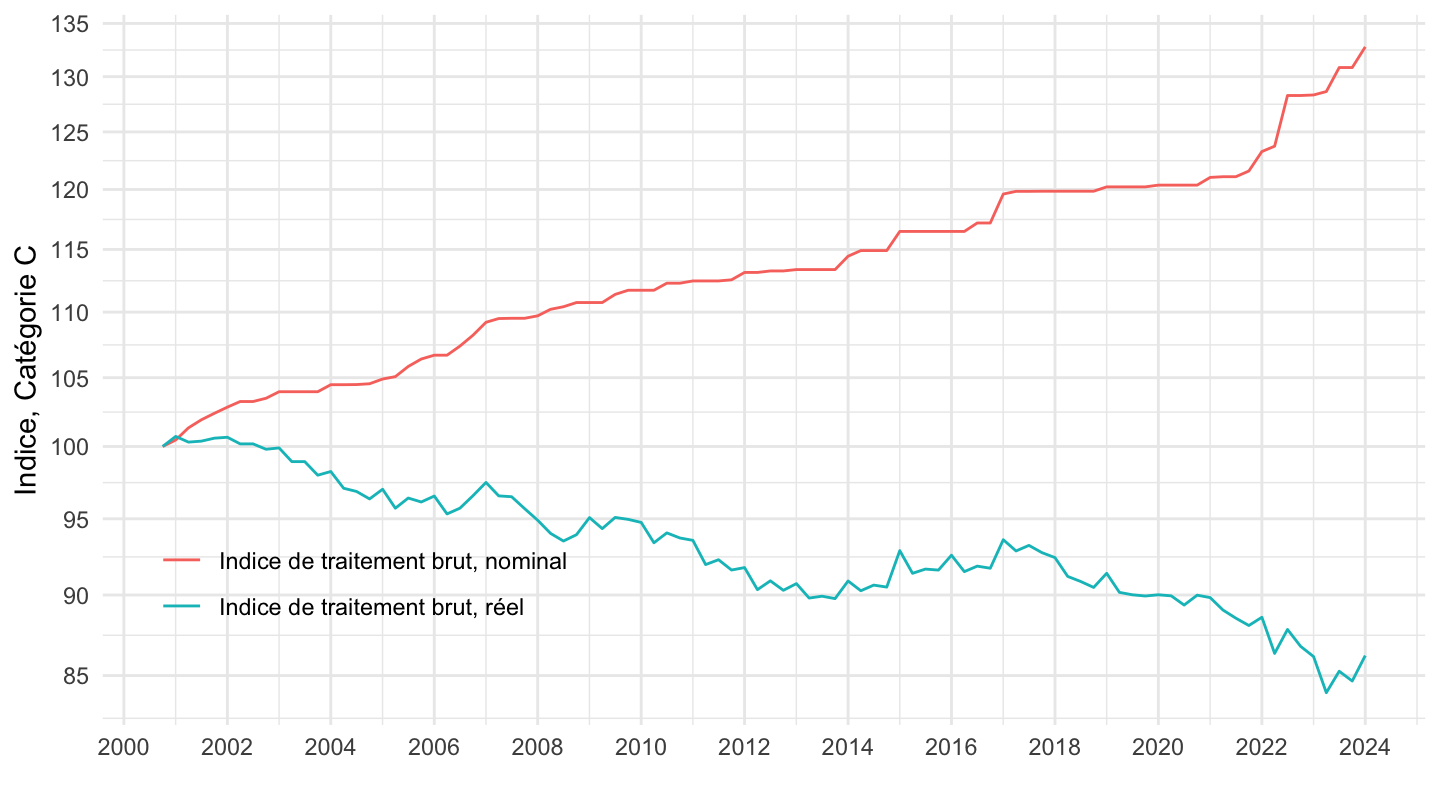
Indice Net/brut, réel IPC IPCH
Code
`INDICE-TRAITEMENT-FP` %>%
  filter(CATEGORIE_FP == "C") %>%

  quarter_to_date %>%
  left_join(inflation, by = "date") %>%
  arrange(date) %>%
  transmute(date, Indicateur,
            `Nominal` = OBS_VALUE,
            `Réel (inflation IPCH)` = IPCH[1]*OBS_VALUE/IPCH,
            `Réel (inflation IPC)` = IPC[1]*OBS_VALUE/IPC) %>%
  gather(variable, value, -date, -Indicateur) %>%
  ggplot() + geom_line(aes(x = date, y = value,  color = variable, linetype = Indicateur)) +
  theme_minimal() + ylab("Indice de traitement dans la fonction publique de l'État, Cat. C") + xlab("") +
  scale_color_manual(values = c("darkgrey", "#F8766D", "#619CFF")) +
  scale_x_date(breaks = seq(1920, 2100, 2) %>% paste0("-01-01") %>% as.Date,
               labels = date_format("%Y")) +
  theme(legend.position = c(0.18, 0.24),
        legend.title = element_blank()) +
  scale_y_log10(breaks = seq(0, 200, 2))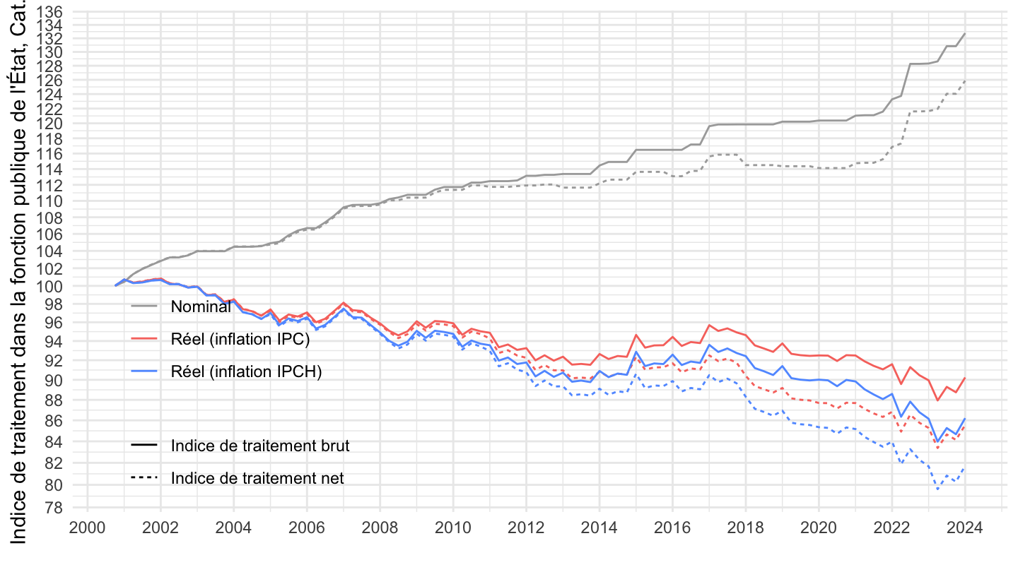
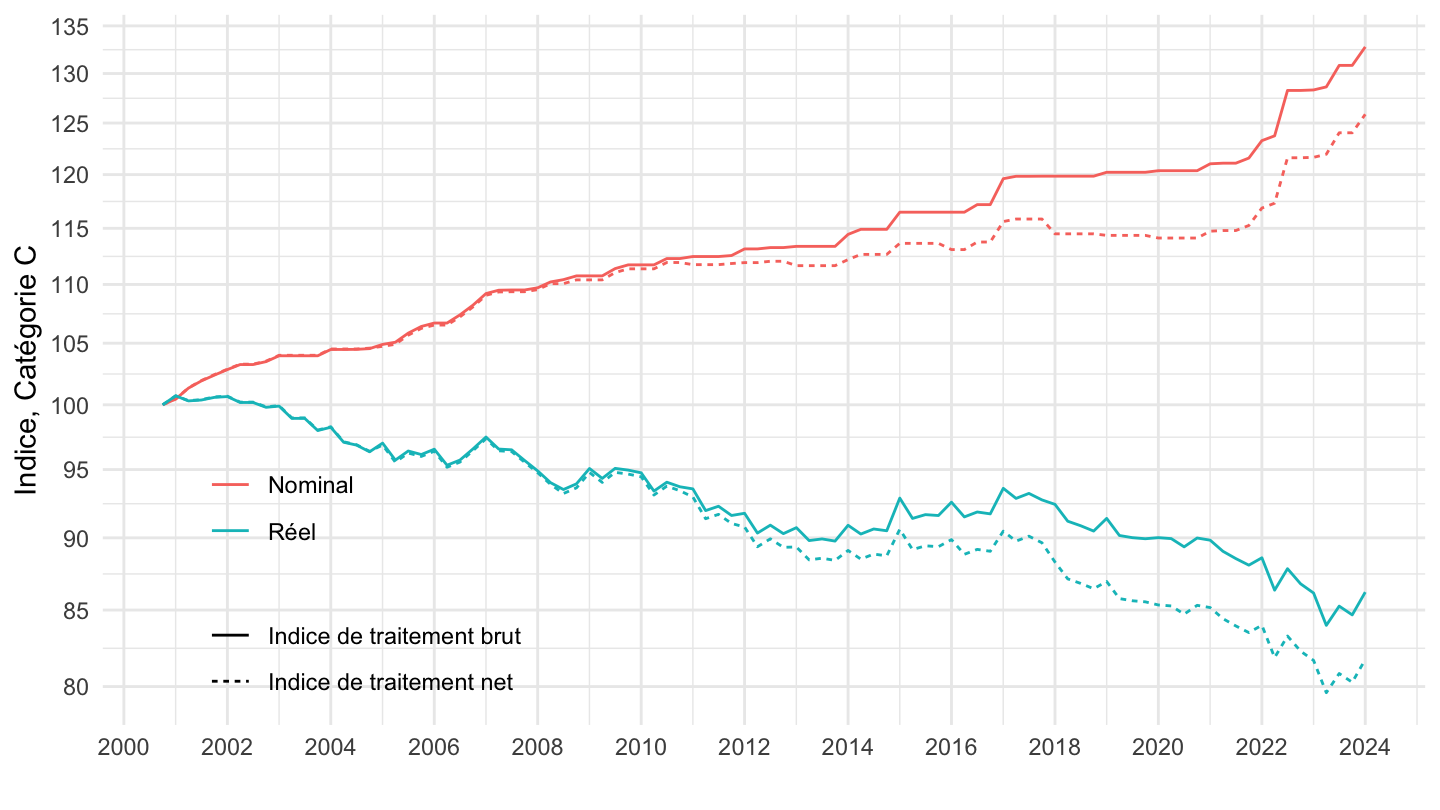
Indice Net/brut
Code
`INDICE-TRAITEMENT-FP` %>%
  filter(CATEGORIE_FP == "C") %>%

  quarter_to_date %>%
  left_join(inflation, by = "date") %>%
  arrange(date) %>%
  transmute(date, Indicateur, `Nominal` = OBS_VALUE,
            `Réel` = IPCH[1]*OBS_VALUE/IPCH) %>%
  gather(variable, value, -date, -Indicateur) %>%
  ggplot() + geom_line(aes(x = date, y = value,  color = variable, linetype = Indicateur)) +
  theme_minimal() + ylab("Indice, Catégorie C") + xlab("") +
  scale_x_date(breaks = seq(1920, 2100, 2) %>% paste0("-01-01") %>% as.Date,
               labels = date_format("%Y")) +
  theme(legend.position = c(0.2, 0.2),
        legend.title = element_blank()) +
  scale_y_log10(breaks = seq(0, 200, 5))