Analytical house prices indicators
Data - OECD
Info
Last observation: Quarterly: 2026-Q1 (N = 30) · Annual: 2025 (N = 132)
Last update of .RData: 12 avr 2026, 12:21. Last compile: 25 jul 2026, 00:24
Structure
Rent Prices - RPI
United States, Japan, Canada
Code
HOUSE_PRICES %>%
  filter(MEASURE == "RPI",
         REF_AREA %in% c("USA", "JPN", "CAN"),
         substr(obsTime, 6, 6) != "Q") %>%
  left_join(colors, by = c("Ref_area" = "country")) %>%
  year_to_date() %>%
  ggplot(.) + theme_minimal() + xlab("") + ylab("Rent Prices") +
  geom_line(aes(x = date, y = obsValue, color = color)) +
  scale_x_date(breaks = seq(1900, 2100, 5) %>% paste0("-01-01") %>% as.Date,
               labels = date_format("%Y")) +
  scale_y_log10(breaks = seq(0, 600, 10),
                     labels = dollar_format(a = 1, prefix = "")) +
  scale_color_identity() + add_3flags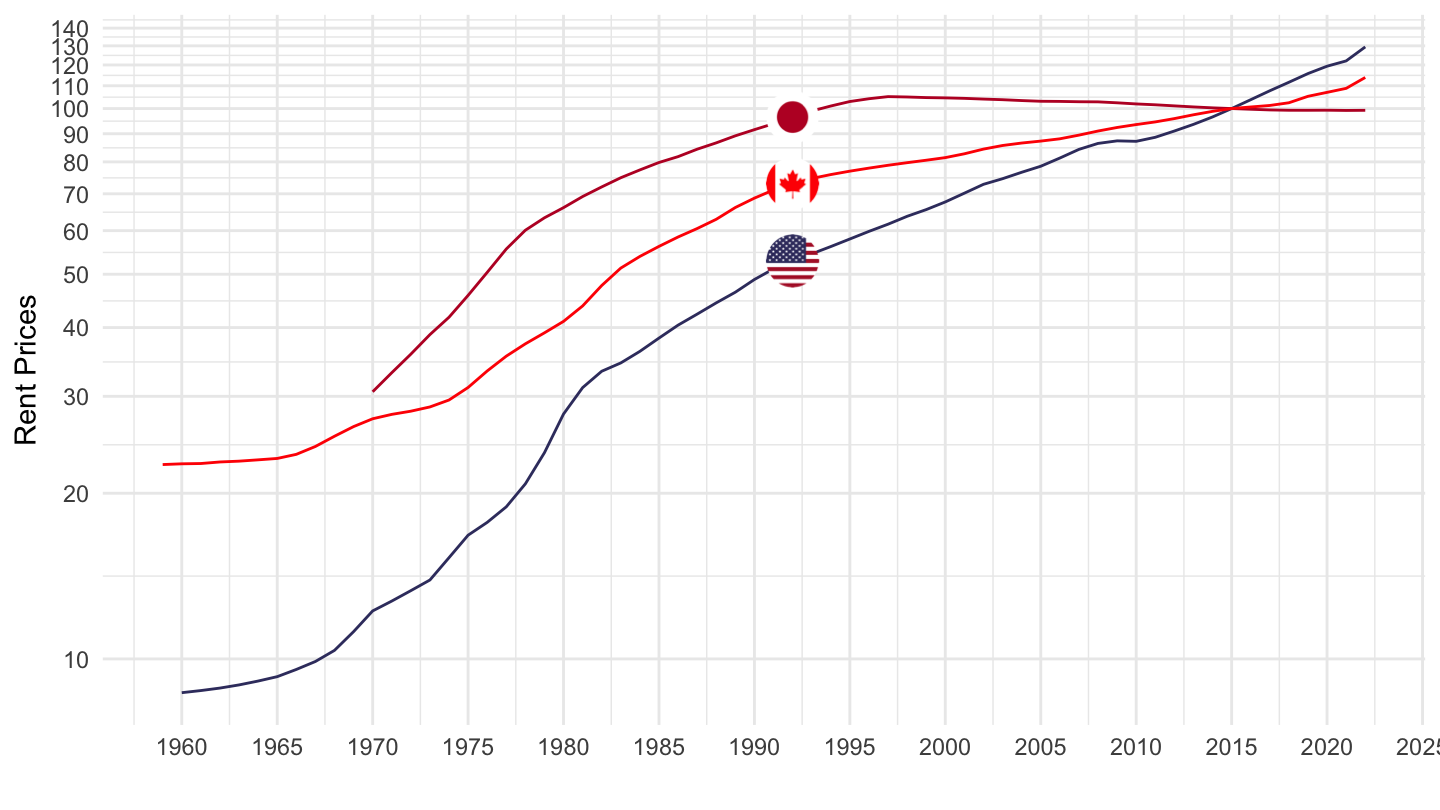
France, Spain, Italy
Code
HOUSE_PRICES %>%
  filter(MEASURE == "RPI",
         REF_AREA %in% c("FRA", "ITA", "ESP"),
         substr(obsTime, 6, 6) != "Q") %>%
  left_join(colors, by = c("Ref_area" = "country")) %>%
  year_to_date() %>%
  ggplot(.) + theme_minimal() + xlab("") + ylab("Rent Prices") +
  geom_line(aes(x = date, y = obsValue, color = color)) +
  scale_x_date(breaks = seq(1900, 2100, 5) %>% paste0("-01-01") %>% as.Date,
               labels = date_format("%Y")) +
  scale_y_log10(breaks = seq(0, 600, 10),
                     labels = dollar_format(a = 1, prefix = "")) +
  scale_color_identity() + add_3flags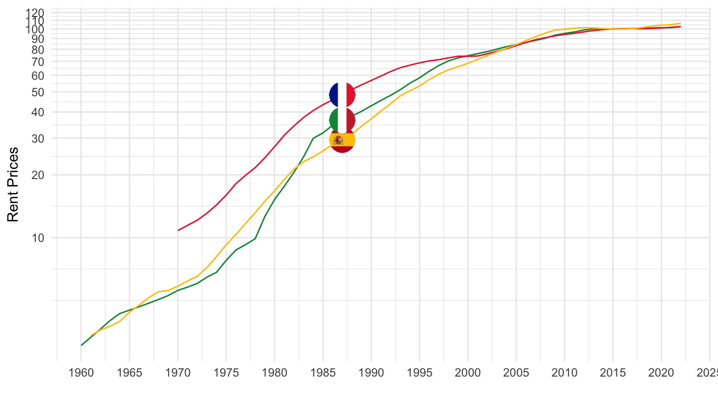
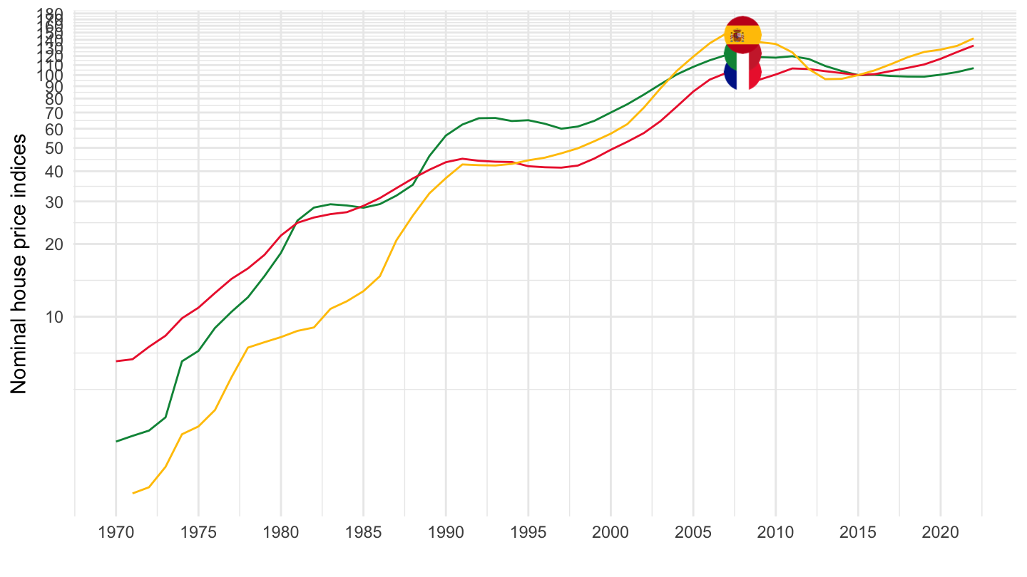
Nominal house price indices, s.a. - HPI
United States, Japan, Canada
Code
HOUSE_PRICES %>%
  filter(MEASURE == "HPI",
         REF_AREA %in% c("USA", "JPN", "CAN"),
         substr(obsTime, 6, 6) != "Q") %>%
  left_join(colors, by = c("Ref_area" = "country")) %>%
  year_to_date() %>%
  ggplot(.) + theme_minimal() + xlab("") + ylab("Nominal House Prices") +
  geom_line(aes(x = date, y = obsValue, color = color)) +
  scale_x_date(breaks = seq(1900, 2100, 5) %>% paste0("-01-01") %>% as.Date,
               labels = date_format("%Y")) +
  scale_y_log10(breaks = seq(0, 600, 10),
                     labels = dollar_format(a = 1, prefix = "")) +
  scale_color_identity() + add_3flags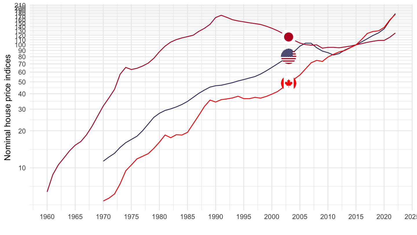
France, Spain, Italy
Code
HOUSE_PRICES %>%
  filter(MEASURE == "HPI",
         REF_AREA %in% c("FRA", "ESP", "ITA"),
         substr(obsTime, 6, 6) != "Q") %>%
  left_join(colors, by = c("Ref_area" = "country")) %>%
  year_to_date() %>%
  ggplot(.) + theme_minimal() + xlab("") + ylab("Nominal House Prices") +
  geom_line(aes(x = date, y = obsValue, color = color)) +
  scale_x_date(breaks = seq(1900, 2100, 5) %>% paste0("-01-01") %>% as.Date,
               labels = date_format("%Y")) +
  scale_y_log10(breaks = seq(0, 600, 10),
                     labels = dollar_format(a = 1, prefix = "")) +
  scale_color_identity() + add_3flags