
Last compile: 24 oct. 2026, 01:06
Indice Fonction Publique
All
Valeur
Code
indicefp |>
  select(date, point_indice_en_euros) |>
  gather(variable, value, -date) |>
  group_by(variable) |>
  complete(date = seq.Date(min(date), max(date), by = "day")) |>
  fill(value) |>
  ggplot() + geom_line(aes(x = date, y = value)) +
  scale_color_manual(values = viridis(8)[1:7]) +
  theme_minimal() +
  scale_x_date(breaks = seq(1920, 2100, 5) |> paste0("-01-01") |> as.Date(),
               labels = date_format("%Y")) +
  theme(legend.position = c(0.3, 0.8),
        legend.title = element_blank()) +
  scale_y_log10(breaks = seq(0, 200, 5),
                     labels = dollar_format(accuracy = 1, suffix = " € / point", prefix = "")) +
  ylab("Point Indice Fonction Publique (euros)") + xlab("")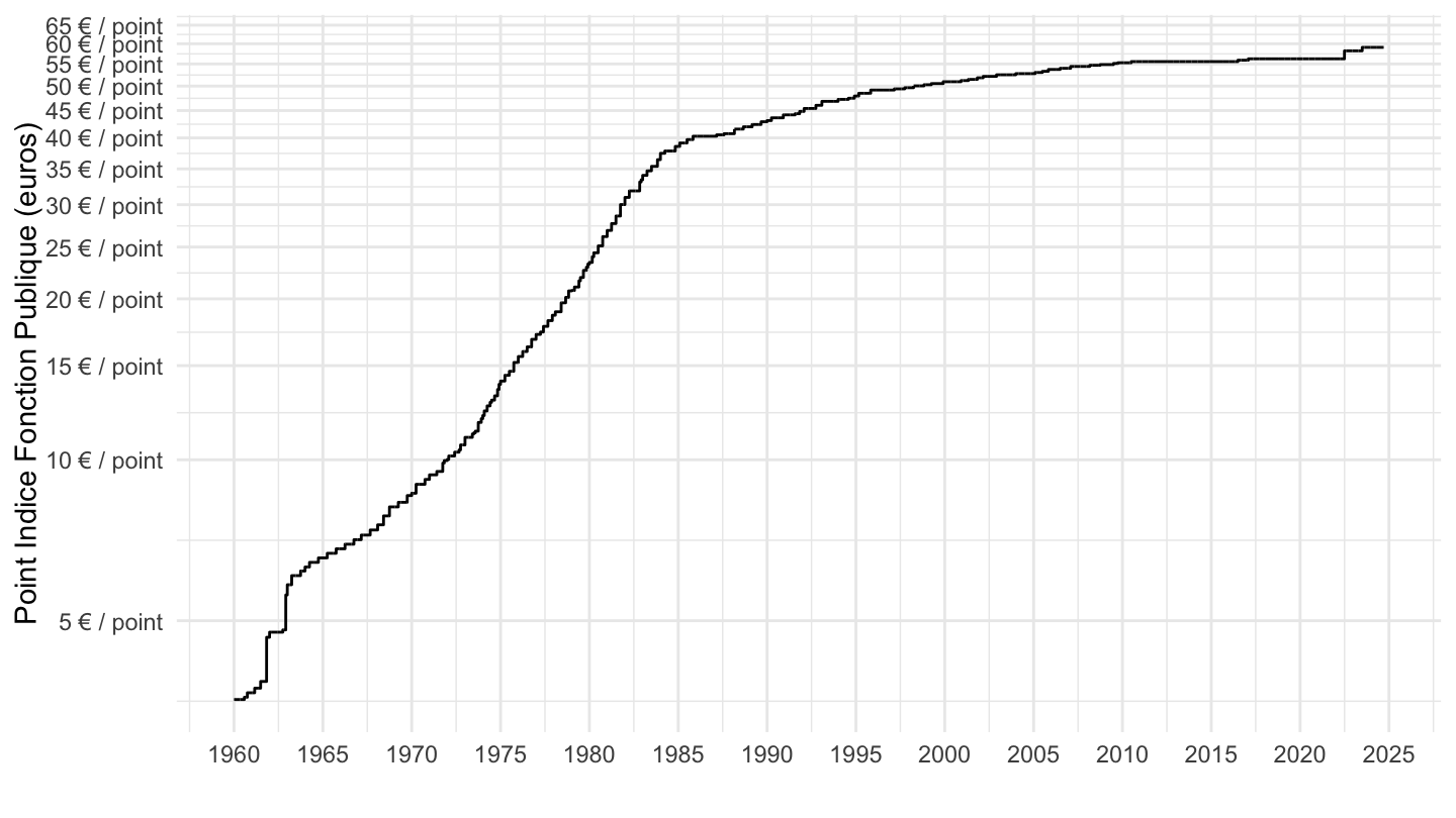
Base 100
Code
indicefp |>
  select(date, point_indice_en_euros) |>
  gather(variable, value, -date) |>
  group_by(variable) |>
  complete(date = seq.Date(min(date), max(date), by = "day")) |>
  fill(value) |>
  mutate(value = 100*value/value[1]) |>
  ggplot() + geom_line(aes(x = date, y = value)) +
  theme_minimal() +
  scale_x_date(breaks = seq(1920, 2100, 5) |> paste0("-01-01") |> as.Date(),
               labels = date_format("%Y")) +
  theme(legend.position = c(0.3, 0.8),
        legend.title = element_blank()) +
  scale_y_log10(breaks = seq(0, 3000, 100)) +
  ylab("Point Indice Fonction Publique") + xlab("")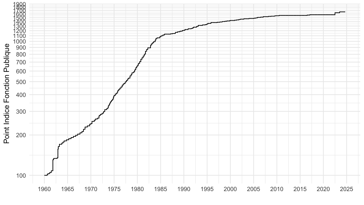
1970-1990
Valeur
Code
indicefp |>
  select(date, point_indice_en_euros) |>
  gather(variable, value, -date) |>
  group_by(variable) |>
  complete(date = seq.Date(min(date), max(date), by = "day")) |>
  fill(value) |>
  filter(date >= as.Date("1970-01-01"),
         date <= as.Date("1990-01-01")) |>
  ggplot() + geom_line(aes(x = date, y = value)) +
  theme_minimal() + ylab("Point Indice Fonction Publique (euros)") + xlab("") +
  scale_x_date(breaks = seq(1920, 2100, 2) |> paste0("-01-01") |> as.Date(),
               labels = date_format("%Y")) +
  scale_y_log10(breaks = seq(0, 200, 4),
                     labels = dollar_format(accuracy = 1, suffix = " € / point", prefix = ""))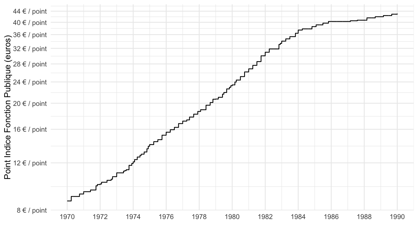
Base 100
Code
indicefp |>
  select(date, point_indice_en_euros) |>
  gather(variable, value, -date) |>
  group_by(variable) |>
  complete(date = seq.Date(min(date), max(date), by = "day")) |>
  fill(value) |>
  filter(date >= as.Date("1970-01-01"),
         date <= as.Date("1990-01-01")) |>
  mutate(value = 100*value/value[1]) |>
  ggplot() + geom_line(aes(x = date, y = value)) +
  theme_minimal() + ylab("Point Indice Fonction Publique") + xlab("") +
  scale_x_date(breaks = seq(1920, 2100, 2) |> paste0("-01-01") |> as.Date(),
               labels = date_format("%Y")) +
  scale_y_log10(breaks = seq(0, 1000, 20))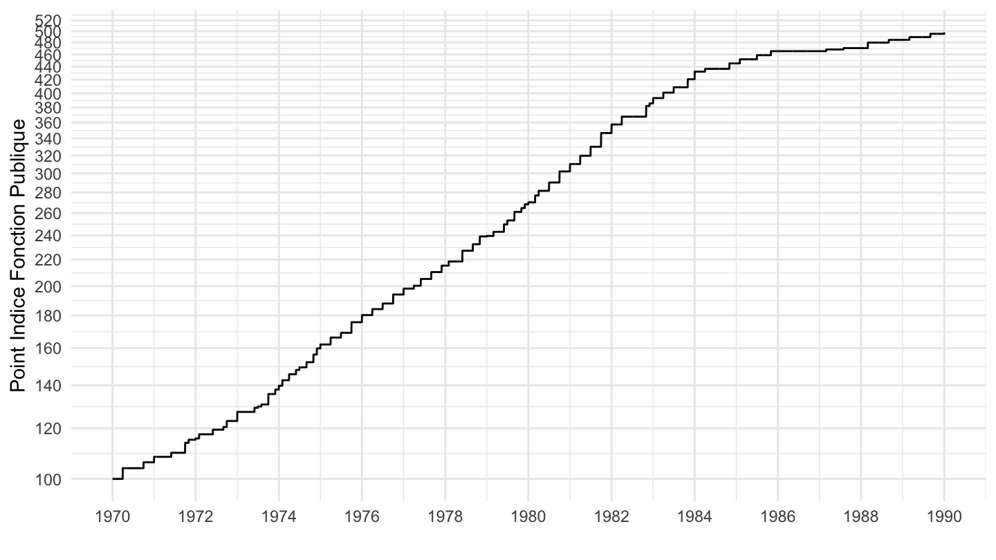
1986-
Valeur
Code
indicefp |>
  arrange(desc(date)) |>
  # Add today's date to be equal ------
  slice(1, 1:n()) |>
  mutate(date = ifelse(row_number() == 1, Sys.Date(), date)) |>
  mutate(date = as.Date(date)) |>
  select(date, point_indice_en_euros) |>
  gather(variable, value, -date) |>
  group_by(variable) |>
  complete(date = seq.Date(min(date), max(date), by = "day")) |>
  fill(value) |>
  filter(date >= as.Date("1986-01-01")) |>
  ggplot() + geom_line(aes(x = date, y = value)) +
  theme_minimal() + ylab("Point Indice Fonction Publique (euros)") + xlab("") +
  scale_x_date(breaks = seq(1920, 2100, 5) |> paste0("-01-01") |> as.Date(),
               labels = date_format("%Y")) +
  scale_y_log10(breaks = seq(0, 200, 1),
                     labels = dollar_format(accuracy = 1, suffix = " € / point", prefix = ""))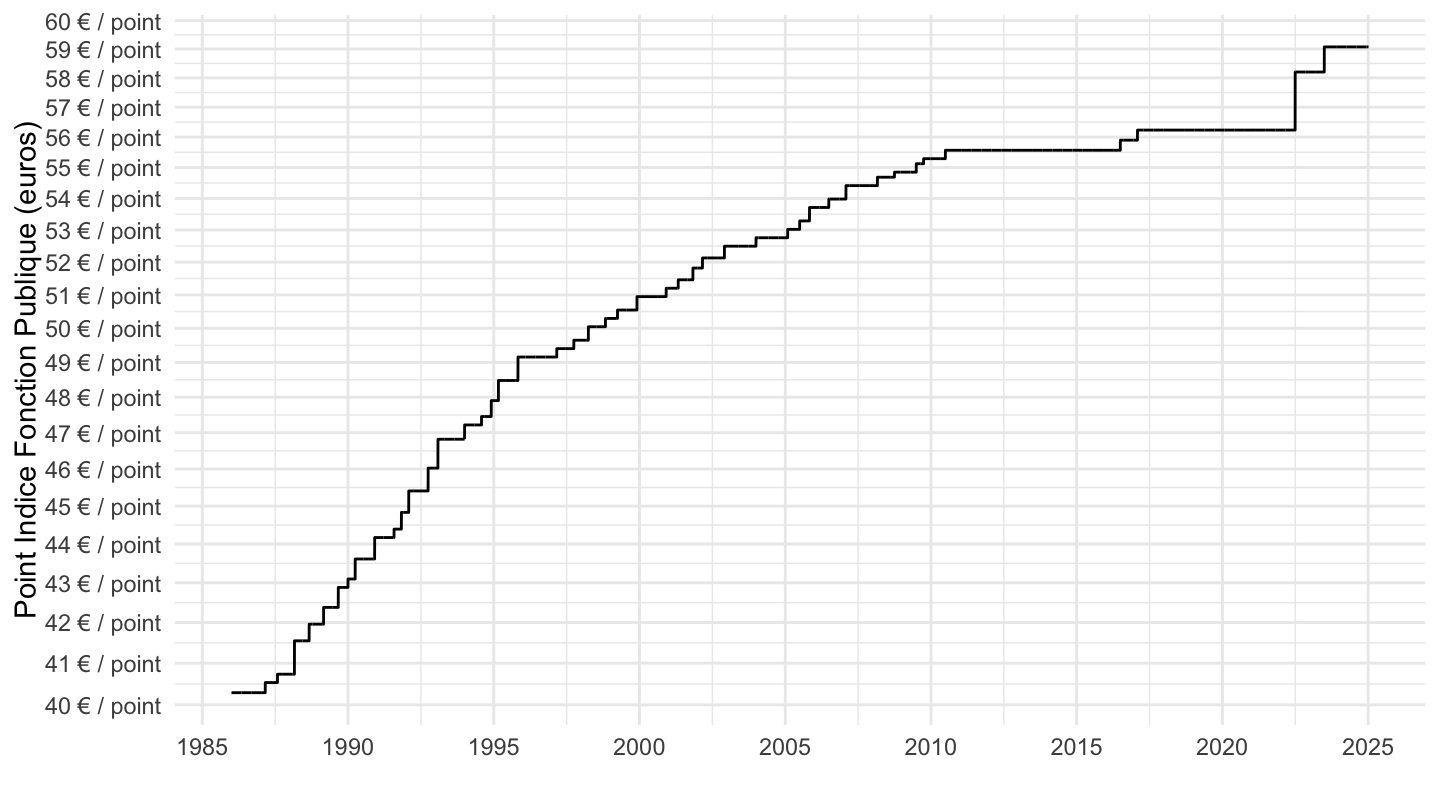
Base 100
Code
indicefp |>
  select(date, point_indice_en_euros) |>
  gather(variable, value, -date) |>
  group_by(variable) |>
  complete(date = seq.Date(min(date), max(date), by = "day")) |>
  fill(value) |>
  filter(date >= as.Date("1986-01-01")) |>
  mutate(value = 100*value/value[1]) |>
  ggplot() + geom_line(aes(x = date, y = value)) +
  theme_minimal() + ylab("Point Indice Fonction Publique") + xlab("") +
  scale_x_date(breaks = seq(1920, 2100, 5) |> paste0("-01-01") |> as.Date(),
               labels = date_format("%Y")) +
  scale_y_log10(breaks = seq(0, 200, 5))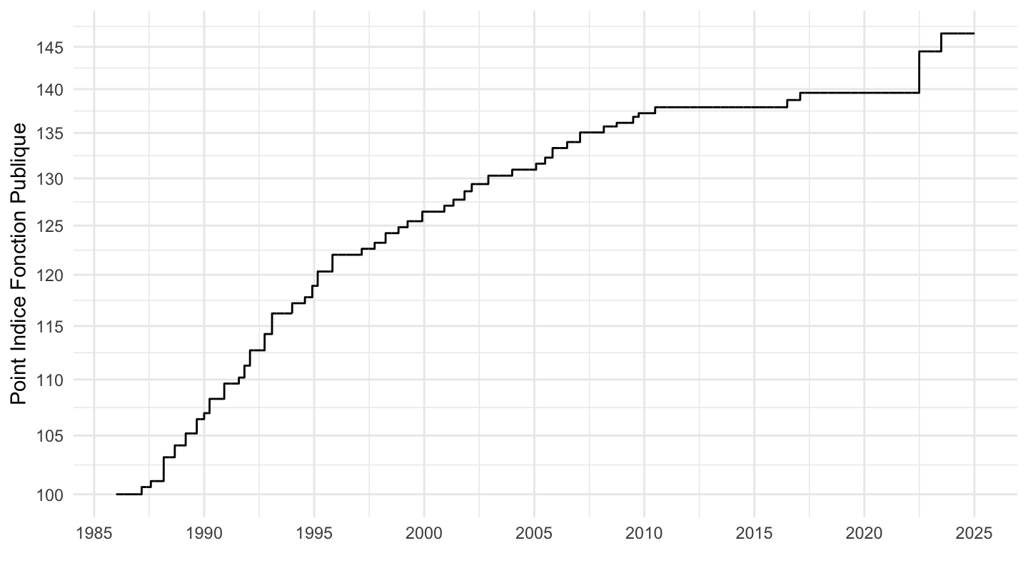
1990-
Valeur
Code
indicefp |>
  select(date, point_indice_en_euros) |>
  gather(variable, value, -date) |>
  group_by(variable) |>
  complete(date = seq.Date(min(date), max(date), by = "day")) |>
  fill(value) |>
  filter(date >= as.Date("1990-01-01")) |>
  ggplot() + geom_line(aes(x = date, y = value)) +
  theme_minimal() + ylab("Point Indice Fonction Publique (euros)") + xlab("") +
  scale_x_date(breaks = seq(1920, 2100, 2) |> paste0("-01-01") |> as.Date(),
               labels = date_format("%Y")) +
  scale_y_log10(breaks = seq(0, 200, 1),
                     labels = dollar_format(accuracy = 1, suffix = " € / point", prefix = ""))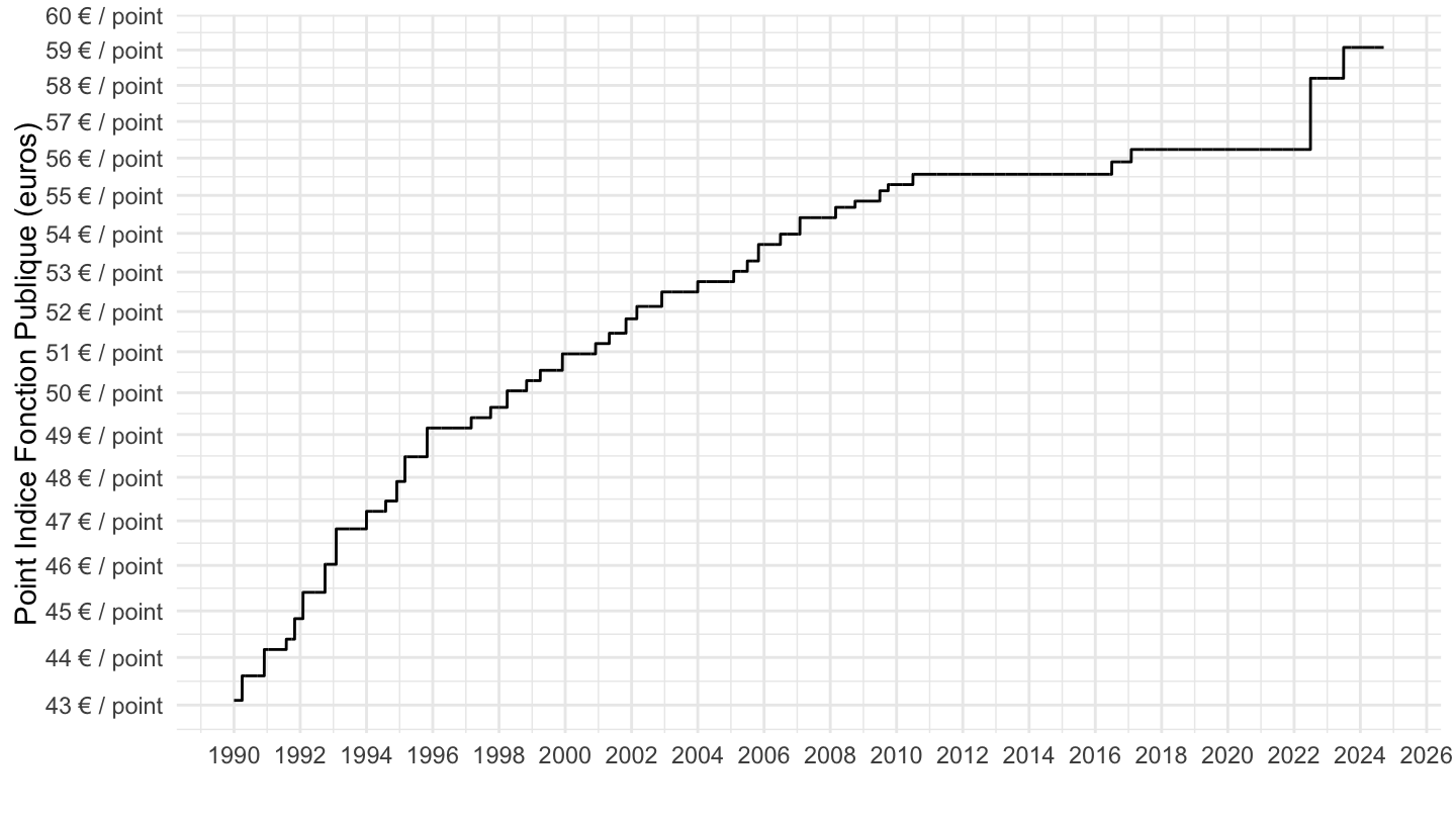
Base 100
Code
indicefp |>
  select(date, point_indice_en_euros) |>
  gather(variable, value, -date) |>
  group_by(variable) |>
  complete(date = seq.Date(min(date), max(date), by = "day")) |>
  fill(value) |>
  filter(date >= as.Date("1990-01-01")) |>
  mutate(value = 100*value/value[1]) |>
  ggplot() + geom_line(aes(x = date, y = value)) +
  theme_minimal() + ylab("Point Indice Fonction Publique") + xlab("") +
  scale_x_date(breaks = seq(1920, 2100, 2) |> paste0("-01-01") |> as.Date(),
               labels = date_format("%Y")) +
  scale_y_log10(breaks = seq(0, 200, 5))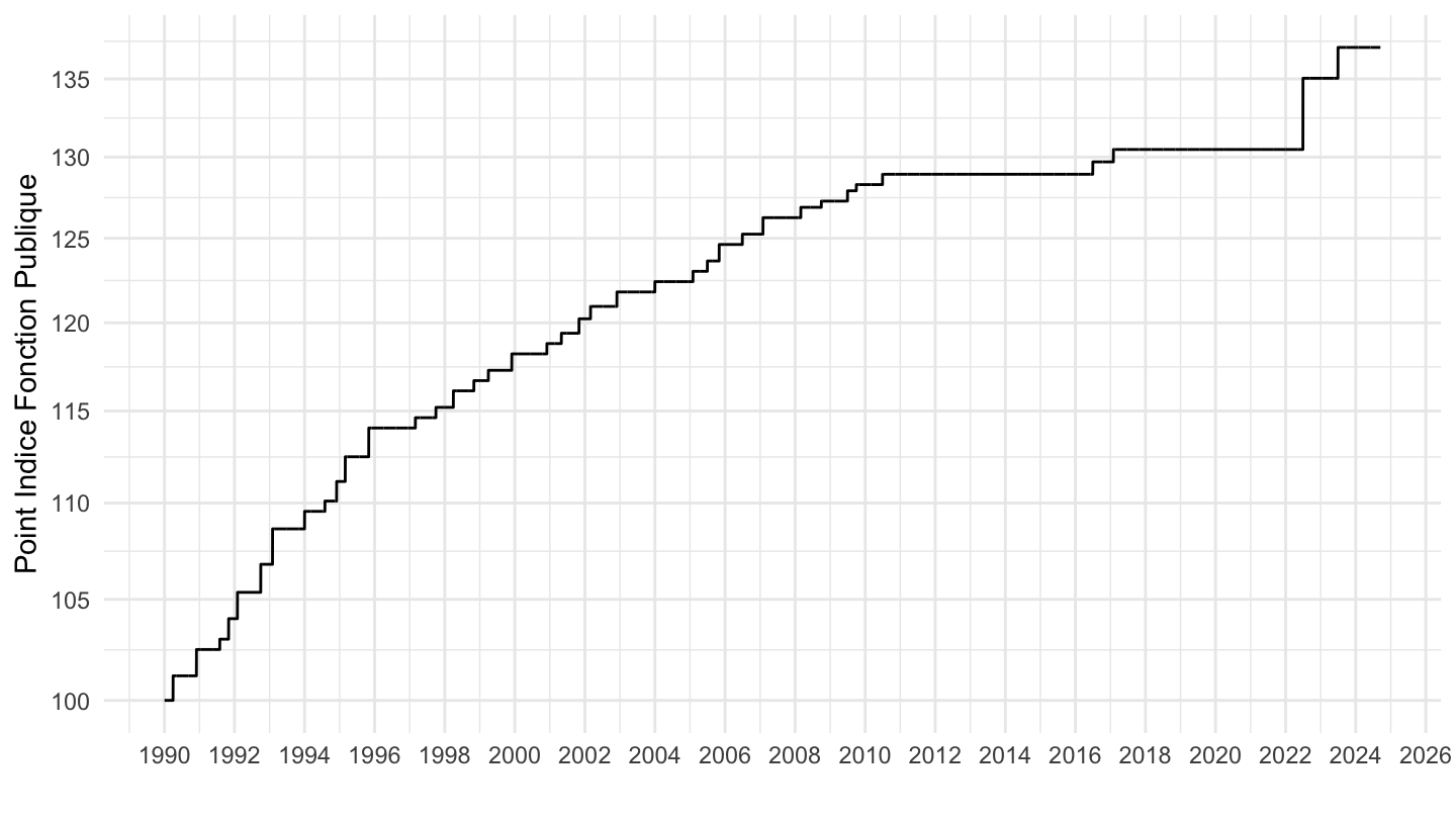
1992-
Valeur
Code
indicefp |>
  select(date, point_indice_en_euros) |>
  gather(variable, value, -date) |>
  group_by(variable) |>
  complete(date = seq.Date(min(date), max(date), by = "day")) |>
  fill(value) |>
  filter(date >= as.Date("1992-01-01")) |>
  ggplot() + geom_line(aes(x = date, y = value)) +
  theme_minimal() + ylab("Point Indice Fonction Publique (euros)") + xlab("") +
  scale_x_date(breaks = seq(1920, 2100, 2) |> paste0("-01-01") |> as.Date(),
               labels = date_format("%Y")) +
  scale_y_log10(breaks = seq(0, 200, 1),
                     labels = dollar_format(accuracy = 1, suffix = " € / point", prefix = ""))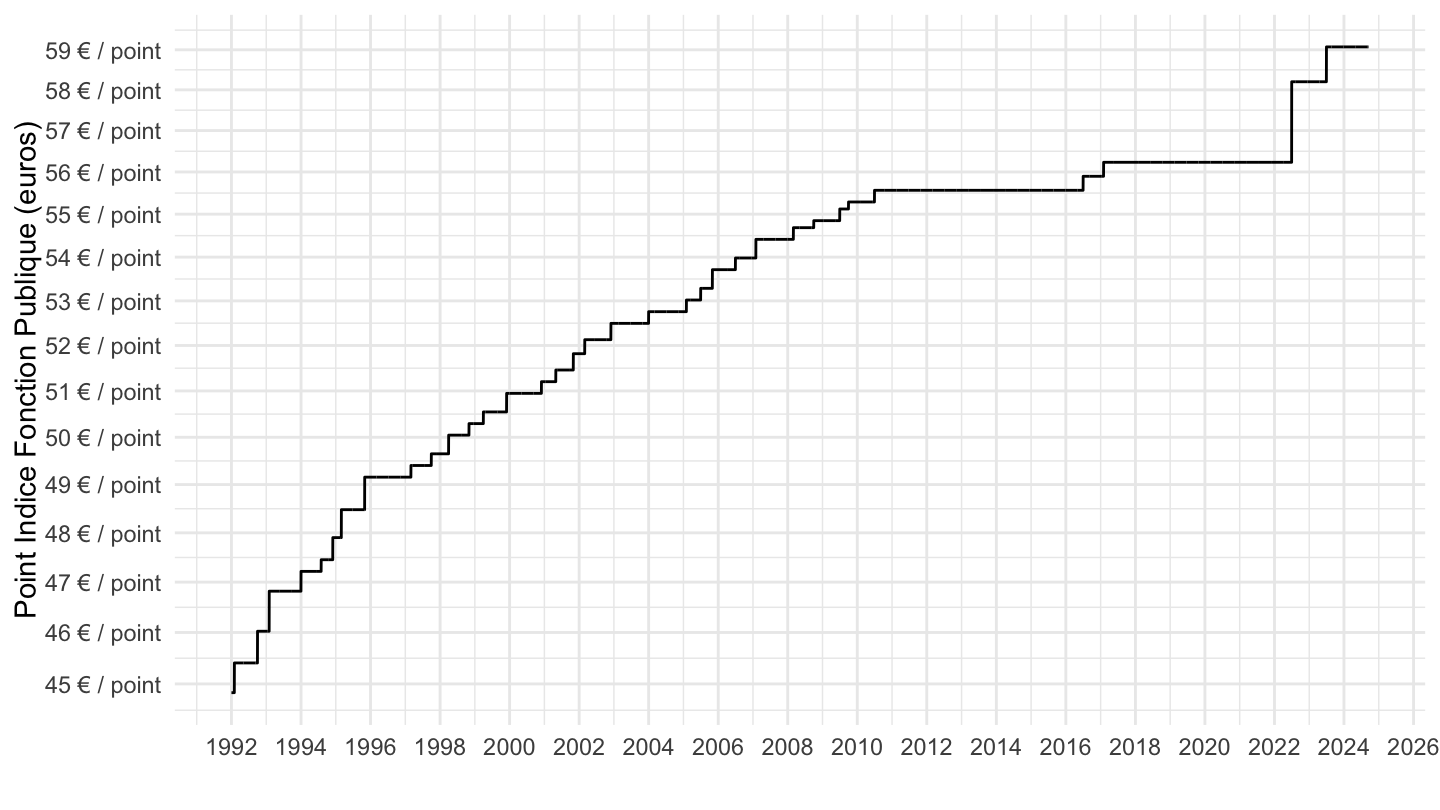
Base 100
Code
indicefp |>
  select(date, point_indice_en_euros) |>
  gather(variable, value, -date) |>
  group_by(variable) |>
  complete(date = seq.Date(min(date), max(date), by = "day")) |>
  fill(value) |>
  filter(date >= as.Date("1992-01-01")) |>
  mutate(value = 100*value/value[1]) |>
  ggplot() + geom_line(aes(x = date, y = value)) +
  theme_minimal() + ylab("Point Indice Fonction Publique (euros)") + xlab("") +
  scale_x_date(breaks = seq(1920, 2100, 2) |> paste0("-01-01") |> as.Date(),
               labels = date_format("%Y")) +
  scale_y_log10(breaks = seq(0, 200, 5))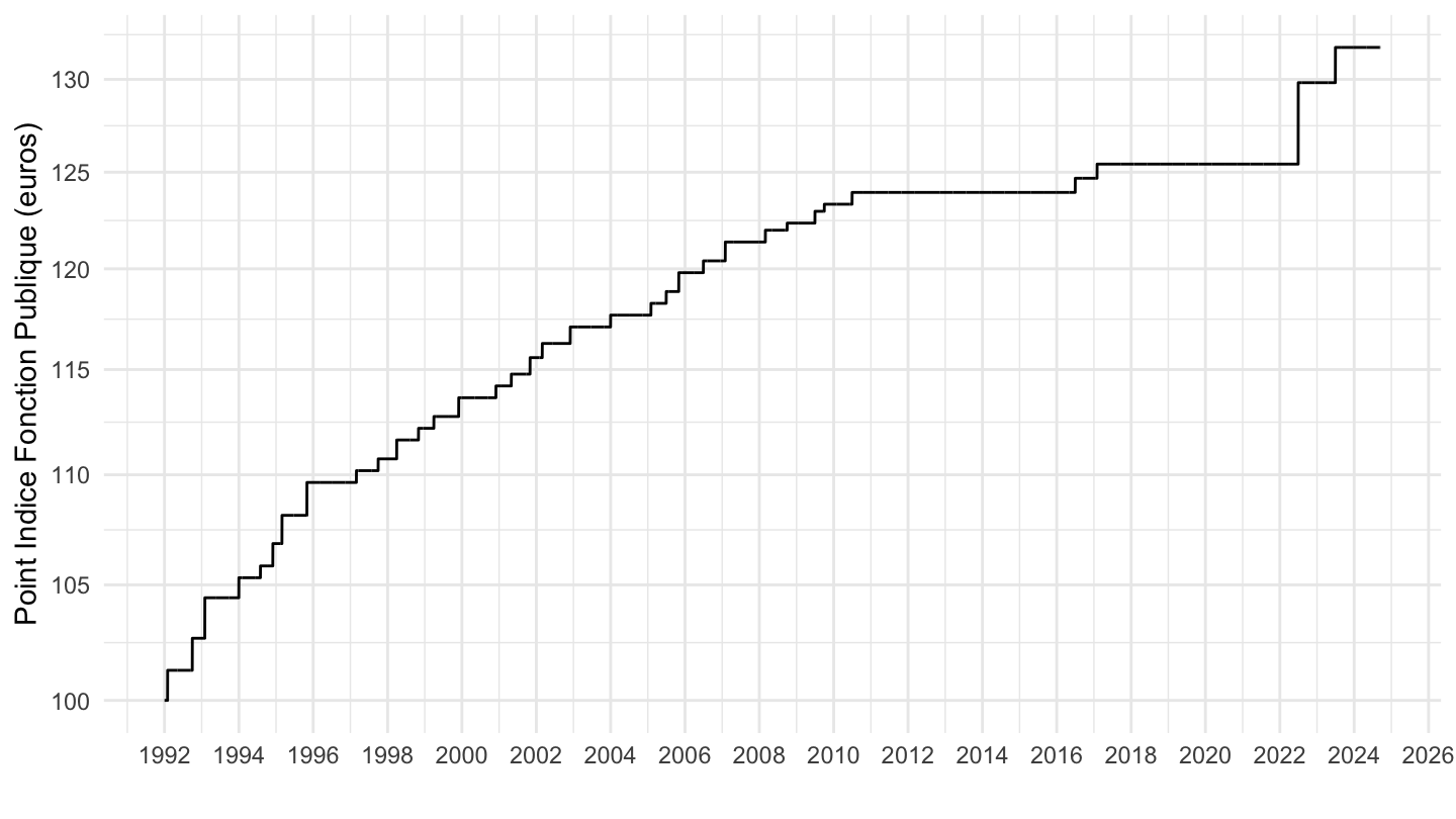
1996-
Valeur
Code
indicefp |>
  select(date, point_indice_en_euros) |>
  gather(variable, value, -date) |>
  group_by(variable) |>
  complete(date = seq.Date(min(date), max(date), by = "day")) |>
  fill(value) |>
  filter(date >= as.Date("1996-01-01")) |>
  ggplot() + geom_line(aes(x = date, y = value)) +
  theme_minimal() + ylab("Point Indice Fonction Publique (euros)") + xlab("") +
  scale_x_date(breaks = seq(1920, 2100, 2) |> paste0("-01-01") |> as.Date(),
               labels = date_format("%Y")) +
  scale_y_log10(breaks = seq(0, 200, 1),
                     labels = dollar_format(accuracy = 1, suffix = " € / point", prefix = ""))
Base 100
Code
indicefp |>
  select(date, point_indice_en_euros) |>
  gather(variable, value, -date) |>
  group_by(variable) |>
  complete(date = seq.Date(min(date), max(date), by = "day")) |>
  fill(value) |>
  filter(date >= as.Date("1996-01-01")) |>
  mutate(value = 100*value/value[1]) |>
  ggplot() + geom_line(aes(x = date, y = value)) +
  theme_minimal() + ylab("Point Indice Fonction Publique (euros)") + xlab("") +
  scale_x_date(breaks = seq(1920, 2100, 2) |> paste0("-01-01") |> as.Date(),
               labels = date_format("%Y")) +
  scale_y_log10(breaks = seq(0, 200, 5))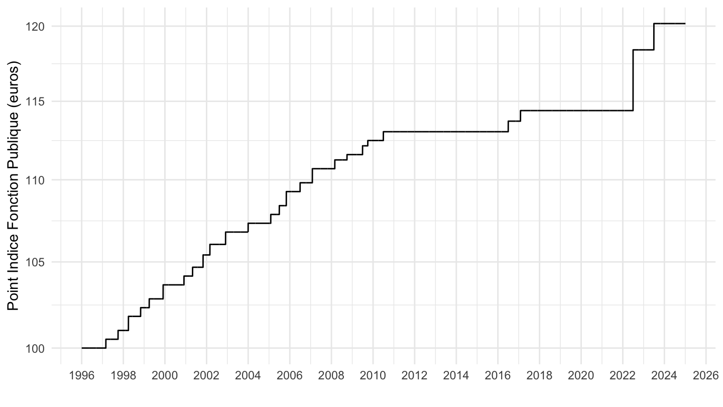
inflation
Table
Code
cpi |>
  print_table_conditional()
Graph
All
Code
cpi |>
  mutate(cpi = 100*cpi/cpi[date == as.Date("1951-01-01")]) |>
  ggplot() + geom_line(aes(x = date, y = cpi)) +
  scale_x_date(breaks = seq(1950, 2100, 5) |> paste0("-01-01") |> as.Date(),
               labels = date_format("%Y")) +
  scale_y_log10(breaks = c(100, 200, 300, 500, 800, 1000, 1200, 1500, 2000)) +
  theme_minimal() + xlab("") + ylab("")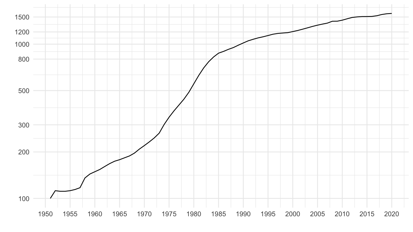
1990-
Code
cpi |>
  filter(date >= as.Date("1990-01-01")) |>
  mutate(cpi = 100*cpi/cpi[date == as.Date("1990-01-01")]) |>
  ggplot() + geom_line(aes(x = date, y = cpi)) +
  scale_x_date(breaks = seq(1950, 2100, 5) |> paste0("-01-01") |> as.Date(),
               labels = date_format("%Y")) +
  scale_y_log10(breaks = seq(100, 200, 5)) +
  theme_minimal() + xlab("") + ylab("Inflation (100 = 1990)")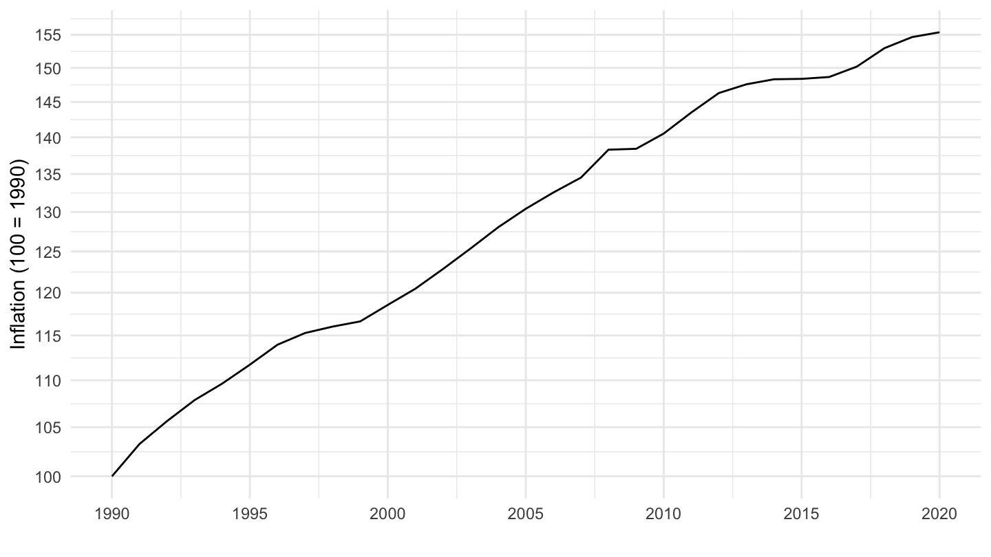
1995-
Code
cpi |>
  filter(date >= as.Date("1995-01-01")) |>
  mutate(cpi = 100*cpi/cpi[date == as.Date("1995-01-01")]) |>
  ggplot() + geom_line(aes(x = date, y = cpi)) +
  scale_x_date(breaks = seq(1950, 2100, 5) |> paste0("-01-01") |> as.Date(),
               labels = date_format("%Y")) +
  scale_y_log10(breaks = seq(100, 200, 5)) +
  theme_minimal() + xlab("") + ylab("Inflation (100 = 1995)")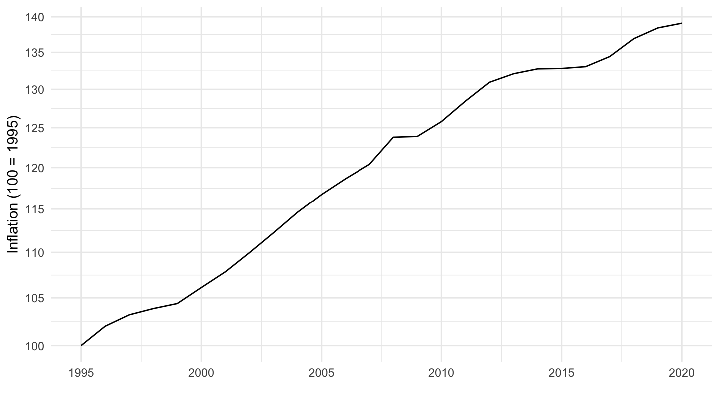
1996-
Code
cpi |>
  filter(date >= as.Date("1996-01-01")) |>
  mutate(cpi = 100*cpi/cpi[date == as.Date("1996-01-01")]) |>
  ggplot() + geom_line(aes(x = date, y = cpi)) +
  scale_x_date(breaks = seq(1950, 2100, 2) |> paste0("-01-01") |> as.Date(),
               labels = date_format("%Y")) +
  scale_y_log10(breaks = seq(100, 200, 5)) +
  theme_minimal() + xlab("") + ylab("Inflation (100 = 1996)")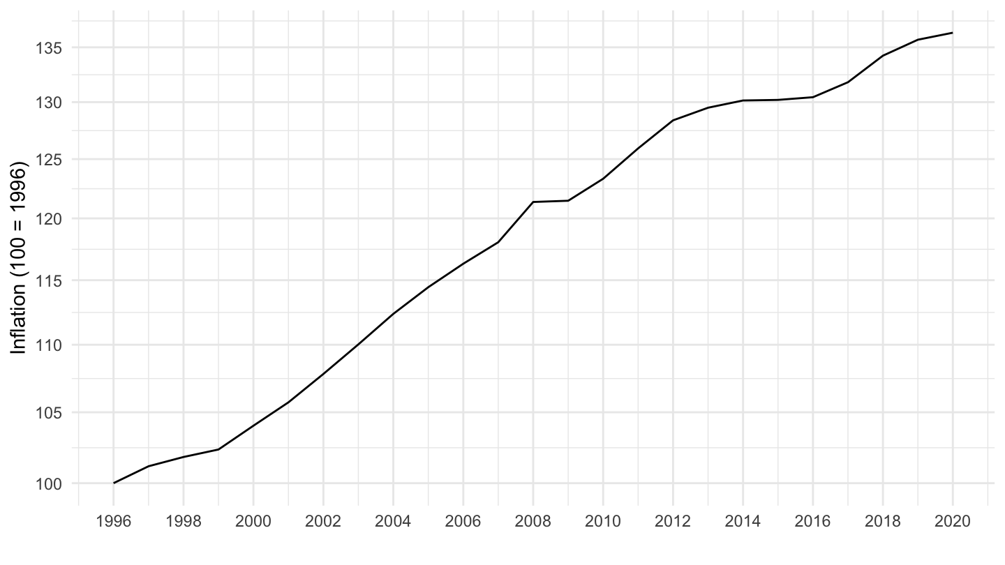
2000-
Code
cpi |>
  filter(date >= as.Date("2000-01-01")) |>
  mutate(cpi = 100*cpi/cpi[date == as.Date("2000-01-01")]) |>
  ggplot() + geom_line(aes(x = date, y = cpi)) +
  scale_x_date(breaks = seq(1950, 2100, 2) |> paste0("-01-01") |> as.Date(),
               labels = date_format("%Y")) +
  scale_y_log10(breaks = seq(100, 200, 5)) +
  theme_minimal() + xlab("") + ylab("Inflation (100 = 2000)")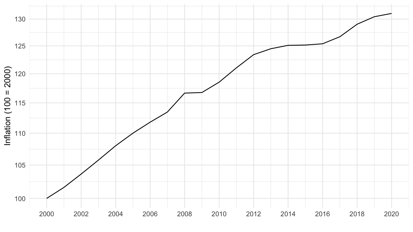
2012-
Code
cpi |>
  filter(date >= as.Date("2012-01-01")) |>
  mutate(cpi = 100*cpi/cpi[date == as.Date("2012-01-01")]) |>
  ggplot() + geom_line(aes(x = date, y = cpi)) +
  scale_x_date(breaks = seq(1950, 2100, 2) |> paste0("-01-01") |> as.Date(),
               labels = date_format("%Y")) +
  scale_y_log10(breaks = seq(100, 200, 1)) +
  theme_minimal() + xlab("") + ylab("Inflation (100 = 2012)")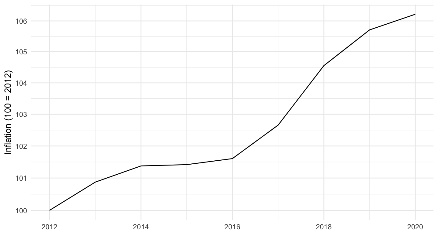
Indice Fonction Publique Réel
1970-
Annuel
Code
indicefp |>
  select(date, point_indice_en_euros) |>

  arrange(desc(date)) |>
  gather(variable, value, -date) |>
  group_by(variable) |>
  complete(date = seq.Date(min(date), max(date), by = "day")) |>
  fill(value) |>
  filter(month(date) == 1,
         day(date) == 1) |>
  left_join(cpi, by = "date") |>
  mutate(value = value/cpi,
         value = 100*value/value[1]) |>
  ggplot() + geom_line(aes(x = date, y = value)) + theme_minimal() +
  scale_x_date(breaks = seq(1920, 2100, 5) |> paste0("-01-01") |> as.Date(),
               labels = date_format("%Y")) +
  scale_y_log10(breaks = seq(0, 200, 2)) +
  ylab("Point Indice Fonction Publique (euros constants)") + xlab("")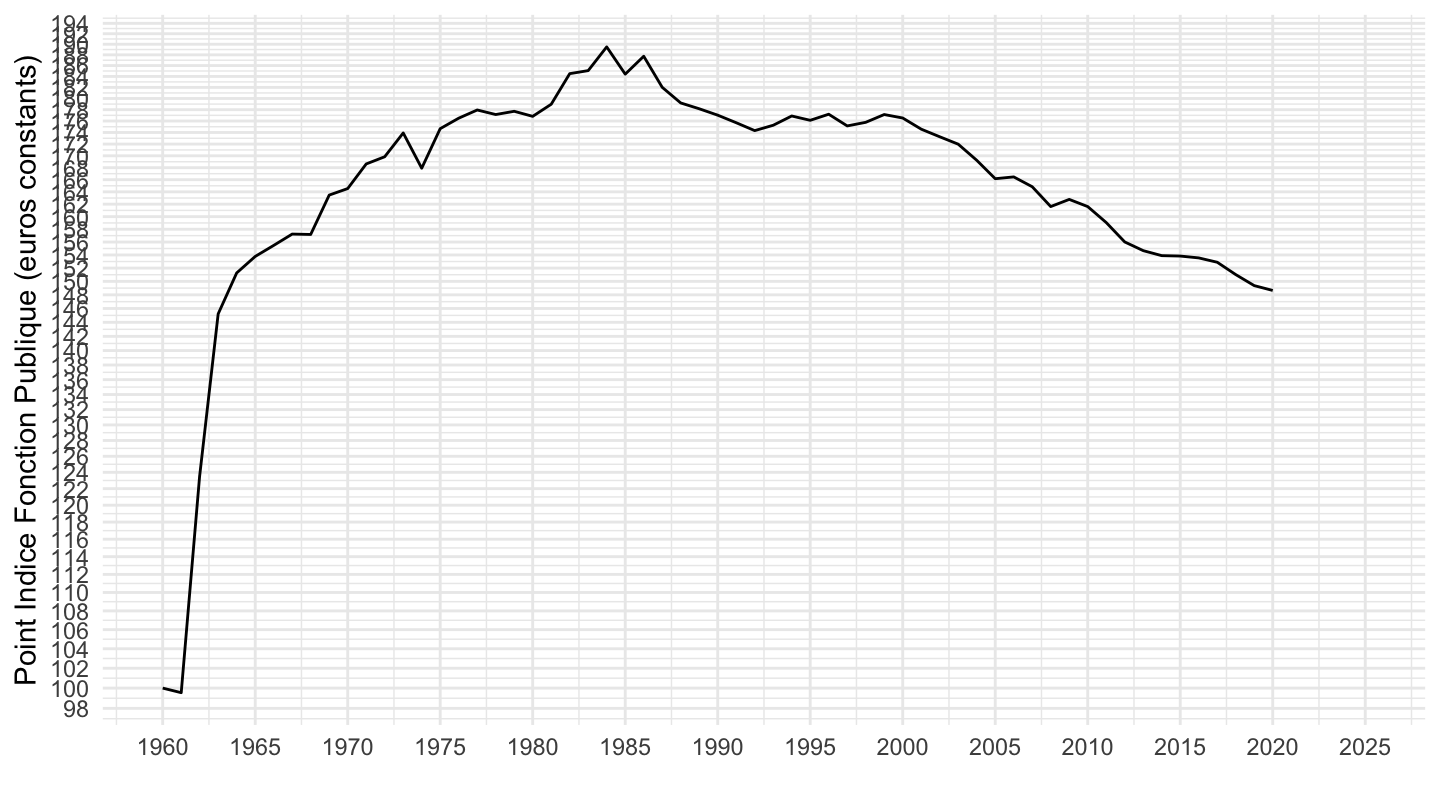
1965-
Annuel
Code
indicefp |>
  select(date, point_indice_en_euros) |>

  arrange(desc(date)) |>
  gather(variable, value, -date) |>
  group_by(variable) |>
  complete(date = seq.Date(min(date), max(date), by = "day")) |>
  fill(value) |>
  filter(date >= as.Date("1965-01-01")) |>
  filter(month(date) == 1,
         day(date) == 1) |>
  left_join(cpi, by = "date") |>
  mutate(value = value/cpi,
         value = 100*value/value[1]) |>
  ggplot() + geom_line(aes(x = date, y = value)) + theme_minimal() +
  scale_x_date(breaks = seq(1920, 2100, 5) |> paste0("-01-01") |> as.Date(),
               labels = date_format("%Y")) +
  scale_y_log10(breaks = seq(0, 200, 2)) +
  ylab("Point Indice Fonction Publique (euros constants)") + xlab("")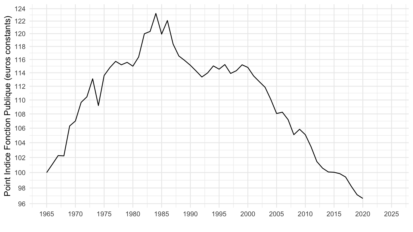
1996-
Annuel
Code
indicefp |>
  select(date, point_indice_en_euros) |>

  arrange(desc(date)) |>
  gather(variable, value, -date) |>
  group_by(variable) |>
  complete(date = seq.Date(min(date), max(date), by = "day")) |>
  fill(value) |>
  filter(month(date) == 1,
         day(date) == 1) |>
  left_join(cpi, by = "date") |>
  filter(date >= as.Date("1996-01-01")) |>
  mutate(value = value/cpi,
         value = 100*value/value[1]) |>
  ggplot() + geom_line(aes(x = date, y = value)) + theme_minimal() +
  scale_x_date(breaks = seq(1920, 2100, 2) |> paste0("-01-01") |> as.Date(),
               labels = date_format("%Y")) +
  scale_y_log10(breaks = seq(0, 200, 2)) +
  ylab("Point Indice Fonction Publique (euros constants)") + xlab("")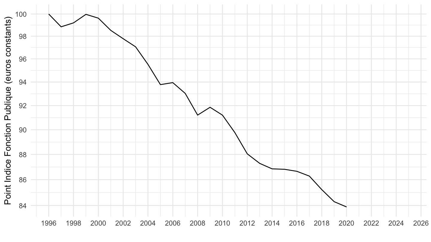
CPI
Code
indicefp |>
  select(date, point_indice_en_euros) |>

  arrange(desc(date)) |>
  gather(variable, value, -date) |>
  group_by(variable) |>
  complete(date = seq.Date(min(date), max(date), by = "day")) |>
  fill(value) |>
  filter(month(date) == 1,
         day(date) == 1) |>
  left_join(cpi2, by = "date") |>
  filter(date >= as.Date("1996-01-01")) |>
  mutate(value = value/cpi,
         value = 100*value/value[1]) |>
  ggplot() + geom_line(aes(x = date, y = value)) + theme_minimal() +
  scale_x_date(breaks = seq(1920, 2100, 2) |> paste0("-01-01") |> as.Date(),
               labels = date_format("%Y")) +
  scale_y_log10(breaks = seq(0, 200, 2)) +
  ylab("Point Indice Fonction Publique (€ constants)") + xlab("")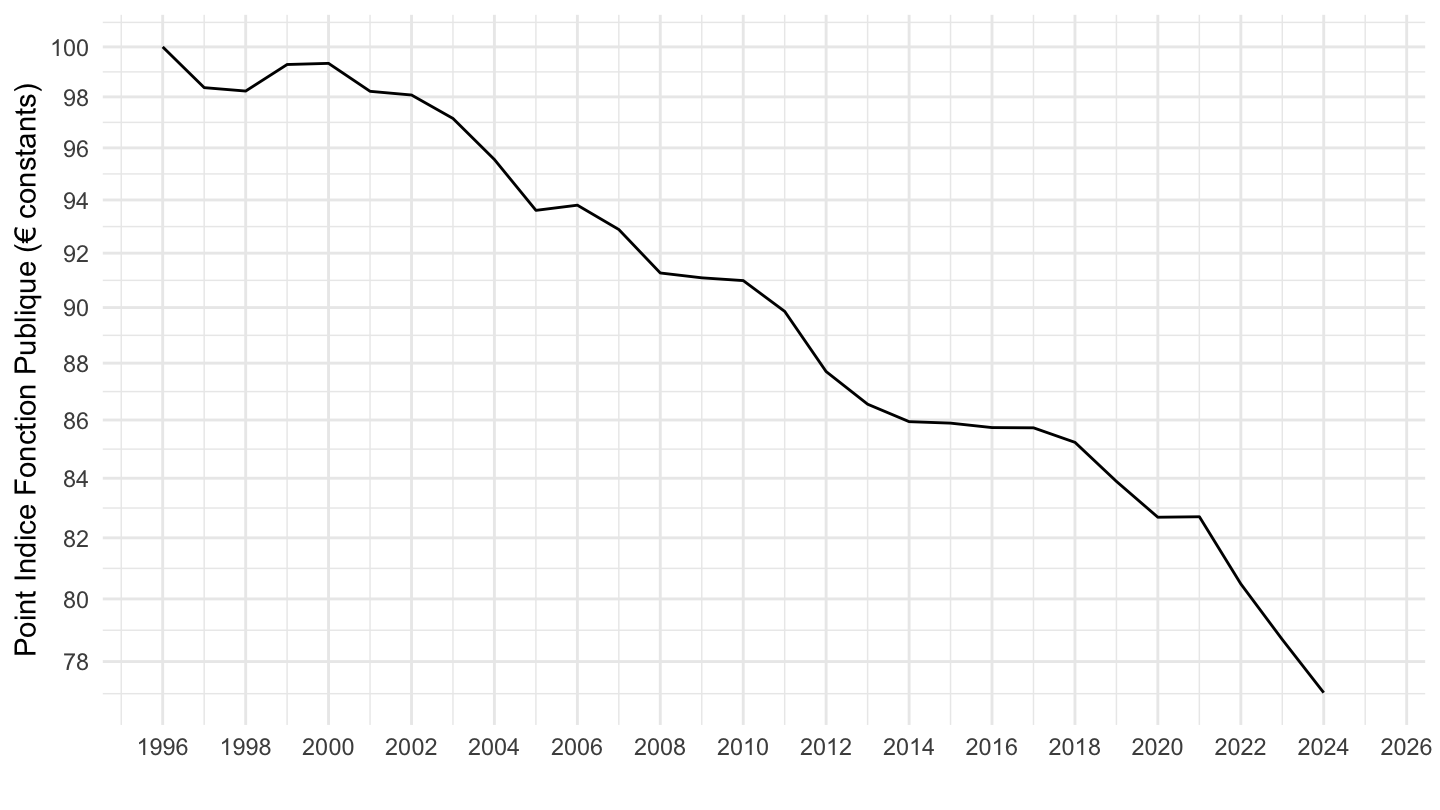
CPIH
All
Code
indicefp |>
  select(date, point_indice_en_euros) |>
  arrange(desc(date)) |>
  gather(variable, value, -date) |>
  group_by(variable) |>
  complete(date = seq.Date(min(date), max(date), by = "day")) |>
  fill(value) |>
  filter(month(date) == 1,
         day(date) == 1) |>
  left_join(cpi2, by = "date") |>
  filter(date >= as.Date("1997-01-01")) |>
  mutate(value = value/cpih,
         value = 100*value/value[1]) |>
  ggplot() + geom_line(aes(x = date, y = value)) + theme_minimal() +
  scale_x_date(breaks = seq(1920, 2100, 2) |> paste0("-01-01") |> as.Date(),
               labels = date_format("%Y")) +
  scale_y_log10(breaks = seq(0, 200, 2)) +
  ylab("Point Indice Fonction Publique (€ constants)") + xlab("")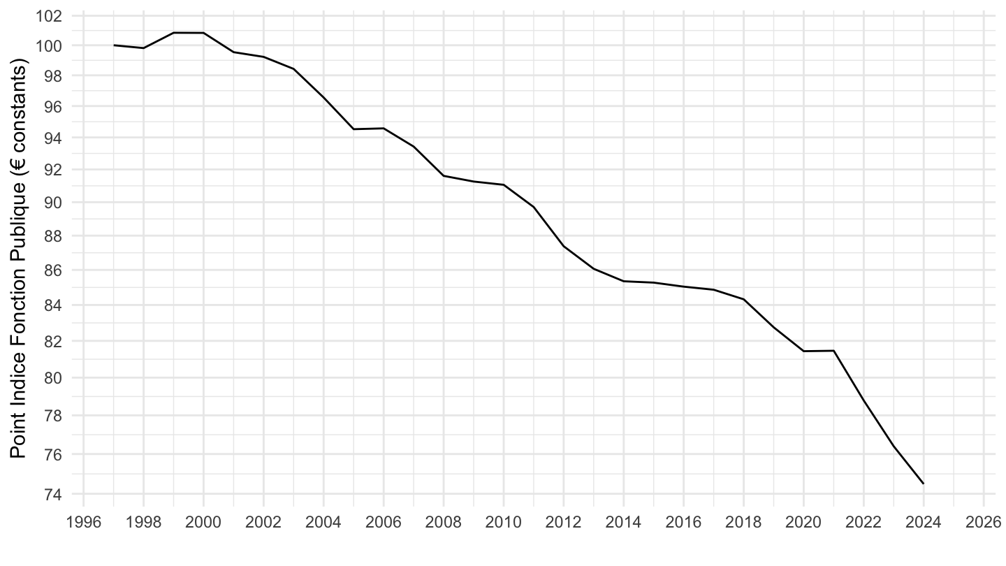
in %
Code
data_alter_eco <- indicefp |>
  select(date, point_indice_en_euros) |>
  gather(variable, value, -date) |>
  group_by(variable) |>
  complete(date = seq.Date(min(date), max(date), by = "day")) |>
  fill(value) |>
  ungroup() |>
  filter(month(date) == 1,
         day(date) == 1) |>
  left_join(cpi2, by = "date") |>
  filter(date >= as.Date("1996-01-01")) |>
  transmute(date,
            value_cpih = value/cpih,
            value_cpi = value/cpi) |>
  transmute(date,
            `Valeur du Point d'Indice de la Fonction Publique par rapport à 1996 (IPCH, Eurostat)` = value_cpih/value_cpih[1],
            `Valeur du Point d'Indice de la Fonction Publique par rapport à 1996 (IPC, INSEE)` = value_cpi/value_cpi[1])

write_csv(data_alter_eco, file = "data_alter_eco.csv")

data_alter_eco |>
  gather(variable, value, -date) |>
  ggplot() + geom_line(aes(x = date, y = value, color = variable)) + theme_minimal() +
  scale_x_date(breaks = seq(1920, 2100, 2) |> paste0("-01-01") |> as.Date(),
               labels = date_format("%Y")) +
  scale_color_manual(values = viridis(3)[1:2]) +
  theme(legend.position = c(0.43, 0.1),
        legend.title = element_blank()) +
  scale_y_log10(breaks = seq(1, 0.02, -0.02),
                labels = percent(seq(1, 0.02, -0.02)-1, acc = 1)) +
  ylab("Valeur du Point Indice Fonction Publique vs. 1996") + xlab("")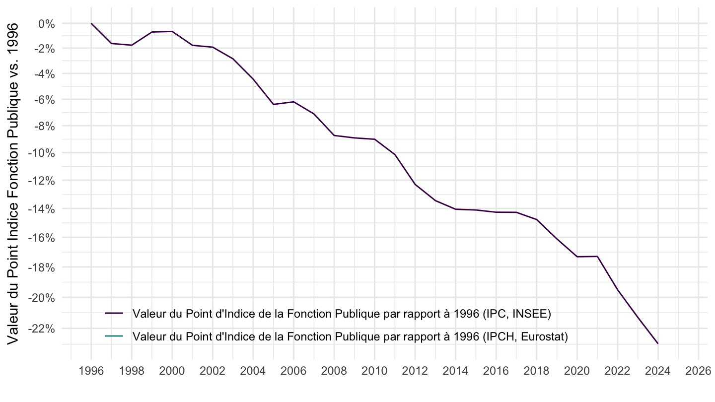
in %
Code
indicefp |>
  select(date, point_indice_en_euros) |>
  gather(variable, value, -date) |>
  group_by(variable) |>
  complete(date = seq.Date(min(date), max(date), by = "day")) |>
  fill(value) |>
  ungroup() |>
  filter(month(date) == 1,
         day(date) == 1) |>
  left_join(cpi2, by = "date") |>
  filter(date >= as.Date("1997-01-01")) |>
  transmute(date,
            value_cpih = value/cpih,
            value_cpi = value/cpi) |>
  transmute(date,
            `Valeur réelle du Point d'Indice par rapport à 1996` = value_cpih/value_cpih[1]) |>
  gather(variable, value, -date) |>
  ggplot() + geom_line(aes(x = date, y = value)) + theme_minimal() +
  scale_x_date(breaks = seq(1920, 2100, 2) |> paste0("-01-01") |> as.Date(),
               labels = date_format("%Y")) +
  scale_color_manual(values = viridis(3)[1:2]) +
  theme(legend.position = c(0.43, 0.1),
        legend.title = element_blank()) +
  scale_y_log10(breaks = seq(1, 0.02, -0.02),
                labels = percent(seq(1, 0.02, -0.02)-1, acc = 1)) +
  ylab("Valeur du Point Indice vs. 1996") + xlab("") +
  labs(title = "Valeur réelle du Point Indice de la Fonction Publique par rapport à 1997",
              subtitle = "(Indice des prix utilisé: Indice des Prix à la Consommation Harmonisé (IPCH))")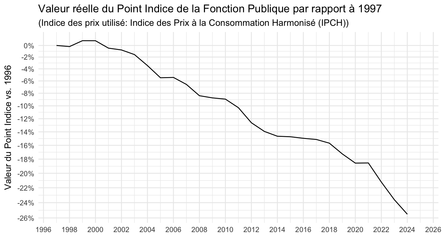
1996-
1997-
Mensuel
Code
net_brut_mensuel <- read_parquet(here::here("data", "insee", "INDICE-TRAITEMENT-FP-net-brut-mensuel.parquet"))
indicefp |>
  select(date, point_indice_en_euros) |>
  arrange(desc(date)) |>
  gather(variable, value, -date) |>
  group_by(variable) |>
  complete(date = seq.Date(min(date), max(date), by = "day")) |>
  fill(value) |>
  ungroup() |>
  left_join(cpi2_m, by = "date") |>
  filter(day(date) == 1) |>
  left_join(net_brut_mensuel, by = "date") |>
  filter(date >= as.Date("1997-01-01")) |>
  transmute(date,
            `Valeur du Point d'Indice de la Fonction Publique vs. 1997 (IPCH, Eurostat)` = (value/value[1])*(cpih[1]/cpih)*net_brut,
            `Valeur du Point d'Indice de la Fonction Publique vs. 1997 (IPC, INSEE)` = (value/value[1])*(cpi[1]/cpi)*net_brut) |>
  gather(variable, OBS_VALUE, -date) |>
  ggplot() + geom_line(aes(x = date, y = OBS_VALUE, color = variable)) + theme_minimal() +
  scale_x_date(breaks = c(seq(1997, 2100, 5), seq(1999, 2100, 5)) |> paste0("-01-01") |> as.Date(),
               labels = date_format("%Y")) +
  theme(legend.position = c(0.43, 0.12),
        legend.title = element_blank()) +
  scale_y_log10(breaks = seq(1, 0.02, -0.02),
                labels = percent(seq(1, 0.02, -0.02)-1, acc = 1)) +
  ylab("Valeur du Point Indice Fonction Publique vs. 1997") + xlab("") +
  geom_text(data = . %>% filter((year(date) %in% seq(1999, 2019, 5) & month(date) == 1) | date == max(date)),
            aes(x = date, y = OBS_VALUE, label = percent(OBS_VALUE-1, acc = 0.1)),
                  fontface ="bold", color = "black", size = 3)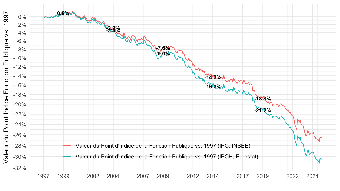
1999-
Code
indicefp |>
  select(date, point_indice_en_euros) |>
  gather(variable, value, -date) |>
  group_by(variable) |>
  complete(date = seq.Date(min(date), max(date), by = "day")) |>
  fill(value) |>
  ungroup() |>
  filter(month(date) == 1,
         day(date) == 1) |>
  left_join(cpi2, by = "date") |>
  filter(date >= as.Date("1999-01-01")) |>
  transmute(date,
            value_cpih = value/cpih,
            value_cpi = value/cpi) |>
  transmute(date,
            `Valeur du Point d'Indice de la Fonction Publique vs. 1999 (IPCH, Eurostat)` = value_cpih/value_cpih[1]-1,
            `Valeur du Point d'Indice de la Fonction Publique vs. 1999 (IPC, INSEE)` = value_cpi/value_cpi[1]-1) |>
  gather(variable, OBS_VALUE, -date) |>
  ggplot() + geom_line(aes(x = date, y = OBS_VALUE, color = variable)) + theme_minimal() +
  scale_x_date(breaks = seq(1999, 2100, 5) |> paste0("-01-01") |> as.Date(),
               labels = date_format("%Y")) +
  theme(legend.position = c(0.43, 0.12),
        legend.title = element_blank()) +
  scale_y_continuous(breaks = 0.01*seq(-200, 200, 2),
                     labels = percent_format(acc = 1)) +
  ylab("Valeur du Point Indice Fonction Publique vs. 1999") + xlab("") +
  geom_text(data = . %>% filter(year(date) %in% seq(1999, 2040, 5)),aes(x = date, y = OBS_VALUE, label = percent(OBS_VALUE, acc = 0.1)),
                  fontface ="plain", color = "black", size = 3)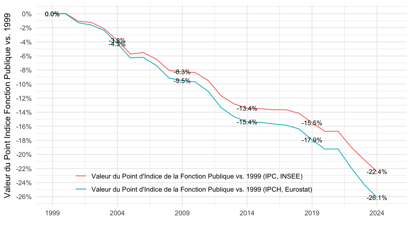
2015- (avec correction net brut)
Annuel
Code
net_brut_annuel <- read_parquet(here::here("data", "insee", "INDICE-TRAITEMENT-FP-net-brut-annuel.parquet"))
indicefp |>
  select(date, point_indice_en_euros) |>
  arrange(desc(date)) |>
  gather(variable, value, -date) |>
  group_by(variable) |>
  complete(date = seq.Date(min(date), max(date), by = "day")) |>
  fill(value) |>
  ungroup() |>
  filter(month(date) == 1,
         day(date) == 1) |>
  left_join(cpi2, by = "date") |>
  left_join(net_brut_annuel, by = "date") |>
  filter(date >= as.Date("2015-01-01")) |>
  transmute(date,
            `Valeur du Point d'Indice de la Fonction Publique vs. 1999 (IPCH, Eurostat)` = (value/value[1])*(cpih[1]/cpih)*net_brut-1,
            `Valeur du Point d'Indice de la Fonction Publique vs. 1999 (IPC, INSEE)` = (value/value[1])*(cpi[1]/cpi)*net_brut-1) |>
  gather(variable, OBS_VALUE, -date) |>
  ggplot() + geom_line(aes(x = date, y = OBS_VALUE, color = variable)) + theme_minimal() +
  scale_x_date(breaks = seq(1999, 2100, 5) |> paste0("-01-01") |> as.Date(),
               labels = date_format("%Y")) +
  theme(legend.position = c(0.43, 0.12),
        legend.title = element_blank()) +
  scale_y_continuous(breaks = 0.01*seq(-200, 200, 2),
                     labels = percent_format(acc = 1)) +
  ylab("Valeur du Point Indice Fonction Publique vs. 1999") + xlab("") +
  geom_text(data = . %>% filter(year(date) %in% seq(1999, 2040, 5)),
            aes(x = date, y = OBS_VALUE, label = percent(OBS_VALUE, acc = 1)),
                  fontface ="plain", color = "black", size = 3)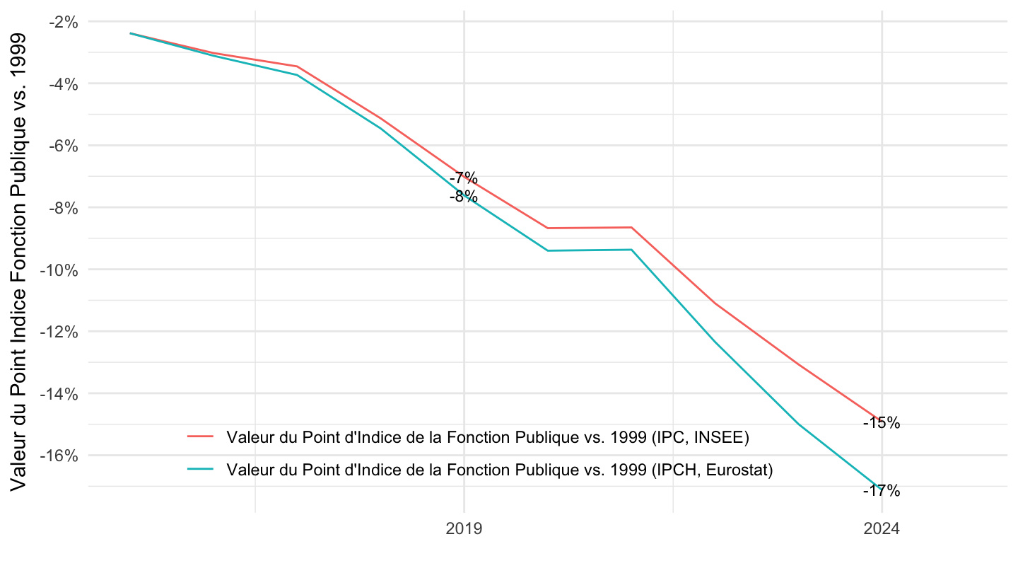
Mensuel
Code
net_brut_mensuel <- read_parquet(here::here("data", "insee", "INDICE-TRAITEMENT-FP-net-brut-mensuel.parquet"))
indicefp |>
  select(date, point_indice_en_euros) |>
  arrange(desc(date)) |>
  gather(variable, value, -date) |>
  group_by(variable) |>
  complete(date = seq.Date(min(date), max(date), by = "day")) |>
  fill(value) |>
  ungroup() |>
  left_join(cpi2_m, by = "date") |>
  filter(day(date) == 1) |>
  left_join(net_brut_mensuel, by = "date") |>
  filter(date >= as.Date("2015-01-01")) |>
  transmute(date,
            `Valeur du Point d'Indice de la Fonction Publique vs. 2015 (IPCH, Eurostat)` = (value/value[1])*(cpih[1]/cpih)*(net_brut/net_brut[1]),
            `Valeur du Point d'Indice de la Fonction Publique vs. 2015 (IPC, INSEE)` = (value/value[1])*(cpi[1]/cpi)*(net_brut/net_brut[1])) |>
  gather(variable, OBS_VALUE, -date) |>
  ggplot() + geom_line(aes(x = date, y = OBS_VALUE, color = variable)) + theme_minimal() +
  scale_x_date(breaks = c(seq(1999, 2100, 1), seq(1997, 2100, 5)) |> paste0("-01-01") |> as.Date(),
               labels = date_format("%Y")) +
  theme(legend.position = c(0.43, 0.12),
        legend.title = element_blank()) +
  scale_y_log10(breaks = seq(1, 0.02, -0.02),
                labels = percent(seq(1, 0.02, -0.02)-1, acc = 1)) +
  ylab("Valeur du Point Indice Fonction Publique vs. 2015") + xlab("") +
  geom_label(data = . %>% filter(date == max(date)),
            aes(x = date, y = OBS_VALUE, label = percent(OBS_VALUE-1, acc = 0.1), color = variable),
                  fontface ="bold", size = 4)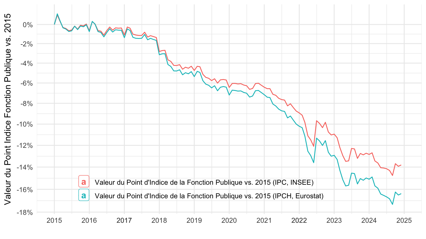
2021T2-
Code
invisible(Sys.setlocale("LC_TIME", "fr_FR.UTF-8"))
net_brut_mensuel <- read_parquet(here::here("data", "insee", "INDICE-TRAITEMENT-FP-net-brut-mensuel.parquet"))
indicefp |>
  select(date, point_indice_en_euros) |>
  arrange(desc(date)) |>
  gather(variable, value, -date) |>
  group_by(variable) |>
  complete(date = seq.Date(min(date), max(date), by = "day")) |>
  fill(value) |>
  ungroup() |>
  left_join(cpi2_m, by = "date") |>
  filter(day(date) == 1) |>
  left_join(net_brut_mensuel, by = "date") |>
  filter(date >= as.Date("2021-04-01")) |>
  transmute(date,
            `Valeur du Point d'Indice de la Fonction Publique vs. Avril 2021 (IPCH, Eurostat)` = (value/value[1])*(cpih[1]/cpih)*(net_brut/net_brut[1]),
            `Valeur du Point d'Indice de la Fonction Publique vs. Avril 2021 (IPC, INSEE)` = (value/value[1])*(cpi[1]/cpi)*(net_brut/net_brut[1])) |>
  gather(variable, OBS_VALUE, -date) |>
  filter(!is.na(OBS_VALUE)) |>
  ggplot() + geom_line(aes(x = date, y = OBS_VALUE, color = variable)) + theme_minimal() +
  scale_x_date(breaks = "3 months",
               labels = date_format("%B %Y")) +
  theme(legend.position = c(0.43, 0.12),
        legend.title = element_blank(),
        axis.text.x = element_text(angle = 45, vjust = 1, hjust = 1)) +
  scale_y_log10(breaks = seq(1, 0.02, -0.01),
                labels = percent(seq(1, 0.02, -0.01)-1, acc = 1)) +
  ylab("Valeur du Point Indice Fonction Publique vs. Avril 2021") + xlab("") +
  geom_label(data = . %>% filter(date == max(date)),
            aes(x = date, y = OBS_VALUE, label = percent(OBS_VALUE-1, acc = 0.1), color = variable),
                  fontface ="bold")
2021T4-
Code
net_brut_mensuel <- read_parquet(here::here("data", "insee", "INDICE-TRAITEMENT-FP-net-brut-mensuel.parquet"))
indicefp |>
  select(date, point_indice_en_euros) |>
  arrange(desc(date)) |>
  gather(variable, value, -date) |>
  group_by(variable) |>
  complete(date = seq.Date(min(date), max(date), by = "day")) |>
  fill(value) |>
  ungroup() |>
  left_join(cpi2_m, by = "date") |>
  filter(day(date) == 1) |>
  left_join(net_brut_mensuel, by = "date") |>
  filter(date >= as.Date("2021-10-01")) |>
  transmute(date,
            `Valeur du Point d'Indice de la Fonction Publique vs. 2021T4 (IPCH, Eurostat)` = (value/value[1])*(cpih[1]/cpih)*(net_brut/net_brut[1]),
            `Valeur du Point d'Indice de la Fonction Publique vs. 2015 (IPC, INSEE)` = (value/value[1])*(cpi[1]/cpi)*(net_brut/net_brut[1])) |>
  gather(variable, OBS_VALUE, -date) |>
  ggplot() + geom_line(aes(x = date, y = OBS_VALUE, color = variable)) + theme_minimal() +
  scale_x_date(breaks = "3 months",
               labels = date_format("%Y %b")) +
  theme(legend.position = c(0.43, 0.12),
        legend.title = element_blank(),
        axis.text.x = element_text(angle = 45, vjust = 1, hjust = 1)) +
  scale_y_log10(breaks = seq(1, 0.02, -0.01),
                labels = percent(seq(1, 0.02, -0.01)-1, acc = 1)) +
  ylab("Valeur du Point Indice Fonction Publique vs. 2015") + xlab("") +
  geom_label(data = . %>% filter(date == max(date)),
            aes(x = date, y = OBS_VALUE, label = percent(OBS_VALUE-1, acc = 0.1)),
                  fontface ="bold", color = "black", size = 3)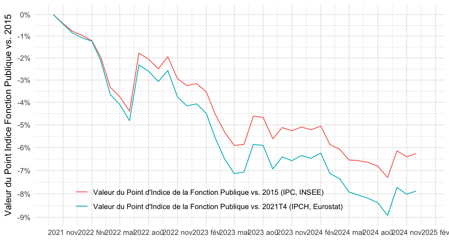
2012-
Mensuel
Code
net_brut_mensuel <- read_parquet(here::here("data", "insee", "INDICE-TRAITEMENT-FP-net-brut-mensuel.parquet"))
indicefp |>
  select(date, point_indice_en_euros) |>
  arrange(desc(date)) |>
  gather(variable, value, -date) |>
  group_by(variable) |>
  complete(date = seq.Date(min(date), max(date), by = "day")) |>
  fill(value) |>
  ungroup() |>
  left_join(cpi2_m, by = "date") |>
  filter(day(date) == 1) |>
  left_join(net_brut_mensuel, by = "date") |>
  filter(date >= as.Date("2012-01-01")) |>
  transmute(date,
            `Valeur du Point d'Indice de la Fonction Publique vs. 2012 (IPCH, Eurostat)` = (value/value[1])*(cpih[1]/cpih)*(net_brut/net_brut[1]),
            `Valeur du Point d'Indice de la Fonction Publique vs. 2012 (IPC, INSEE)` = (value/value[1])*(cpi[1]/cpi)*(net_brut/net_brut[1])) |>
  gather(variable, OBS_VALUE, -date) |>
  ggplot() + geom_line(aes(x = date, y = OBS_VALUE, color = variable)) + theme_minimal() +
  scale_x_date(breaks = c(seq(1999, 2100, 1), seq(1997, 2100, 5)) |> paste0("-01-01") |> as.Date(),
               labels = date_format("%Y")) +
  theme(legend.position = c(0.43, 0.12),
        legend.title = element_blank()) +
  scale_y_log10(breaks = seq(1, 0.02, -0.02),
                labels = percent(seq(1, 0.02, -0.02)-1, acc = 1)) +
  ylab("Valeur du Point Indice Fonction Publique vs. 2012") + xlab("") +
  geom_text_repel(data = . %>% filter(year(date) %in% c(2017, 2024),
                                month(date) == 3),
            aes(x = date, y = OBS_VALUE, label = percent(OBS_VALUE-1, acc = 0.1)),
                  fontface ="bold", color = "black", size = 3)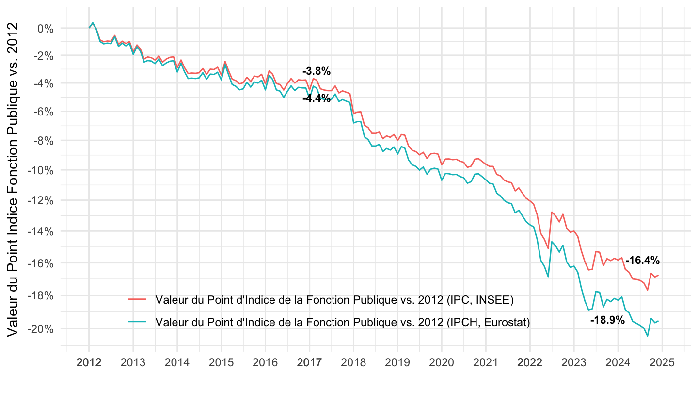
1999- (avec correction net brut)
Annuel
Code
net_brut_annuel <- read_parquet(here::here("data", "insee", "INDICE-TRAITEMENT-FP-net-brut-annuel.parquet"))
indicefp |>
  select(date, point_indice_en_euros) |>
  arrange(desc(date)) |>
  gather(variable, value, -date) |>
  group_by(variable) |>
  complete(date = seq.Date(min(date), max(date), by = "day")) |>
  fill(value) |>
  ungroup() |>
  filter(month(date) == 1,
         day(date) == 1) |>
  left_join(cpi2, by = "date") |>
  left_join(net_brut_annuel, by = "date") |>
  filter(date >= as.Date("1999-01-01")) |>
  transmute(date,
            `Valeur du Point d'Indice de la Fonction Publique vs. 1999 (IPCH, Eurostat)` = (value/value[1])*(cpih[1]/cpih)*net_brut-1,
            `Valeur du Point d'Indice de la Fonction Publique vs. 1999 (IPC, INSEE)` = (value/value[1])*(cpi[1]/cpi)*net_brut-1) |>
  gather(variable, OBS_VALUE, -date) |>
  ggplot() + geom_line(aes(x = date, y = OBS_VALUE, color = variable)) + theme_minimal() +
  scale_x_date(breaks = seq(1999, 2100, 5) |> paste0("-01-01") |> as.Date(),
               labels = date_format("%Y")) +
  theme(legend.position = c(0.43, 0.12),
        legend.title = element_blank()) +
  scale_y_continuous(breaks = 0.01*seq(-200, 200, 2),
                     labels = percent_format(acc = 1)) +
  ylab("Valeur du Point Indice Fonction Publique vs. 1999") + xlab("") +
  geom_text(data = . %>% filter(year(date) %in% seq(1999, 2040, 5)),
            aes(x = date, y = OBS_VALUE, label = percent(OBS_VALUE, acc = 1)),
                  fontface ="plain", color = "black", size = 3)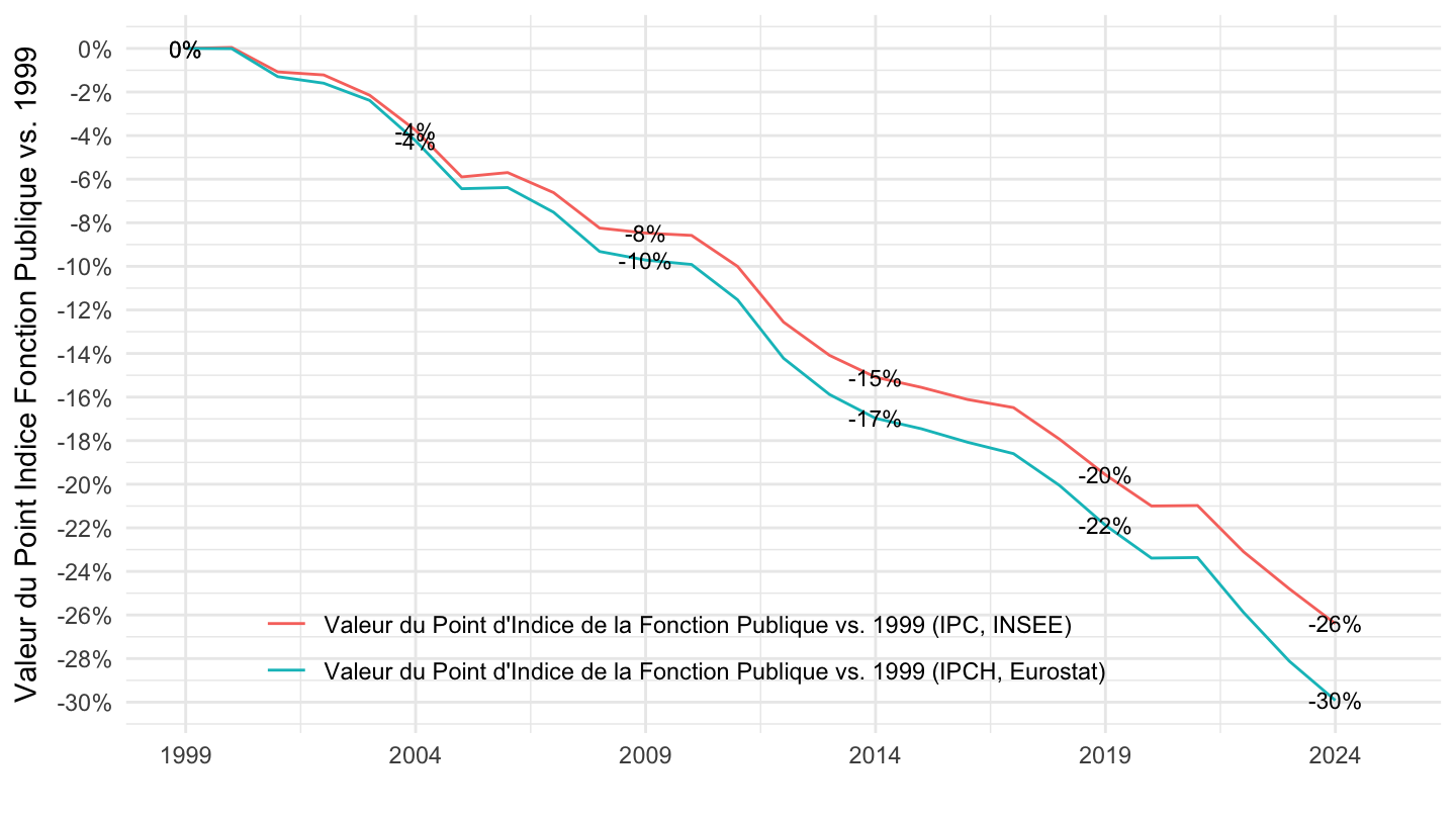
Trimestriel
Code
net_brut_trimestriel <- read_parquet(here::here("data", "insee", "INDICE-TRAITEMENT-FP-net-brut-trimestriel.parquet"))
indicefp |>
  select(date, point_indice_en_euros) |>
  arrange(desc(date)) |>
  gather(variable, value, -date) |>
  group_by(variable) |>
  complete(date = seq.Date(min(date), max(date), by = "day")) |>
  fill(value) |>
  ungroup() |>
  left_join(cpi2_m, by = "date") |>
  filter(month(date) %in% c(1, 4, 7, 10),
         day(date) == 1) |>
  left_join(net_brut_trimestriel, by = "date") |>
  filter(date >= as.Date("1999-01-01")) |>
  transmute(date,
            `Valeur du Point d'Indice de la Fonction Publique vs. 1999 (IPCH, Eurostat)` = (value/value[1])*(cpih[1]/cpih)*net_brut-1,
            `Valeur du Point d'Indice de la Fonction Publique vs. 1999 (IPC, INSEE)` = (value/value[1])*(cpi[1]/cpi)*net_brut-1) |>
  gather(variable, OBS_VALUE, -date) |>
  ggplot() + geom_line(aes(x = date, y = OBS_VALUE, color = variable)) + theme_minimal() +
  scale_x_date(breaks = seq(1999, 2100, 5) |> paste0("-01-01") |> as.Date(),
               labels = date_format("%Y")) +
  theme(legend.position = c(0.43, 0.12),
        legend.title = element_blank()) +
  scale_y_continuous(breaks = 0.01*seq(-200, 200, 2),
                     labels = percent_format(acc = 1)) +
  ylab("Valeur du Point Indice Fonction Publique vs. 1999") + xlab("") +
  geom_text(data = . %>% filter(year(date) %in% seq(1999, 2040, 5),
                                month(date) == 1),
            aes(x = date, y = OBS_VALUE, label = percent(OBS_VALUE, acc = 1)),
                  fontface ="plain", color = "black", size = 3)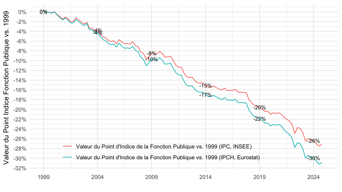
Mensuel
Code
net_brut_mensuel <- read_parquet(here::here("data", "insee", "INDICE-TRAITEMENT-FP-net-brut-mensuel.parquet"))
indicefp |>
  select(date, point_indice_en_euros) |>
  arrange(desc(date)) |>
  gather(variable, value, -date) |>
  group_by(variable) |>
  complete(date = seq.Date(min(date), max(date), by = "day")) |>
  fill(value) |>
  ungroup() |>
  left_join(cpi2_m, by = "date") |>
  filter(day(date) == 1) |>
  left_join(net_brut_mensuel, by = "date") |>
  filter(date >= as.Date("1999-01-01")) |>
  transmute(date,
            `Valeur du Point d'Indice de la Fonction Publique vs. 1999 (IPCH, Eurostat)` = (value/value[1])*(cpih[1]/cpih)*net_brut,
            `Valeur du Point d'Indice de la Fonction Publique vs. 1999 (IPC, INSEE)` = (value/value[1])*(cpi[1]/cpi)*net_brut) |>
  gather(variable, OBS_VALUE, -date) |>
  group_by(date) |>
  arrange(desc(date)) |>
  filter(!is.na(OBS_VALUE)) |>
  filter(n() == 2) |>
  ungroup() |>
  ggplot() + geom_line(aes(x = date, y = OBS_VALUE, color = variable)) + theme_minimal() +
  scale_x_date(breaks = c(seq(1999, 2100, 2)) |> paste0("-01-01") |> as.Date(),
               labels = date_format("%Y")) +
  theme(legend.position = c(0.43, 0.12),
        legend.title = element_blank()) +
  scale_y_log10(breaks = seq(1, 0.02, -0.02),
                labels = percent(seq(1, 0.02, -0.02)-1, acc = 1)) +
  ylab("Valeur du Point Indice Fonction Publique vs. 1999") + xlab("") +
  geom_text(data = . %>% filter((year(date) %in% seq(2009, 2019, 5) & month(date) == 1)),
            aes(x = date, y = OBS_VALUE, label = percent(OBS_VALUE-1, acc = 0.1)),
                  fontface ="bold", color = "black", size = 3) +
  geom_label(data = . %>% filter(date == max(date)),
            aes(x = date, y = OBS_VALUE, label = percent(OBS_VALUE-1, acc = 0.1), color = variable),
                  fontface ="bold", size = 3)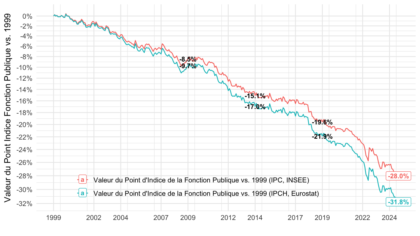
Mai 2007 (Sarkozy)
Code
net_brut_mensuel <- read_parquet(here::here("data", "insee", "INDICE-TRAITEMENT-FP-net-brut-mensuel.parquet"))
indicefp |>
  select(date, point_indice_en_euros) |>
  arrange(desc(date)) |>
  gather(variable, value, -date) |>
  group_by(variable) |>
  complete(date = seq.Date(min(date), max(date), by = "day")) |>
  fill(value) |>
  ungroup() |>
  left_join(cpi2_m, by = "date") |>
  filter(day(date) == 1) |>
  left_join(net_brut_mensuel, by = "date") |>
  filter(date >= as.Date("2007-05-01")) |>
  transmute(date,
            `Valeur du Point d'Indice de la Fonction Publique vs. mai 2007 (IPCH, Eurostat)` = (value/value[1])*(cpih[1]/cpih)*(net_brut/net_brut[1]),
            `Valeur du Point d'Indice de la Fonction Publique vs. mai 2007 (IPC, INSEE)` = (value/value[1])*(cpi[1]/cpi)*(net_brut/net_brut[1])) |>
  gather(variable, OBS_VALUE, -date) |>
  ggplot() + geom_line(aes(x = date, y = OBS_VALUE, color = variable)) + theme_minimal() +
  scale_x_date(breaks = c(seq(1999, 2100, 5), seq(1997, 2100, 5)) |> paste0("-01-01") |> as.Date(),
               labels = date_format("%Y")) +
  theme(legend.position = c(0.43, 0.12),
        legend.title = element_blank()) +
  scale_y_log10(breaks = seq(1, 0.02, -0.02),
                labels = percent(seq(1, 0.02, -0.02)-1, acc = 1)) +
  ylab("Valeur du Point Indice Net vs. mai 2007") + xlab("") +
  geom_text(data = . %>% filter(date %in% c(max(date), as.Date("2012-05-01"), as.Date("2017-05-01"),
                                            as.Date("2022-05-01"))),
            aes(x = date, y = OBS_VALUE, label = percent(OBS_VALUE-1, acc = 0.1)),
                  fontface ="bold", color = "black", size = 3)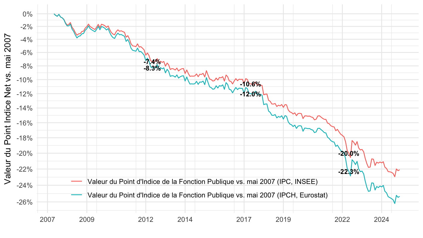
2007-
Code
net_brut_mensuel <- read_parquet(here::here("data", "insee", "INDICE-TRAITEMENT-FP-net-brut-mensuel.parquet"))
indicefp |>
  select(date, point_indice_en_euros) |>
  arrange(desc(date)) |>
  gather(variable, value, -date) |>
  group_by(variable) |>
  complete(date = seq.Date(min(date), max(date), by = "day")) |>
  fill(value) |>
  ungroup() |>
  left_join(cpi2_m, by = "date") |>
  filter(day(date) == 1) |>
  left_join(net_brut_mensuel, by = "date") |>
  filter(date >= as.Date("2007-01-01")) |>
  transmute(date,
            `Valeur du Point d'Indice de la Fonction Publique vs. 2007 (IPCH, Eurostat)` = (value/value[1])*(cpih[1]/cpih)*net_brut,
            `Valeur du Point d'Indice de la Fonction Publique vs. 2007 (IPC, INSEE)` = (value/value[1])*(cpi[1]/cpi)*net_brut) |>
  gather(variable, OBS_VALUE, -date) |>
  ggplot() + geom_line(aes(x = date, y = OBS_VALUE, color = variable)) + theme_minimal() +
  scale_x_date(breaks = c(seq(1999, 2100, 5), seq(1997, 2100, 5)) |> paste0("-01-01") |> as.Date(),
               labels = date_format("%Y")) +
  theme(legend.position = c(0.43, 0.12),
        legend.title = element_blank()) +
  scale_y_log10(breaks = seq(1, 0.02, -0.02),
                labels = percent(seq(1, 0.02, -0.02)-1, acc = 1)) +
  ylab("Valeur du Point Indice Fonction Publique vs. 2007") + xlab("") +
  geom_text_repel(data = . %>% filter(year(date) %in% seq(1999, 2040, 5),
                                month(date) == 1),
            aes(x = date, y = OBS_VALUE, label = percent(OBS_VALUE-1, acc = 0.1)),
                  fontface ="bold", color = "black", size = 3)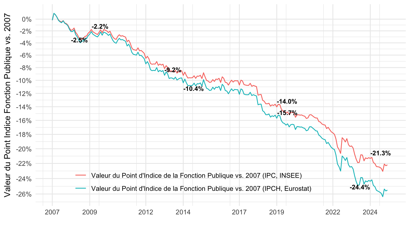
2017-
Code
net_brut_mensuel <- read_parquet(here::here("data", "insee", "INDICE-TRAITEMENT-FP-net-brut-mensuel.parquet"))
indicefp |>
  select(date, point_indice_en_euros) |>
  arrange(desc(date)) |>
  gather(variable, value, -date) |>
  group_by(variable) |>
  complete(date = seq.Date(min(date), max(date), by = "day")) |>
  fill(value) |>
  ungroup() |>
  left_join(cpi2_m, by = "date") |>
  filter(day(date) == 1) |>
  left_join(net_brut_mensuel, by = "date") |>
  filter(date >= as.Date("2017-01-01")) |>
  transmute(date,
            `Valeur du Point d'Indice de la Fonction Publique vs. 2017 (IPCH, Eurostat)` = (value/value[1])*(cpih[1]/cpih)*(net_brut/net_brut[1]),
            `Valeur du Point d'Indice de la Fonction Publique vs. 2017 (IPC, INSEE)` = (value/value[1])*(cpi[1]/cpi)*(net_brut/net_brut[1])) |>
  gather(variable, OBS_VALUE, -date) |>
  ggplot() + geom_line(aes(x = date, y = OBS_VALUE, color = variable)) + theme_minimal() +
  scale_x_date(breaks = c(seq(1999, 2100, 1), seq(1997, 2100, 5)) |> paste0("-01-01") |> as.Date(),
               labels = date_format("%Y")) +
  theme(legend.position = c(0.43, 0.12),
        legend.title = element_blank()) +
  scale_y_log10(breaks = seq(1, 0.02, -0.02),
                labels = percent(seq(1, 0.02, -0.02)-1, acc = 1)) +
  ylab("Valeur du Point Indice Net vs. 2017") + xlab("") +
  geom_text(data = . %>% filter(date %in% c(max(date), as.Date("2022-01-01"))),
            aes(x = date, y = OBS_VALUE, label = percent(OBS_VALUE-1, acc = 0.1)),
                  fontface ="bold", color = "black", size = 3)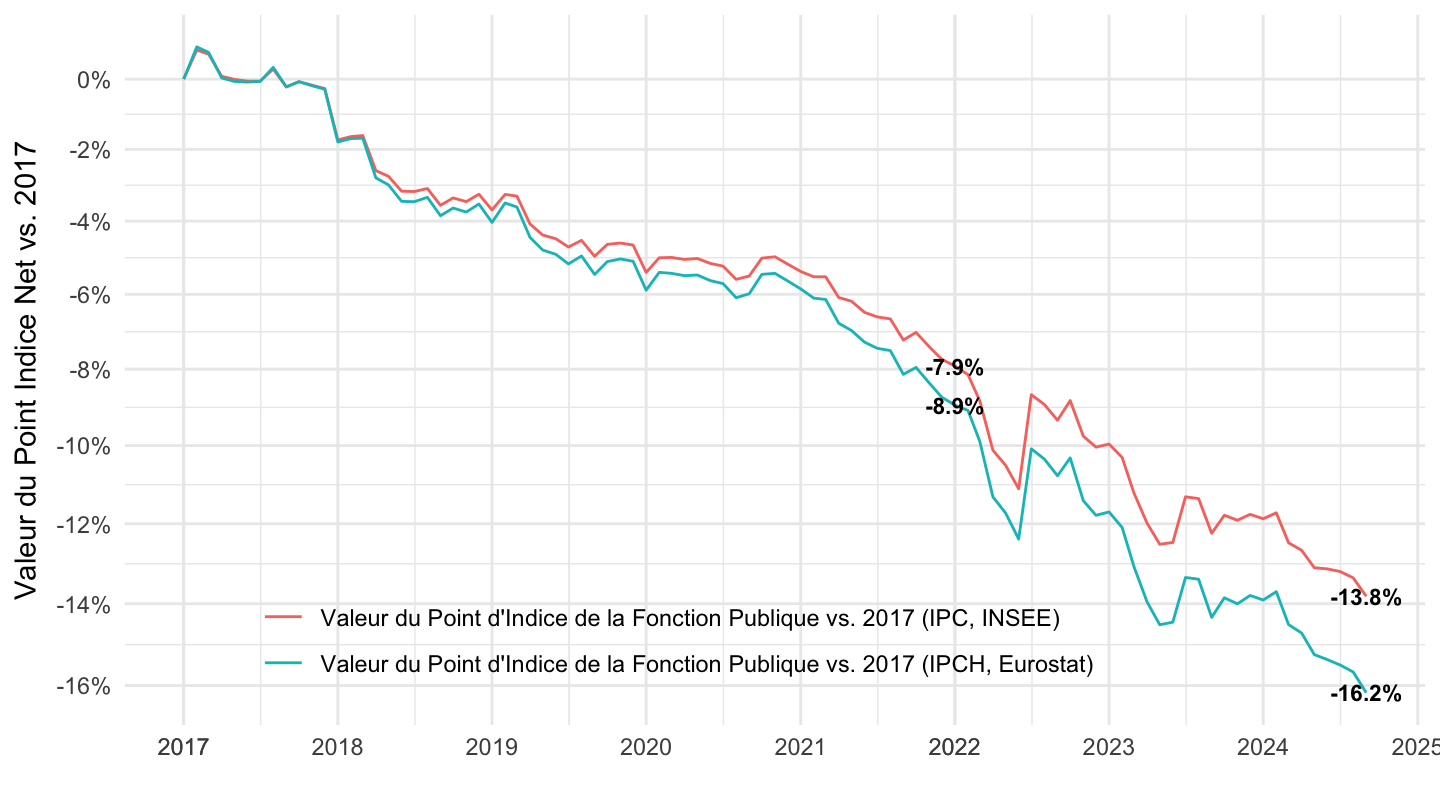
1997T1-
Code
net_brut_mensuel <- read_parquet(here::here("data", "insee", "INDICE-TRAITEMENT-FP-net-brut-mensuel.parquet"))

colors_fp <- c(
  "Pouvoir d'achat du Point d'Indice Net vs. 1996 (IPC, INSEE)"     = "#E07B6A",
  "Pouvoir d'achat du Point d'Indice Net vs. 1996 (IPCH, Eurostat)" = "#4ABFB0"
)

indicefp |>
  select(date, point_indice_en_euros) |>
  arrange(desc(date)) |>
  gather(variable, value, -date) |>
  group_by(variable) |>
  complete(date = seq.Date(min(date), max(date), by = "day")) |>
  fill(value) |>
  ungroup() |>
  left_join(cpi2_m, by = "date") |>
  filter(day(date) == 1) |>
  left_join(net_brut_mensuel, by = "date") |>
  filter(date >= as.Date("1996-02-01")) |>
  transmute(
    date,
    `Pouvoir d'achat du Point d'Indice Net vs. 1996 (IPCH, Eurostat)` = (value/value[1])*(cpih[1]/cpih)*(net_brut/net_brut[1]),
    `Pouvoir d'achat du Point d'Indice Net vs. 1996 (IPC, INSEE)`     = (value/value[1])*(cpi[1]/cpi)*(net_brut/net_brut[1])
  ) |>
  gather(variable, OBS_VALUE, -date) |>
  ggplot(aes(x = date, y = OBS_VALUE, color = variable)) +

  # Shaded area under each line
#geom_area(aes(fill = variable), alpha = 0.08, position = "identity") +
  geom_line(linewidth = 0.8) +

  # Horizontal reference line at 0%
  geom_hline(yintercept = 1, linetype = "dashed", color = "grey40", linewidth = 0.4) +

  # End labels
  geom_label(
    data        = . %>% group_by(variable) %>% filter(date == max(date)),
    aes(label   = percent(OBS_VALUE - 1, accuracy = 0.1)),
    fontface    = "bold",
    size        = 3.8,
    label.r     = unit(0.25, "lines"),
    label.padding = unit(0.3, "lines"),
    show.legend = FALSE
  ) +

  scale_color_manual(values = colors_fp) +
  scale_fill_manual(values  = colors_fp) +

  scale_x_date(
    breaks = c(seq(1996, 2100, 5)) |> paste0("-01-01") |> as.Date(),
    labels = date_format("%Y"),
    expand = expansion(mult = c(0.01, 0.06))   # breathing room on the right for labels
  ) +
  scale_y_continuous(
    breaks = seq(1, 0.50, -0.02),
    labels = percent(seq(1, 0.50, -0.02) - 1, accuracy = 1),
    expand = expansion(mult = c(0.02, 0.02))
  ) +

  labs(
    title    = "Pouvoir d'achat du point d'indice de la fonction publique vs. 1996",
    subtitle = "Valeur du point d'indice déflatée par l'IPC (préféré par l'Insee) et l'IPCH (préféré par Eurostat)",
    x = NULL, y = NULL,
    caption  = ""
  ) +

  theme_minimal(base_family = "sans") +
  theme(
    plot.title       = element_text(face = "bold", size = 13, margin = margin(b = 4)),
    plot.subtitle    = element_text(size = 10, color = "grey40", margin = margin(b = 10)),
    plot.caption     = element_text(size = 8,  color = "grey55", hjust = 0),
    legend.position  = c(0.4, 0.12),
    legend.title     = element_blank(),
    legend.text      = element_text(size = 9),
    legend.background = element_rect(fill = alpha("white", 0.7), color = NA),
    panel.grid.minor = element_blank(),
    panel.grid.major = element_line(color = "grey92"),
    axis.text        = element_text(size = 9, color = "grey40"),
    plot.margin      = margin(10, 15, 10, 10)
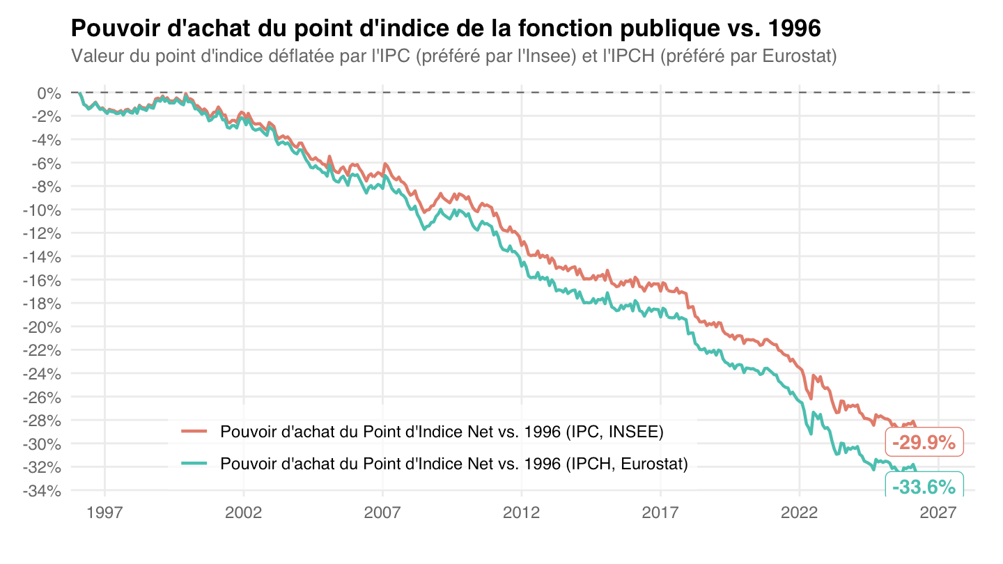
  )
2000-
Code
net_brut_mensuel <- read_parquet(here::here("data", "insee", "INDICE-TRAITEMENT-FP-net-brut-mensuel.parquet"))

colors_fp <- c(
  "Pouvoir d'achat du Point d'Indice Net vs. 2000 (IPC, INSEE)"     = "#E07B6A",
  "Pouvoir d'achat du Point d'Indice Net vs. 2000 (IPCH, Eurostat)" = "#4ABFB0"
)

indicefp |>
  select(date, point_indice_en_euros) |>
  arrange(desc(date)) |>
  gather(variable, value, -date) |>
  group_by(variable) |>
  complete(date = seq.Date(min(date), max(date), by = "day")) |>
  fill(value) |>
  ungroup() |>
  left_join(cpi2_m, by = "date") |>
  filter(day(date) == 1) |>
  left_join(net_brut_mensuel, by = "date") |>
  filter(date >= as.Date("2000-01-01")) |>
  transmute(
    date,
    `Pouvoir d'achat du Point d'Indice Net vs. 2000 (IPCH, Eurostat)` = (value/value[1])*(cpih[1]/cpih)*(net_brut/net_brut[1]),
    `Pouvoir d'achat du Point d'Indice Net vs. 2000 (IPC, INSEE)`     = (value/value[1])*(cpi[1]/cpi)*(net_brut/net_brut[1])
  ) |>
  gather(variable, OBS_VALUE, -date) |>
  ggplot(aes(x = date, y = OBS_VALUE, color = variable)) +

  # Shaded area under each line
#geom_area(aes(fill = variable), alpha = 0.08, position = "identity") +
  geom_line(linewidth = 0.8) +

  # Horizontal reference line at 0%
  geom_hline(yintercept = 1, linetype = "dashed", color = "grey40", linewidth = 0.4) +

  # End labels
  geom_label(
    data        = . %>% group_by(variable) %>% filter(date == max(date)),
    aes(label   = percent(OBS_VALUE - 1, accuracy = 0.1)),
    fontface    = "bold",
    size        = 3.8,
    label.r     = unit(0.25, "lines"),
    label.padding = unit(0.3, "lines"),
    show.legend = FALSE
  ) +

  scale_color_manual(values = colors_fp) +
  scale_fill_manual(values  = colors_fp) +

  scale_x_date(
    breaks = c(seq(2000, 2100, 2)) |> paste0("-01-01") |> as.Date(),
    labels = date_format("%Y"),
    expand = expansion(mult = c(0.01, 0.06))   # breathing room on the right for labels
  ) +
  scale_y_continuous(
    breaks = seq(1, 0.50, -0.02),
    labels = percent(seq(1, 0.50, -0.02) - 1, accuracy = 1),
    expand = expansion(mult = c(0.02, 0.02))
  ) +

  labs(
    title    = "Pouvoir d'achat du point d'indice de la fonction publique vs. 2000",
    subtitle = "Valeur du point d'indice déflatée par l'IPC (préféré par l'Insee) et l'IPCH (préféré par Eurostat)",
    x = NULL, y = NULL,
    caption  = ""
  ) +

  theme_minimal(base_family = "sans") +
  theme(
    plot.title       = element_text(face = "bold", size = 13, margin = margin(b = 4)),
    plot.subtitle    = element_text(size = 10, color = "grey40", margin = margin(b = 10)),
    plot.caption     = element_text(size = 8,  color = "grey55", hjust = 0),
    legend.position  = c(0.4, 0.12),
    legend.title     = element_blank(),
    legend.text      = element_text(size = 9),
    legend.background = element_rect(fill = alpha("white", 0.7), color = NA),
    panel.grid.minor = element_blank(),
    panel.grid.major = element_line(color = "grey92"),
    axis.text        = element_text(size = 9, color = "grey40"),
    plot.margin      = margin(10, 15, 10, 10)
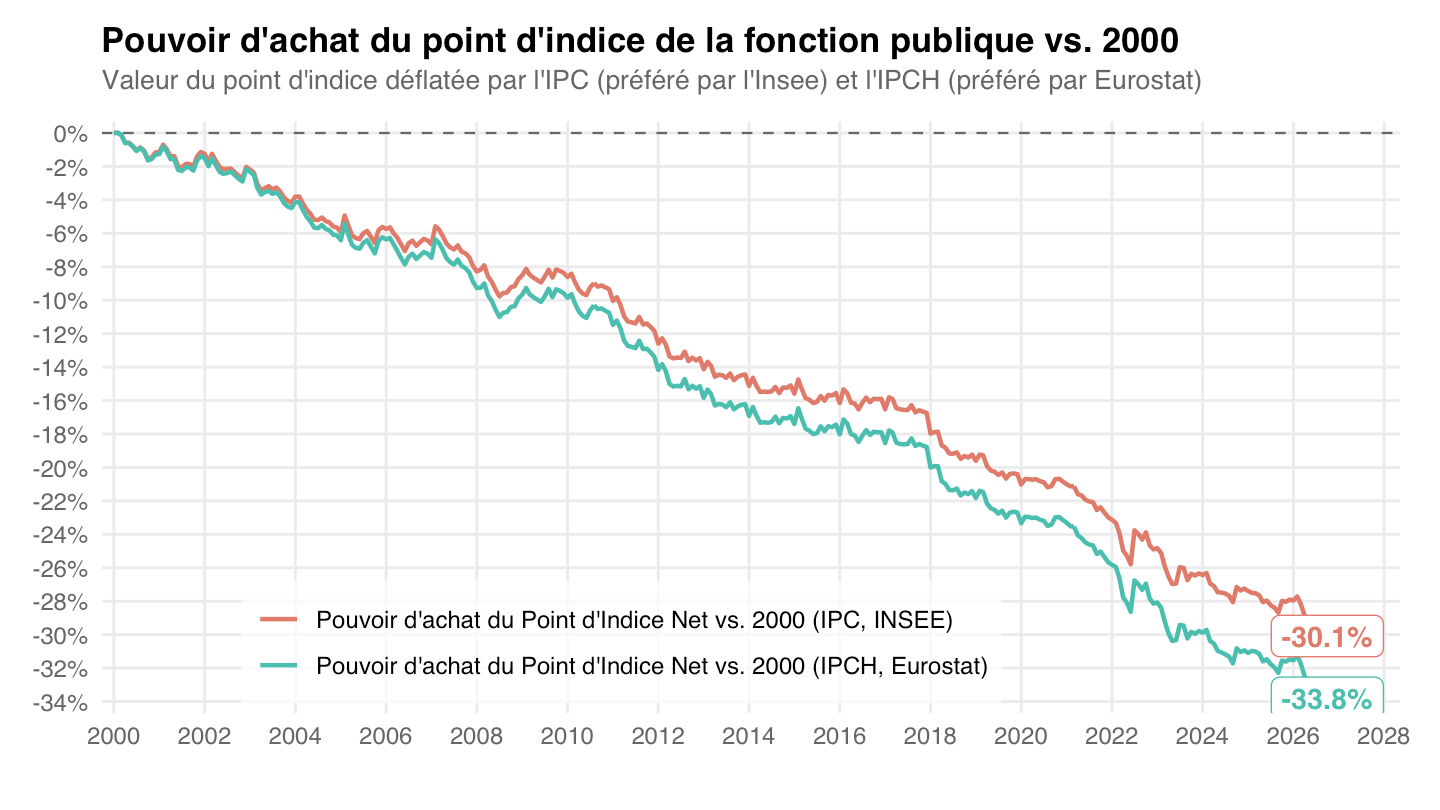
  )
2017T1-
Code
net_brut_mensuel <- read_parquet(here::here("data", "insee", "INDICE-TRAITEMENT-FP-net-brut-mensuel.parquet"))

colors_fp <- c(
  "Pouvoir d'achat du Point d'Indice Net vs. 2017 (IPC, INSEE)"     = "#E07B6A",
  "Pouvoir d'achat du Point d'Indice Net vs. 2017 (IPCH, Eurostat)" = "#4ABFB0"
)

indicefp |>
  select(date, point_indice_en_euros) |>
  arrange(desc(date)) |>
  gather(variable, value, -date) |>
  group_by(variable) |>
  complete(date = seq.Date(min(date), max(date), by = "day")) |>
  fill(value) |>
  ungroup() |>
  left_join(cpi2_m, by = "date") |>
  filter(day(date) == 1) |>
  left_join(net_brut_mensuel, by = "date") |>
  filter(date >= as.Date("2017-01-01")) |>
  transmute(
    date,
    `Pouvoir d'achat du Point d'Indice Net vs. 2017 (IPCH, Eurostat)` = (value/value[1])*(cpih[1]/cpih)*(net_brut/net_brut[1]),
    `Pouvoir d'achat du Point d'Indice Net vs. 2017 (IPC, INSEE)`     = (value/value[1])*(cpi[1]/cpi)*(net_brut/net_brut[1])
  ) |>
  gather(variable, OBS_VALUE, -date) |>
  ggplot(aes(x = date, y = OBS_VALUE, color = variable)) +

  # Shaded area under each line
#geom_area(aes(fill = variable), alpha = 0.08, position = "identity") +
  geom_line(linewidth = 0.8) +

  # Horizontal reference line at 0%
  geom_hline(yintercept = 1, linetype = "dashed", color = "grey40", linewidth = 0.4) +

  # End labels
  geom_label(
    data        = . %>% group_by(variable) %>% filter(date == max(date)),
    aes(label   = percent(OBS_VALUE - 1, accuracy = 0.1)),
    fontface    = "bold",
    size        = 3.8,
    label.r     = unit(0.25, "lines"),
    label.padding = unit(0.3, "lines"),
    show.legend = FALSE
  ) +

  scale_color_manual(values = colors_fp) +
  scale_fill_manual(values  = colors_fp) +

  scale_x_date(
    breaks = c(seq(1999, 2100, 1), seq(1997, 2100, 5)) |> paste0("-01-01") |> as.Date(),
    labels = date_format("%Y"),
    expand = expansion(mult = c(0.01, 0.06))   # breathing room on the right for labels
  ) +
  scale_y_continuous(
    breaks = seq(1, 0.80, -0.02),
    labels = percent(seq(1, 0.80, -0.02) - 1, accuracy = 1),
    expand = expansion(mult = c(0.02, 0.02))
  ) +

  labs(
    title    = "Pouvoir d'achat du point d'indice de la fonction publique vs. 2017",
    subtitle = "Valeur du point d'indice déflatée par l'IPC (préféré par l'Insee) et l'IPCH (préféré par Eurostat)",
    x = NULL, y = NULL,
    caption  = ""
  ) +

  theme_minimal(base_family = "sans") +
  theme(
    plot.title       = element_text(face = "bold", size = 13, margin = margin(b = 4)),
    plot.subtitle    = element_text(size = 10, color = "grey40", margin = margin(b = 10)),
    plot.caption     = element_text(size = 8,  color = "grey55", hjust = 0),
    legend.position  = c(0.33, 0.12),
    legend.title     = element_blank(),
    legend.text      = element_text(size = 9),
    legend.background = element_rect(fill = alpha("white", 0.7), color = NA),
    panel.grid.minor = element_blank(),
    panel.grid.major = element_line(color = "grey92"),
    axis.text        = element_text(size = 9, color = "grey40"),
    plot.margin      = margin(10, 15, 10, 10)
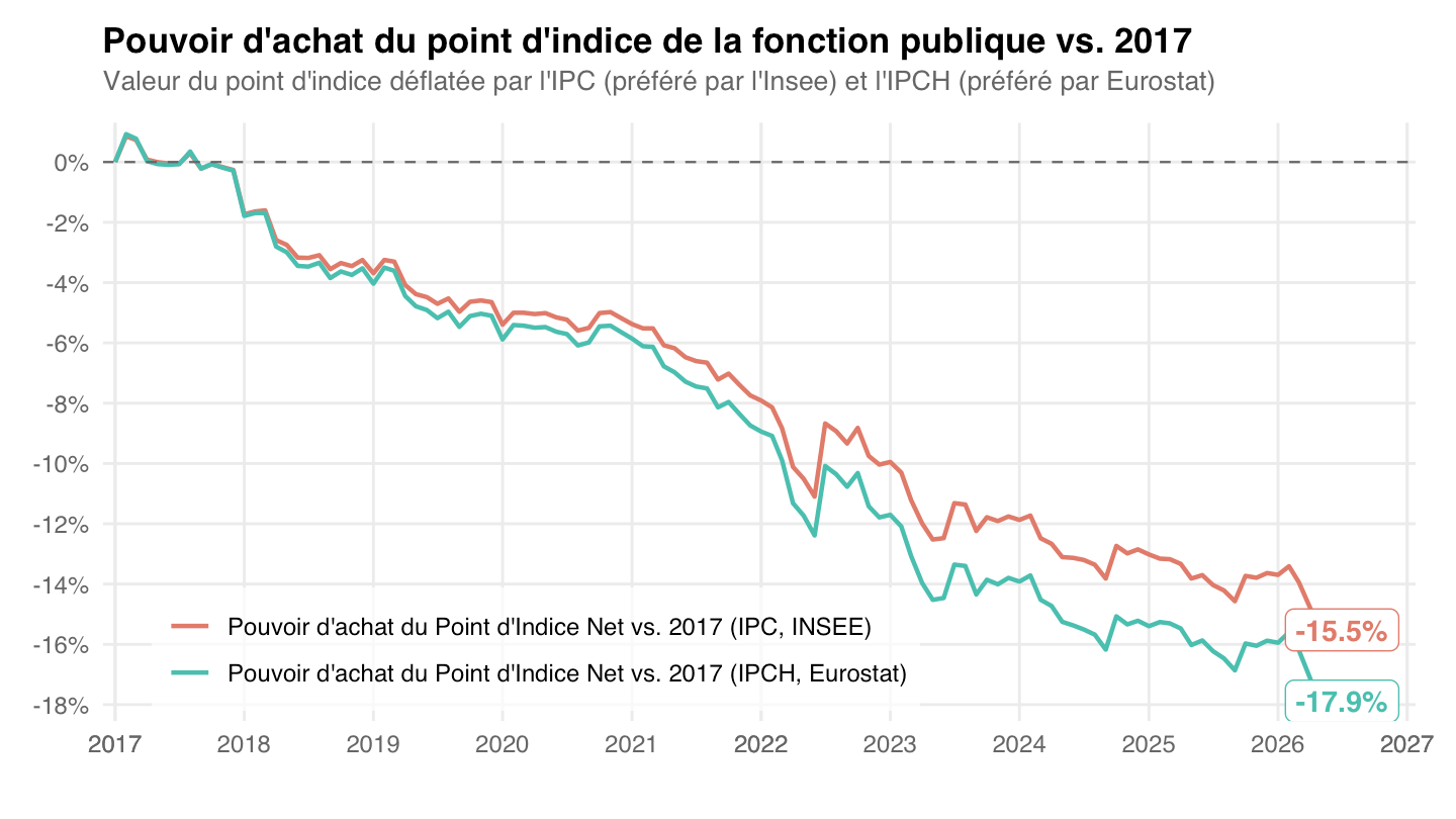
  )
2017T2-
Code
net_brut_mensuel <- read_parquet(here::here("data", "insee", "INDICE-TRAITEMENT-FP-net-brut-mensuel.parquet"))

colors_fp <- c(
  "Pouvoir d'achat du Point d'Indice Net vs. 2017 (IPC, INSEE)"     = "#E07B6A",
  "Pouvoir d'achat du Point d'Indice Net vs. 2017 (IPCH, Eurostat)" = "#4ABFB0"
)

indicefp |>
  select(date, point_indice_en_euros) |>
  arrange(desc(date)) |>
  gather(variable, value, -date) |>
  group_by(variable) |>
  complete(date = seq.Date(min(date), max(date), by = "day")) |>
  fill(value) |>
  ungroup() |>
  left_join(cpi2_m, by = "date") |>
  filter(day(date) == 1) |>
  left_join(net_brut_mensuel, by = "date") |>
  filter(date >= as.Date("2017-06-01")) |>
  transmute(
    date,
    `Pouvoir d'achat du Point d'Indice Net vs. 2017 (IPCH, Eurostat)` = (value/value[1])*(cpih[1]/cpih)*(net_brut/net_brut[1]),
    `Pouvoir d'achat du Point d'Indice Net vs. 2017 (IPC, INSEE)`     = (value/value[1])*(cpi[1]/cpi)*(net_brut/net_brut[1])
  ) |>
  gather(variable, OBS_VALUE, -date) |>
  ggplot(aes(x = date, y = OBS_VALUE, color = variable)) +

  # Shaded area under each line
#geom_area(aes(fill = variable), alpha = 0.08, position = "identity") +
  geom_line(linewidth = 0.8) +

  # Horizontal reference line at 0%
  geom_hline(yintercept = 1, linetype = "dashed", color = "grey40", linewidth = 0.4) +

  # End labels
  geom_label(
    data        = . %>% group_by(variable) %>% filter(date == max(date)),
    aes(label   = percent(OBS_VALUE - 1, accuracy = 0.1)),
    fontface    = "bold",
    size        = 3.8,
    label.r     = unit(0.25, "lines"),
    label.padding = unit(0.3, "lines"),
    show.legend = FALSE
  ) +

  scale_color_manual(values = colors_fp) +
  scale_fill_manual(values  = colors_fp) +

  scale_x_date(
    breaks = c(seq(1999, 2100, 1), seq(1997, 2100, 5)) |> paste0("-01-01") |> as.Date(),
    labels = date_format("%Y"),
    expand = expansion(mult = c(0.01, 0.06))   # breathing room on the right for labels
  ) +
  scale_y_continuous(
    breaks = seq(1, 0.80, -0.02),
    labels = percent(seq(1, 0.80, -0.02) - 1, accuracy = 1),
    expand = expansion(mult = c(0.02, 0.02))
  ) +

  labs(
    title    = "Pouvoir d'achat du point d'indice de la fonction publique par rapport à 2017",
    subtitle = "Valeur du point d'indice déflatée par l'IPC (préféré par l'Insee) et l'IPCH (préféré par Eurostat)",
    x = NULL, y = NULL,
    caption  = ""
  ) +

  theme_minimal(base_family = "sans") +
  theme(
    plot.title       = element_text(face = "bold", size = 13, margin = margin(b = 4)),
    plot.subtitle    = element_text(size = 10, color = "grey40", margin = margin(b = 10)),
    plot.caption     = element_text(size = 8,  color = "grey55", hjust = 0),
    legend.position  = c(0.3, 0.12),
    legend.title     = element_blank(),
    legend.text      = element_text(size = 9),
    legend.background = element_rect(fill = alpha("white", 0.7), color = NA),
    panel.grid.minor = element_blank(),
    panel.grid.major = element_line(color = "grey92"),
    axis.text        = element_text(size = 9, color = "grey40"),
    plot.margin      = margin(10, 15, 10, 10)
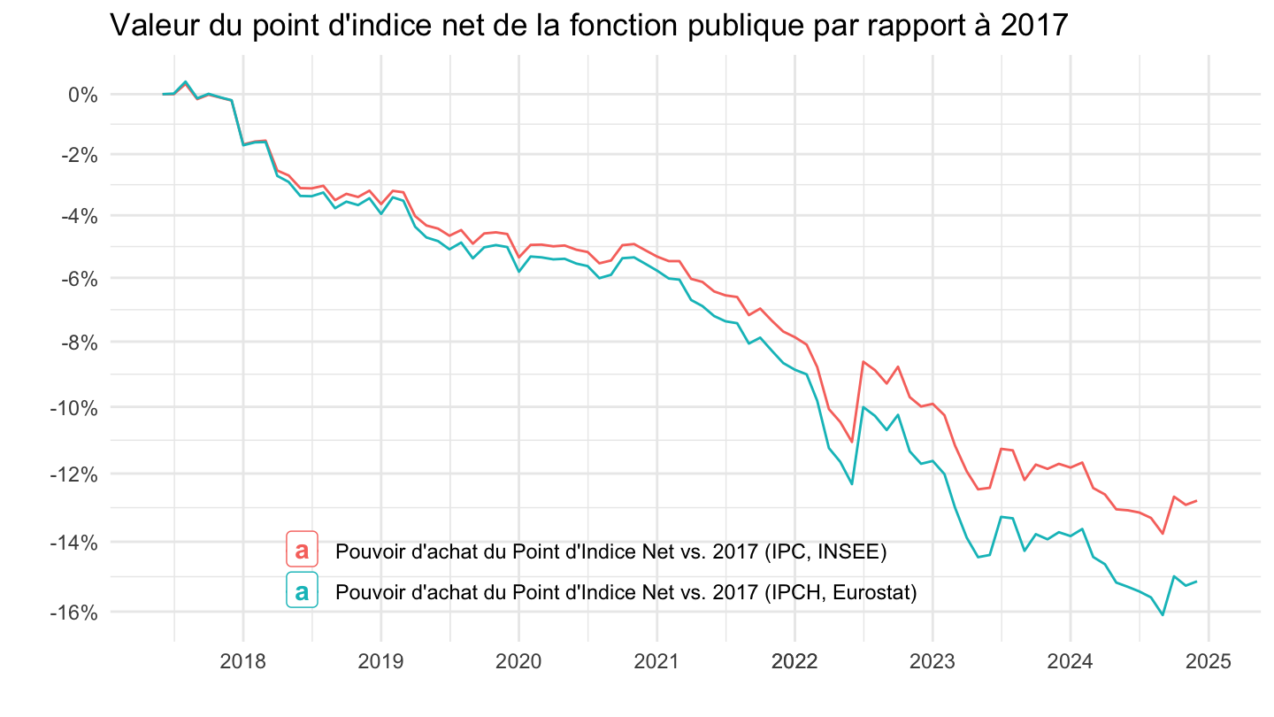
  )
2010-2018
Annuel
Code
indicefp |>
  select(date, point_indice_en_euros) |>

  arrange(desc(date)) |>
  gather(variable, value, -date) |>
  group_by(variable) |>
  complete(date = seq.Date(min(date), max(date), by = "day")) |>
  fill(value) |>
  filter(month(date) == 1,
         day(date) == 1) |>
  left_join(cpi, by = "date") |>
  filter(date >= as.Date("2010-01-01"),
         date <= as.Date("2018-01-01")) |>
  mutate(value = value/cpi,
         value = 100*value/value[1]) |>
  ggplot() + geom_line(aes(x = date, y = value)) + theme_minimal() +
  scale_x_date(breaks = seq(1920, 2100, 1) |> paste0("-01-01") |> as.Date(),
               labels = date_format("%Y")) +
  scale_y_log10(breaks = seq(0, 200, 1)) +
  ylab("Point Indice Fonction Publique (euros constants)") + xlab("")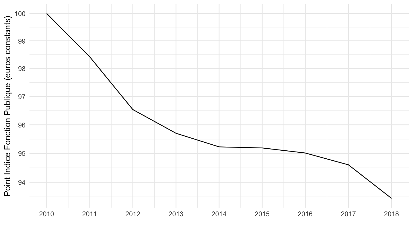
Related Data
Inflation in France: CPI or HICP ?
| source | dataset | Title | Updated |
|---|---|---|---|

Inflation en France: IPC ou IPCH ?
| source | dataset | Title | Updated |
|---|---|---|---|
Évolution du pouvoir d’achat
| source | dataset | Title | Updated |
|---|---|---|---|


Évolution du pouvoir d’achat depuis 2017
| source | dataset | Title | Updated |
|---|---|---|---|
