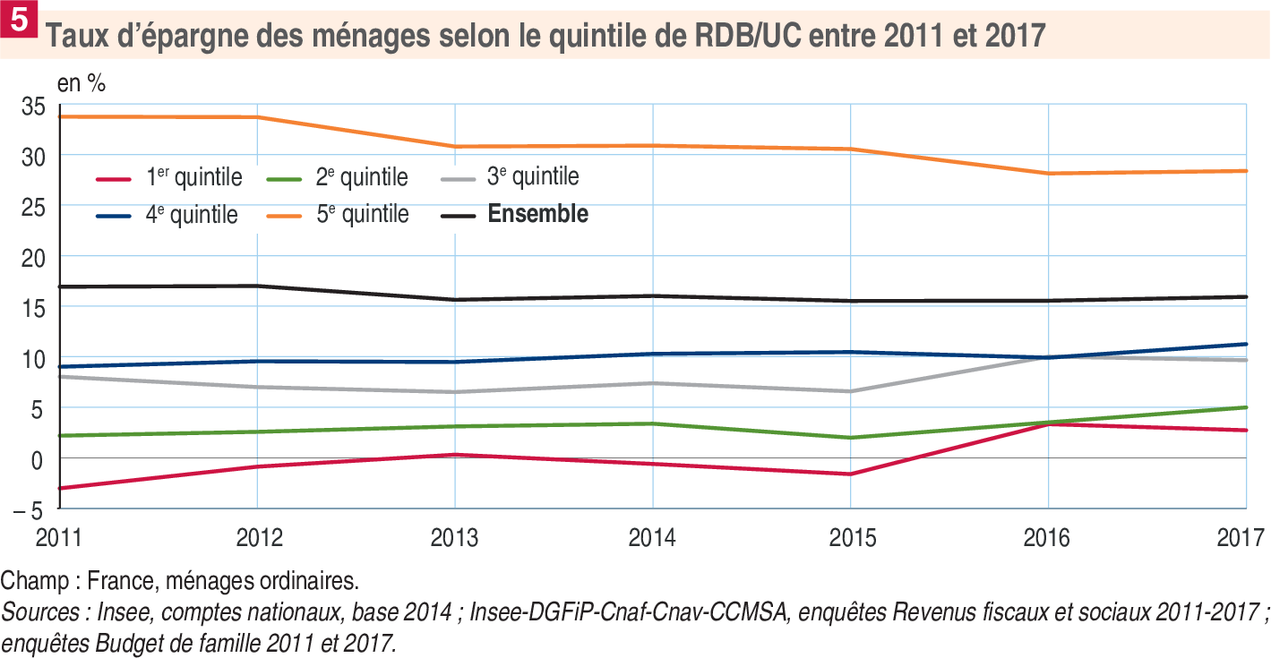
Plus d’épargne chez les plus aisés, plus de dépenses contraintes chez les plus modestes - ip1815
Données - INSEE
Info
Lien
Par catégorie
Age
Table
Code
ip1815 %>%
  filter(sheet == "fig6",
         grepl(" ans", type)) %>%
  mutate(`taux d'épargne` = round(100*(1-`Consommation / UC` / `Revenu Disponible Brut / UC`), 1)) %>%
  select(-sheet) %>%
print_table_conditional| type | Consommation / UC | Revenu Disponible Brut / UC | taux d'épargne |
|---|---|---|---|
| Moins de 30 ans | 17924 | 19562 | 8.4 |
| 30-39 ans | 23865 | 26210 | 8.9 |
| 40-49 ans | 25270 | 28509 | 11.4 |
| 50-59 ans | 27276 | 33169 | 17.8 |
| 60-69 ans | 27215 | 33150 | 17.9 |
| 70 ans ou plus | 25689 | 34346 | 25.2 |
Graph
Code
ip1815 %>%
  filter(sheet == "fig6",
         grepl(" ans", type)) %>%
  ggplot(., aes(x = `Revenu Disponible Brut / UC`, y = `Consommation / UC`)) + geom_point() +
  theme_minimal() + geom_abline(slope = 1) +
  scale_x_continuous(breaks = seq(0, 100000, 2000),
                     labels = dollar_format(pre = "", su = " €")) +
  scale_y_continuous(breaks = seq(0, 100000, 2000),
                     labels = dollar_format(pre = "", su = " €")) +
  geom_text_repel(aes(x = `Revenu Disponible Brut / UC`, y = `Consommation / UC`, label = type),
                  fontface ="plain", color = "black", size = 3)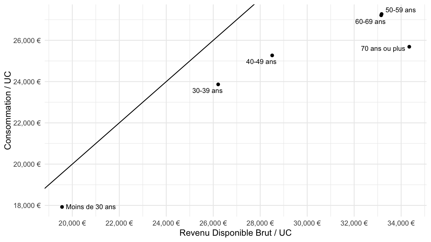
Taux d’épargne
Code
ip1815 %>%
  filter(sheet == "fig6",
         grepl(" ans", type)) %>%
  ggplot(., aes(x = `Revenu Disponible Brut / UC`, y = 1-`Consommation / UC` / `Revenu Disponible Brut / UC`)) + geom_point(size = 3) +
  theme_minimal() + geom_abline(slope = 1) + ylab("Taux d'épargne (%)") +
  xlab("Revenu Disponible Brut par Unité de Consommation") +
  theme(axis.text.x = element_text(angle = 45, vjust = 1, hjust = 1)) +
  scale_x_continuous(breaks = seq(0, 100000, 1000),
                     labels = dollar_format(pre = "", su = " €")) +
  scale_y_continuous(breaks = 0.01*seq(0, 100, 1),
                     labels = percent_format(acc = 1)) +
  geom_text_repel(aes(x = `Revenu Disponible Brut / UC`, y = 1-`Consommation / UC` / `Revenu Disponible Brut / UC`-0.005, label = type),
                  fontface ="plain", color = "red", size = 5)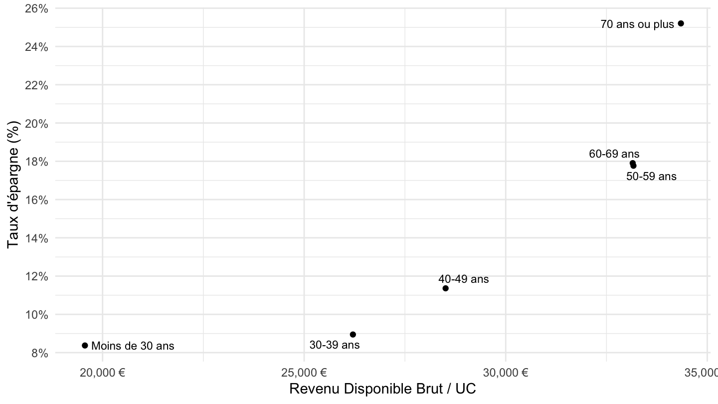
Quintile
Table
Code
ip1815 %>%
  filter(sheet == "fig6",
         grepl("quintile", type)) %>%
  mutate(`taux d'épargne` = round(100*(1-`Consommation / UC` / `Revenu Disponible Brut / UC`), 1)) %>%
  select(-sheet) %>%
print_table_conditional| type | Consommation / UC | Revenu Disponible Brut / UC | taux d'épargne |
|---|---|---|---|
| 1er quintile | 12816 | 13173 | 2.7 |
| 2e quintile | 19262 | 20273 | 5.0 |
| 3e quintile | 23592 | 26112 | 9.7 |
| 4e quintile | 29029 | 32702 | 11.2 |
| 5e quintile | 40222 | 56153 | 28.4 |
Fonction de consommation
Fit
Linéaire:
Code
fit_lineaire <- ip1815 %>%
  filter(sheet == "fig6",
         grepl("quintile", type)) %>%
  lm(`Consommation / UC` ~ `Revenu Disponible Brut / UC`, data = .) %>%
  summary()

fit_lineaire
#
# Call:
# lm(formula = `Consommation / UC` ~ `Revenu Disponible Brut / UC`,
# data = .)
#
# Residuals:
# 1 2 3 4 5
# -1880.4 141.3 832.8 2163.3 -1257.0
#
# Coefficients:
# Estimate Std. Error t value Pr(>|t|)
# (Intercept) 6.488e+03 1.884e+03 3.444 0.04112 *
# `Revenu Disponible Brut / UC` 6.231e-01 5.686e-02 10.960 0.00163 **
# ---
# Signif. codes: 0 '***' 0.001 '**' 0.01 '*' 0.05 '.' 0.1 ' ' 1
#
# Residual standard error: 1872 on 3 degrees of freedom
# Multiple R-squared: 0.9756, Adjusted R-squared: 0.9675
# F-statistic: 120.1 on 1 and 3 DF, p-value: 0.001626Log:
Code
fit_log <- ip1815 %>%
  filter(sheet == "fig6",
         grepl("quintile", type)) %>%
  lm(log(`Consommation / UC`) ~ log(`Revenu Disponible Brut / UC`), data = .) %>%
  summary()

fit_log
#
# Call:
# lm(formula = log(`Consommation / UC`) ~ log(`Revenu Disponible Brut / UC`),
# data = .)
#
# Residuals:
# 1 2 3 4 5
# -0.04586 0.02040 0.02287 0.05216 -0.04957
#
# Coefficients:
# Estimate Std. Error t value Pr(>|t|)
# (Intercept) 1.99735 0.49356 4.047 0.027167 *
# log(`Revenu Disponible Brut / UC`) 0.79138 0.04842 16.342 0.000499 ***
# ---
# Signif. codes: 0 '***' 0.001 '**' 0.01 '*' 0.05 '.' 0.1 ' ' 1
#
# Residual standard error: 0.05235 on 3 degrees of freedom
# Multiple R-squared: 0.9889, Adjusted R-squared: 0.9852
# F-statistic: 267.1 on 1 and 3 DF, p-value: 0.0004985Log10:
Code
ip1815 %>%
  filter(sheet == "fig6",
         grepl("quintile", type)) %>%
  lm(log10(`Consommation / UC`) ~ log10(`Revenu Disponible Brut / UC`), data = .) %>%
  summary()
#
# Call:
# lm(formula = log10(`Consommation / UC`) ~ log10(`Revenu Disponible Brut / UC`),
# data = .)
#
# Residuals:
# 1 2 3 4 5
# -0.019917 0.008859 0.009932 0.022655 -0.021528
#
# Coefficients:
# Estimate Std. Error t value Pr(>|t|)
# (Intercept) 0.86744 0.21435 4.047 0.027167 *
# log10(`Revenu Disponible Brut / UC`) 0.79138 0.04842 16.342 0.000499 ***
# ---
# Signif. codes: 0 '***' 0.001 '**' 0.01 '*' 0.05 '.' 0.1 ' ' 1
#
# Residual standard error: 0.02273 on 3 degrees of freedom
# Multiple R-squared: 0.9889, Adjusted R-squared: 0.9852
# F-statistic: 267.1 on 1 and 3 DF, p-value: 0.0004985Elasticité:
Code
log(40222/12816)/log(56153/13173)# [1] 0.7888207Linéaire
Code
ip1815 %>%
  filter(sheet == "fig6",
         grepl("quintile", type)) %>%
  ggplot(., aes(x = `Revenu Disponible Brut / UC`, y = `Consommation / UC`)) + geom_point() +
  theme_minimal() + geom_abline(slope = 1) +
  scale_x_continuous(breaks = seq(0, 100000, 5000),
                     labels = dollar_format(pre = "", su = " €")) +
  scale_y_continuous(breaks = seq(0, 100000, 5000),
                     labels = dollar_format(pre = "", su = " €")) +
  geom_text_repel(aes(x = `Revenu Disponible Brut / UC`, y = `Consommation / UC`, label = type),
                  fontface ="plain", color = "black", size = 3) +
  geom_function(fun = function(x) exp(fit_log$coefficients[1, 1] + fit_log$coefficients[2, 1]*log(x)), colour = "red")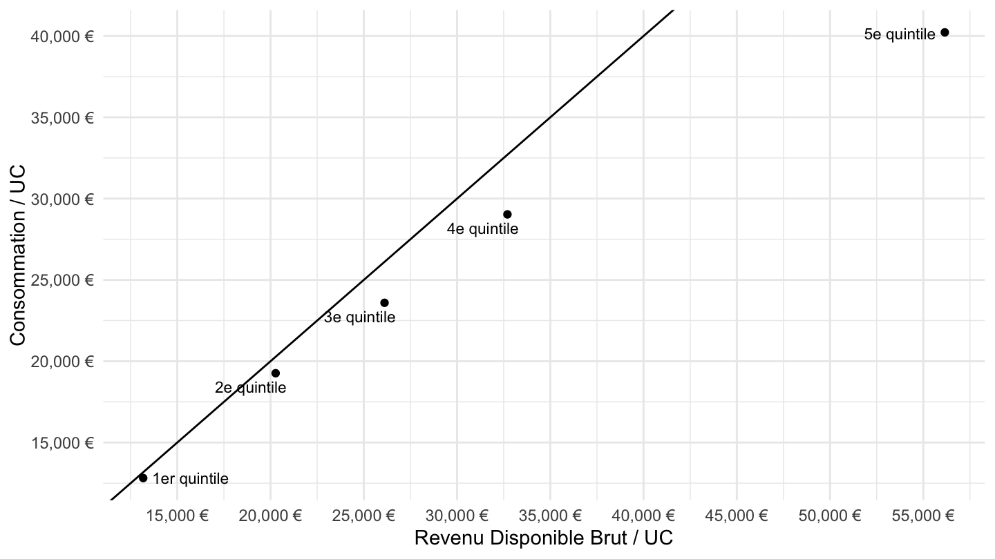
Log
Code
ip1815 %>%
  filter(sheet == "fig6",
         grepl("quintile", type)) %>%
  ggplot(., aes(x = `Revenu Disponible Brut / UC`, y = `Consommation / UC`)) + geom_point() +
  theme_minimal() +
  scale_x_log10(breaks = seq(0, 100000, 5000),
                     labels = dollar_format(pre = "", su = " €", acc = 1)) +
  scale_y_log10(breaks = seq(0, 100000, 5000),
                     labels = dollar_format(pre = "", su = " €", acc = 1)) +
  geom_text_repel(aes(x = `Revenu Disponible Brut / UC`, y = `Consommation / UC`, label = type),
                  fontface ="plain", color = "black", size = 3) +
  theme(axis.text.x = element_text(angle = 45, vjust = 1, hjust = 1),
        axis.text.y = element_text(angle = 45, vjust = 1, hjust = 1)) +
  geom_function(fun = function(x) exp(fit_log$coefficients[1, 1] + fit_log$coefficients[2, 1]*log(x)), colour = "red")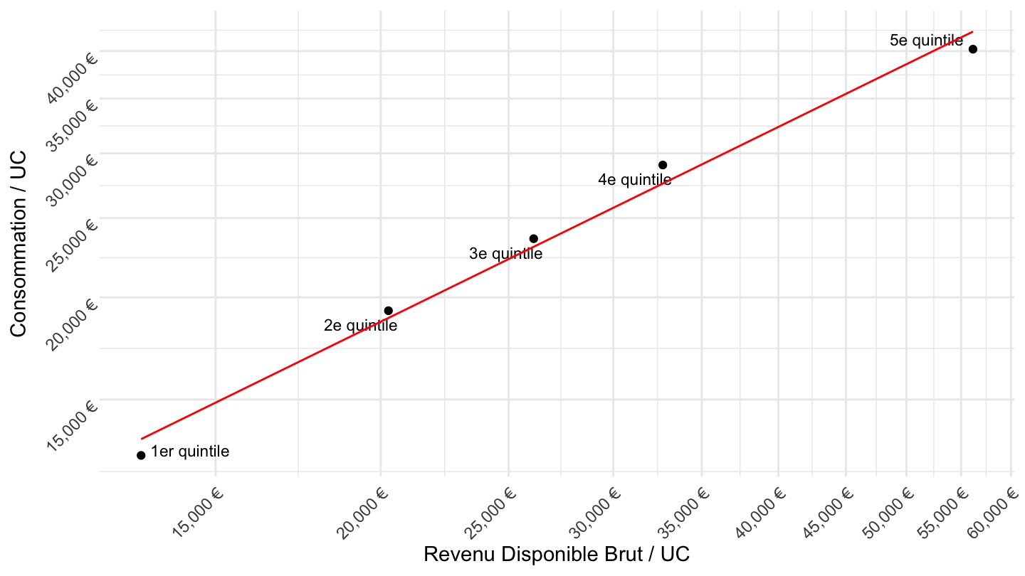
Extrapolation
\[7.3694838 \cdot C^{0.7913792}\]
Fit: 7.3694838 C puissance 0.7913792
Propension à épargner vs. taux d’épargne moyen
Code
fonction_consommation <- function(x) exp(fit_log$coefficients[1, 1] + fit_log$coefficients[2, 1]*log(x))

taux_epargne <- function(x) 1- fonction_consommation(x)/x
propension_epargner <- function(x) 1- fit_log$coefficients[2, 1]*fonction_consommation(x)/x

tibble(Revenu = seq(10000, 60000, 5000)) %>%
  mutate(`Taux d'épargne` = taux_epargne(Revenu),
         `Propension à épargner` = propension_epargner(Revenu)) %>%
  gather(variable, value, -Revenu) %>%
  ggplot(., aes(x = Revenu, y = value, color = variable)) + geom_point() +
  theme_minimal() + geom_abline(slope = 1) + ylab("Taux d'épargne (%)") +
  scale_x_continuous(breaks = seq(0, 100000, 5000),
                     labels = dollar_format(pre = "", su = " €")) +
  theme(axis.text.x = element_text(angle = 45, vjust = 1, hjust = 1)) +
  scale_y_continuous(breaks = 0.01*seq(-100, 100, 2),
                     labels = percent_format(acc = 1))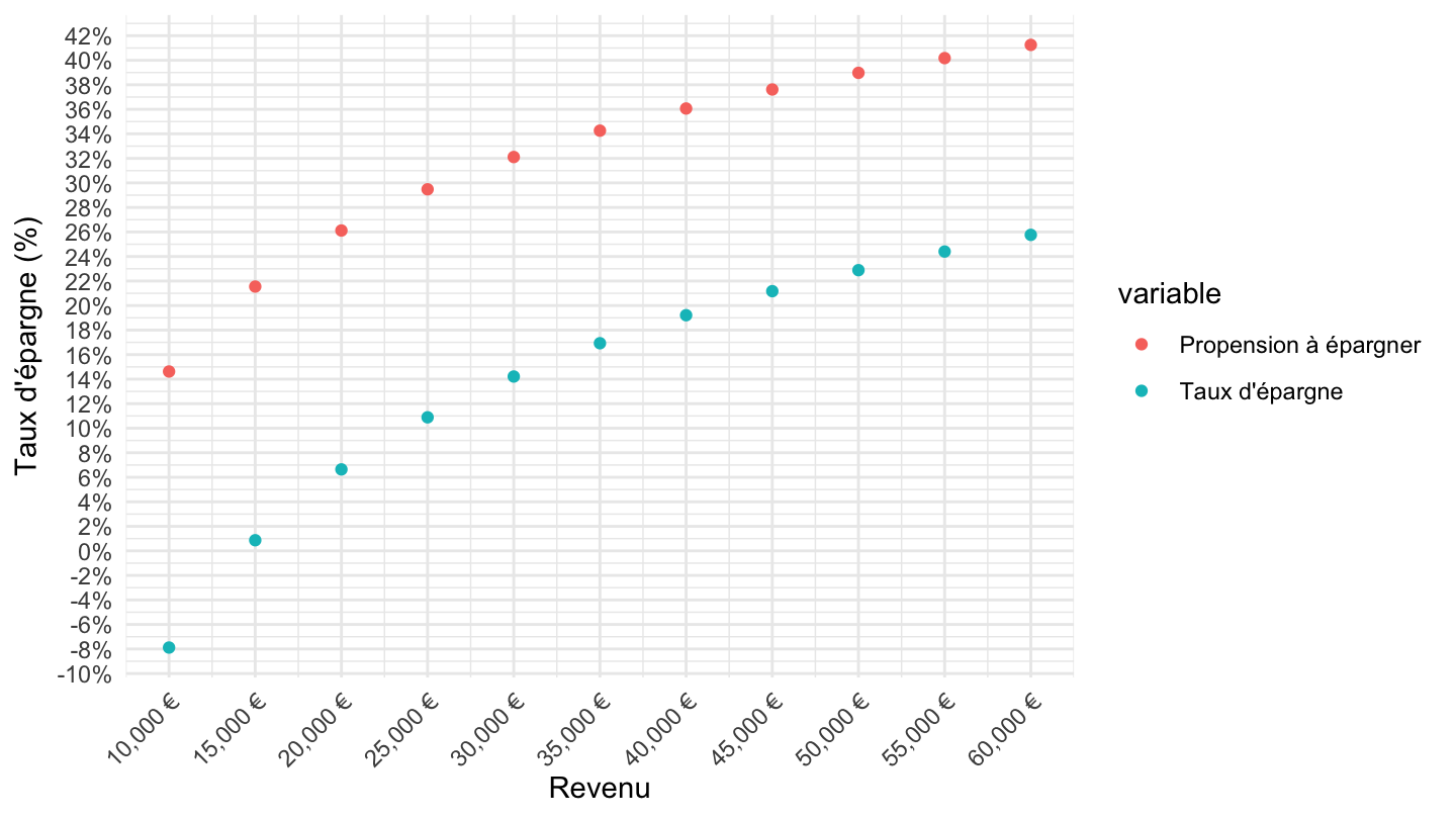
Code
fonction_consommation <- function(x) exp(fit_log$coefficients[1, 1] + fit_log$coefficients[2, 1]*log(x))

taux_epargne <- function(x) 1- fonction_consommation(x)/x
propension_epargner <- function(x) 1- fit_log$coefficients[2, 1]*fonction_consommation(x)/x

tibble(Revenu = seq(10000, 60000, 5000)) %>%
  mutate(`Taux d'épargne` = taux_epargne(Revenu),
         `Propension à épargner` = propension_epargner(Revenu)) %>%
  gather(variable, value, -Revenu) %>%
  ggplot(., aes(x = Revenu, y = value, color = variable)) + geom_point() +
  theme_minimal() + geom_abline(slope = 1) + ylab("Taux d'épargne (%)") +
  scale_x_log10(breaks = seq(0, 100000, 5000),
                     labels = dollar_format(pre = "", su = " €", acc = 1)) +
  theme(axis.text.x = element_text(angle = 45, vjust = 1, hjust = 1)) +
  scale_y_continuous(breaks = 0.01*seq(-100, 100, 2),
                     labels = percent_format(acc = 1))
Code
fonction_consommation <- function(x) exp(fit_log$coefficients[1, 1] + fit_log$coefficients[2, 1]*log(x))

taux_epargne <- function(x) 1- fonction_consommation(x)/x
propension_epargner <- function(x) 1- fit_log$coefficients[2, 1]*fonction_consommation(x)/x

tibble(Revenu = seq(10000, 1000000, 10000)) %>%
  mutate(`Taux d'épargne` = taux_epargne(Revenu),
         `Propension à épargner` = propension_epargner(Revenu)) %>%
  gather(variable, value, -Revenu) %>%
  ggplot(., aes(x = Revenu, y = value, color = variable)) + geom_point() +
  theme_minimal() + geom_abline(slope = 1) + ylab("Taux d'épargne (%)") +
  scale_x_log10(breaks = c(10000, 20000, 50000, 100000, 200000, 500000, 1000000),
                     labels = dollar_format(pre = "", su = " €", acc = 1)) +
  theme(axis.text.x = element_text(angle = 45, vjust = 1, hjust = 1)) +
  scale_y_continuous(breaks = 0.01*seq(-100, 100, 5),
                     labels = percent_format(acc = 1))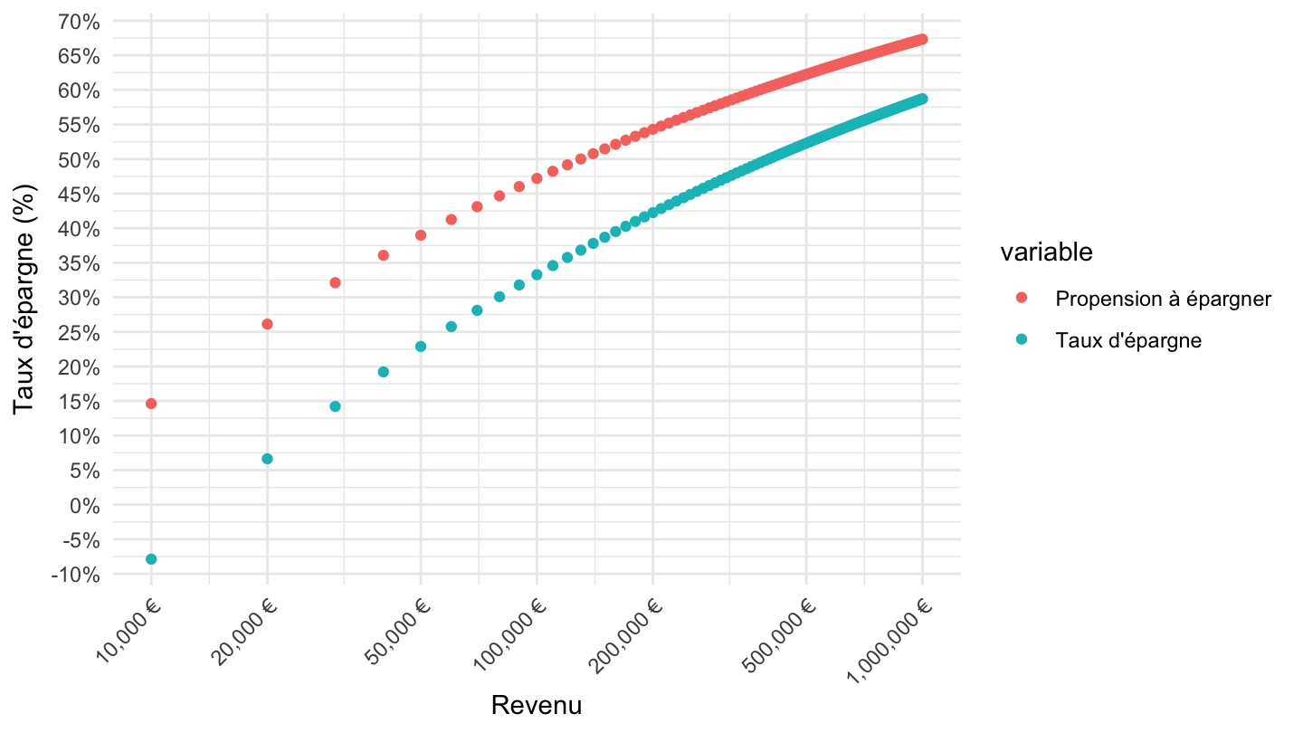
Taux d’épargne
Code
ip1815 %>%
  filter(sheet == "fig6",
         grepl("quintile", type)) %>%
  ggplot(., aes(x = `Revenu Disponible Brut / UC`, y = 1-`Consommation / UC` / `Revenu Disponible Brut / UC`)) + geom_point() +
  theme_minimal() + geom_abline(slope = 1) + ylab("Taux d'épargne (%)") +
  scale_x_continuous(breaks = seq(0, 100000, 5000),
                     labels = dollar_format(pre = "", su = " €")) +
  scale_y_continuous(breaks = 0.01*seq(0, 100, 2),
                     labels = percent_format(acc = 1)) +
  geom_text_repel(aes(x = `Revenu Disponible Brut / UC`, y = 1-`Consommation / UC` / `Revenu Disponible Brut / UC`, label = type),
                  fontface ="plain", color = "black", size = 3)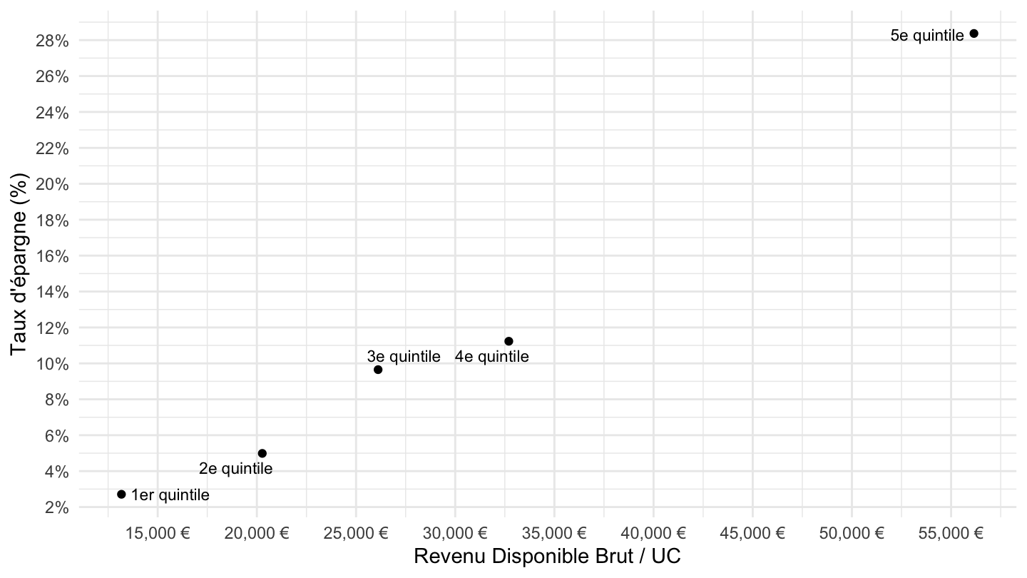
Categories sociales
Table
Code
ip1815 %>%
  filter(sheet == "fig6",
         !grepl("quintile", type),
         !grepl(" ans", type)) %>%
  mutate(`taux d'épargne` = round(100*(1-`Consommation / UC` / `Revenu Disponible Brut / UC`), 1)) %>%
  select(-sheet) %>%
print_table_conditional| type | Consommation / UC | Revenu Disponible Brut / UC | taux d'épargne |
|---|---|---|---|
| Agriculteurs | 21698 | 28937 | 25.0 |
| Indépendants et professions libérales | 25307 | 38739 | 34.7 |
| Cadres | 35946 | 42659 | 15.7 |
| Professions intermédiaires | 27910 | 32360 | 13.8 |
| Employés | 22178 | 18895 | -17.4 |
| Ouvriers | 20064 | 22894 | 12.4 |
| Retraités Agriculteurs | 19783 | 30303 | 34.7 |
| Retraités indépendants | 24533 | 35366 | 30.6 |
| Retraités cadres | 37112 | 44940 | 17.4 |
| Retraités professions intermédiaires | 28222 | 31441 | 10.2 |
| Retraités employés | 20931 | 23485 | 10.9 |
| Retraités ouvriers | 18495 | 21622 | 14.5 |
| Autres inactifs | 15417 | 22113 | 30.3 |
| Ensemble | 25184 | 29954 | 15.9 |
Fonction de consommation
Code
ip1815 %>%
  filter(sheet == "fig6",
         !grepl("quintile", type),
         !grepl(" ans", type)) %>%
  ggplot(., aes(x = `Revenu Disponible Brut / UC`, y = `Consommation / UC`)) + geom_point() +
  theme_minimal() + geom_abline(slope = 1) +
  scale_x_continuous(breaks = seq(0, 100000, 5000),
                     labels = dollar_format(pre = "", su = " €")) +
  scale_y_continuous(breaks = seq(0, 100000, 5000),
                     labels = dollar_format(pre = "", su = " €")) +
  geom_text_repel(aes(x = `Revenu Disponible Brut / UC`, y = `Consommation / UC`, label = type),
                  fontface ="plain", color = "black", size = 3)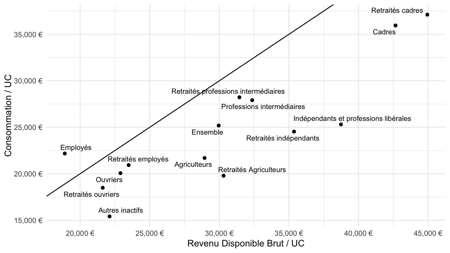
Taux d’épargne
Code
ip1815 %>%
  filter(sheet == "fig6",
         !grepl("quintile", type),
         !grepl(" ans", type)) %>%
  ggplot(., aes(x = `Revenu Disponible Brut / UC`, y = 1-`Consommation / UC` / `Revenu Disponible Brut / UC`)) + geom_point() +
  theme_minimal() + geom_abline(slope = 1) + ylab("Taux d'épargne (%)") +
  scale_x_continuous(breaks = seq(0, 100000, 5000),
                     labels = dollar_format(pre = "", su = " €")) +
  scale_y_continuous(breaks = 0.01*seq(-100, 100, 5),
                     labels = percent_format(acc = 1)) +
  geom_text_repel(aes(x = `Revenu Disponible Brut / UC`, y = 1-`Consommation / UC` / `Revenu Disponible Brut / UC`, label = type),
                  fontface ="plain", color = "black", size = 3)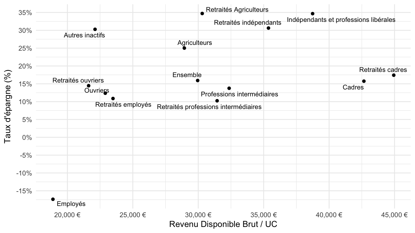
Quintile + age
Taux d’épargne
Code
ip1815 %>%
  filter(sheet == "fig6") %>%
  mutate(classe = case_when(grepl("quintile", type) ~ "Quintiles",
                            grepl(" ans", type) ~ "Age",
                            T ~ "Classe")) %>%
  filter(classe != "Classe") %>%
  ggplot(., aes(x = `Revenu Disponible Brut / UC`, y = 1-`Consommation / UC` / `Revenu Disponible Brut / UC`,color = classe)) + geom_point() +
  theme_minimal() + geom_abline(slope = 1) + ylab("Taux d'épargne (%)") +
  theme(legend.position = c(0.2, 0.8),
        legend.title = element_blank()) +
  theme(axis.text.x = element_text(angle = 45, vjust = 1, hjust = 1)) +
  scale_x_continuous(breaks = seq(0, 100000, 2000),
                     labels = dollar_format(pre = "", su = " €")) +
  scale_y_continuous(breaks = 0.01*seq(-100, 100, 1),
                     labels = percent_format(acc = 1)) +
  geom_text_repel(aes(x = `Revenu Disponible Brut / UC`, y = 1-`Consommation / UC` / `Revenu Disponible Brut / UC`, label = paste0(type, "\nTaux d'épargne: ",  percent(1-`Consommation / UC` / `Revenu Disponible Brut / UC`, acc = 1)), color = classe),
                  fontface ="plain", size = 3) +
  scale_color_manual(values = c("blue", "red"))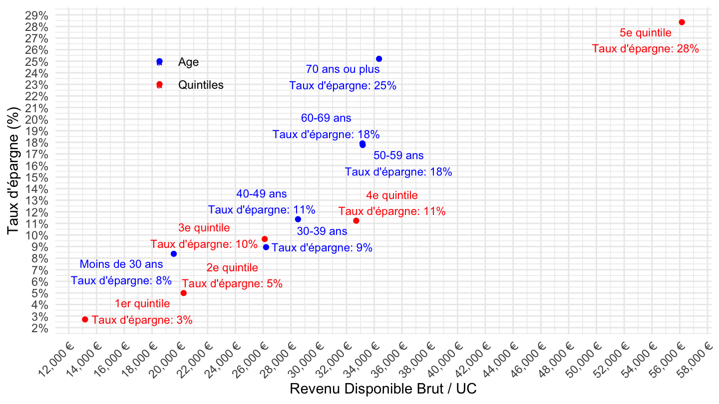
Tous
Table
Code
ip1815 %>%
  filter(sheet == "fig6") %>%
  mutate(classe = case_when(grepl("quintile", type) ~ "Quintiles",
                            grepl(" ans", type) ~ "Age",
                            T ~ "Classe")) %>%
  mutate(`Epargne / UC` = `Revenu Disponible Brut / UC`-`Consommation / UC`,
         `taux d'épargne` = round(100*(1-`Consommation / UC` / `Revenu Disponible Brut / UC`), 1)) %>%
  select(-sheet) %>%
print_table_conditional()| type | Consommation / UC | Revenu Disponible Brut / UC | classe | Epargne / UC | taux d'épargne |
|---|---|---|---|---|---|
| 1er quintile | 12816 | 13173 | Quintiles | 357 | 2.7 |
| 2e quintile | 19262 | 20273 | Quintiles | 1011 | 5.0 |
| 3e quintile | 23592 | 26112 | Quintiles | 2520 | 9.7 |
| 4e quintile | 29029 | 32702 | Quintiles | 3673 | 11.2 |
| 5e quintile | 40222 | 56153 | Quintiles | 15931 | 28.4 |
| Moins de 30 ans | 17924 | 19562 | Age | 1638 | 8.4 |
| 30-39 ans | 23865 | 26210 | Age | 2345 | 8.9 |
| 40-49 ans | 25270 | 28509 | Age | 3239 | 11.4 |
| 50-59 ans | 27276 | 33169 | Age | 5893 | 17.8 |
| 60-69 ans | 27215 | 33150 | Age | 5935 | 17.9 |
| 70 ans ou plus | 25689 | 34346 | Age | 8657 | 25.2 |
| Agriculteurs | 21698 | 28937 | Classe | 7239 | 25.0 |
| Indépendants et professions libérales | 25307 | 38739 | Classe | 13432 | 34.7 |
| Cadres | 35946 | 42659 | Classe | 6713 | 15.7 |
| Professions intermédiaires | 27910 | 32360 | Classe | 4450 | 13.8 |
| Employés | 22178 | 18895 | Classe | -3283 | -17.4 |
| Ouvriers | 20064 | 22894 | Classe | 2830 | 12.4 |
| Retraités Agriculteurs | 19783 | 30303 | Classe | 10520 | 34.7 |
| Retraités indépendants | 24533 | 35366 | Classe | 10833 | 30.6 |
| Retraités cadres | 37112 | 44940 | Classe | 7828 | 17.4 |
| Retraités professions intermédiaires | 28222 | 31441 | Classe | 3219 | 10.2 |
| Retraités employés | 20931 | 23485 | Classe | 2554 | 10.9 |
| Retraités ouvriers | 18495 | 21622 | Classe | 3127 | 14.5 |
| Autres inactifs | 15417 | 22113 | Classe | 6696 | 30.3 |
| Ensemble | 25184 | 29954 | Classe | 4770 | 15.9 |
Fonction de consommation
Code
ip1815 %>%
  filter(sheet == "fig6") %>%
  mutate(classe = case_when(grepl("quintile", type) ~ "Quintiles",
                            grepl(" ans", type) ~ "Age",
                            T ~ "Classe")) %>%
  ggplot(., aes(x = `Revenu Disponible Brut / UC`, y = `Consommation / UC`, color = classe)) + geom_point() +
  theme_minimal() + geom_abline(slope = 1) +
  theme(legend.position = c(0.7, 0.2),
        legend.title = element_blank()) +
  scale_x_continuous(breaks = seq(0, 100000, 5000),
                     labels = dollar_format(pre = "", su = " €")) +
  scale_y_continuous(breaks = seq(0, 100000, 5000),
                     labels = dollar_format(pre = "", su = " €")) +
  geom_text_repel(aes(x = `Revenu Disponible Brut / UC`, y = `Consommation / UC`, label = type, color = classe),
                  fontface ="plain", size = 3)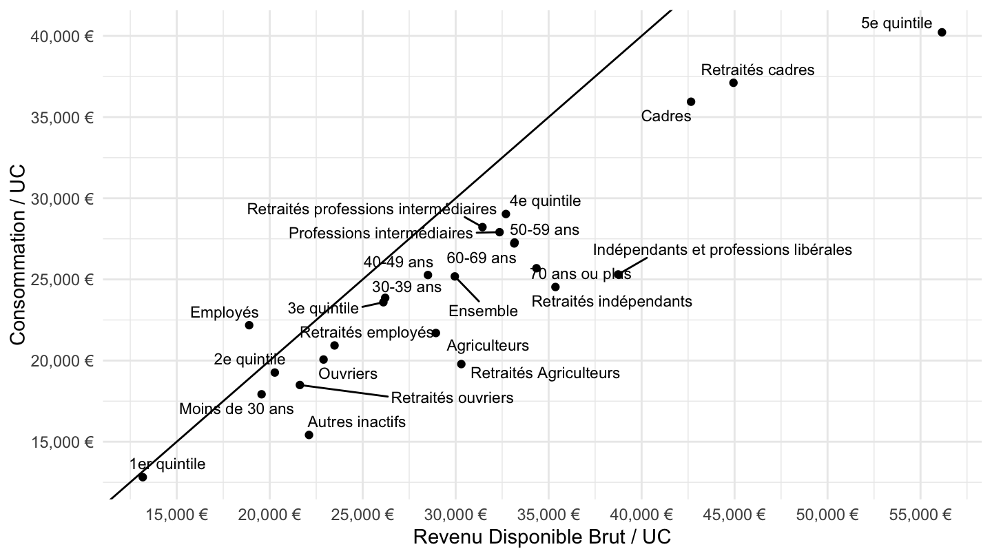
Fonction d’épargne
Code
ip1815 %>%
  filter(sheet == "fig6") %>%
  mutate(classe = case_when(grepl("quintile", type) ~ "Quintiles",
                            grepl(" ans", type) ~ "Age",
                            T ~ "Classe")) %>%
  mutate(`Epargne / UC` = `Revenu Disponible Brut / UC` - `Consommation / UC`) %>%
  ggplot(., aes(x = `Revenu Disponible Brut / UC`, y = `Epargne / UC`, color = classe)) + geom_point() +
  theme_minimal() + geom_abline(slope = 1) +
  theme(legend.position = c(0.7, 0.2),
        legend.title = element_blank()) +
  scale_x_continuous(breaks = seq(0, 100000, 5000),
                     labels = dollar_format(pre = "", su = " €")) +
  scale_y_continuous(breaks = seq(0, 100000, 5000),
                     labels = dollar_format(pre = "", su = " €")) +
  geom_text_repel(aes(x = `Revenu Disponible Brut / UC`, y = `Epargne / UC`, label = type, color = classe),
                  fontface ="plain", size = 3)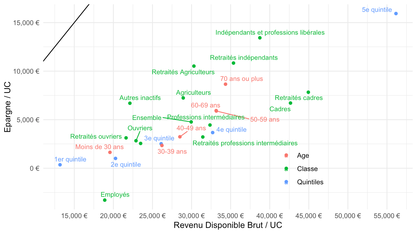
Taux d’épargne
Code
ip1815 %>%
  filter(sheet == "fig6") %>%
  mutate(classe = case_when(grepl("quintile", type) ~ "Quintiles",
                            grepl(" ans", type) ~ "Age",
                            T ~ "Classe")) %>%
  ggplot(., aes(x = `Revenu Disponible Brut / UC`, y = 1-`Consommation / UC` / `Revenu Disponible Brut / UC`,color = classe)) + geom_point() +
  theme_minimal() + geom_abline(slope = 1) + ylab("Taux d'épargne (%)") +
  theme(legend.position = c(0.7, 0.2),
        legend.title = element_blank()) +
  scale_x_continuous(breaks = seq(0, 100000, 5000),
                     labels = dollar_format(pre = "", su = " €")) +
  scale_y_continuous(breaks = 0.01*seq(-100, 100, 5),
                     labels = percent_format(acc = 1)) +
  geom_text_repel(aes(x = `Revenu Disponible Brut / UC`, y = 1-`Consommation / UC` / `Revenu Disponible Brut / UC`, label = type, color = classe),
                  fontface ="plain", size = 3)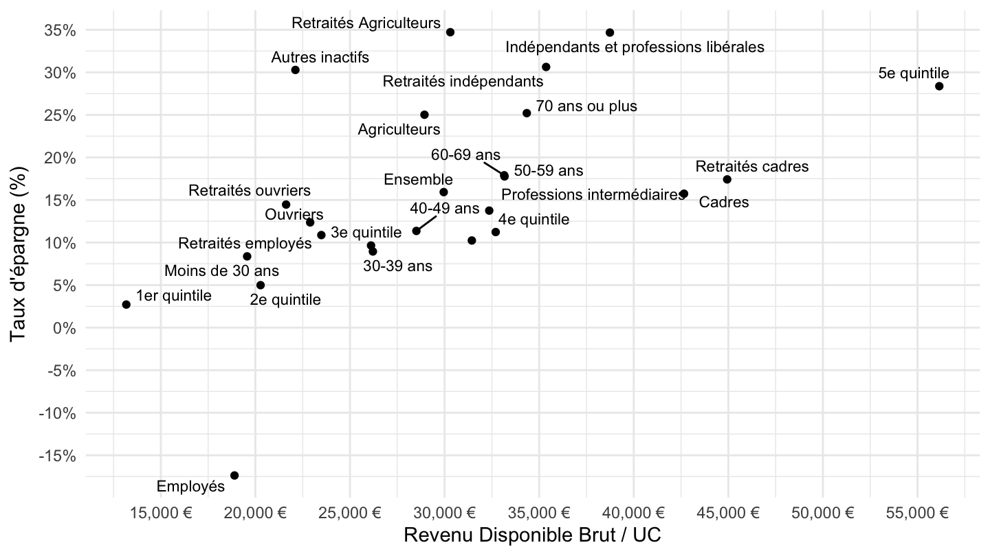
Données Insee Première
Composition de la dépense de consommation
Code
ig_b("insee", "ip1815", "bind")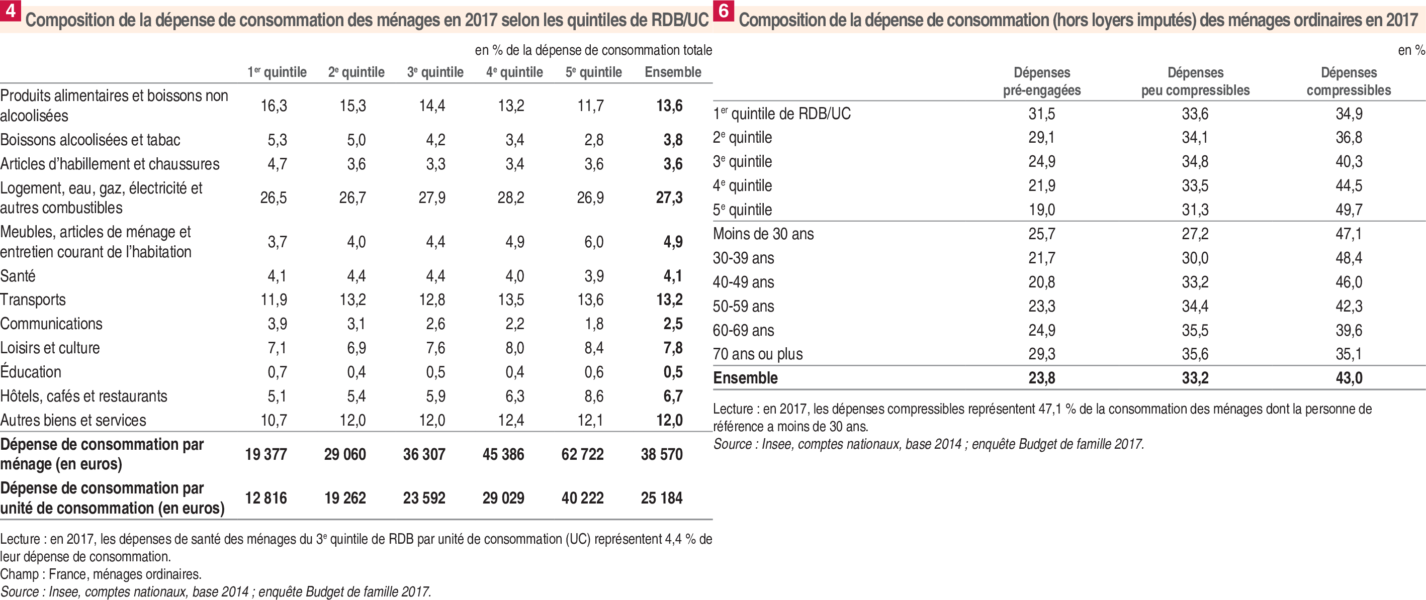
Taux d’épargne par quintile
Code
ig_b("insee", "ip1815", "fig5")