Wage
Data - Fred
Info
LAST_COMPILE
| LAST_COMPILE |
|---|
| 2026-07-24 |
Last
| date | Nobs |
|---|---|
| 2026-06-01 | 5 |
variable
Code
wage %>%
  left_join(variable,  by = "variable") %>%
  group_by(variable, Variable) %>%
  arrange(date) %>%
  summarise(Nobs = n(),
            first = first(date),
            last = last(date)) %>%
  arrange(-Nobs) %>%
  {if (is_html_output()) datatable(., filter = 'top', rownames = F) else .}
Employment Cost Index (Wages)
ECIWAG, ECICONWAG, CPIAUCSL
All
Code
wage %>%
  bind_rows(cpi) %>%
  filter(variable %in% c("ECIWAG", "ECICONWAG", "CPIAUCSL")) %>%
  filter(month(date) %in% c(1, 4, 7, 10),
         !is.na(value)) %>%
  select(date, variable, value) %>%
  group_by(variable) %>%
  filter(date >= as.Date("2001-01-01")) %>%
  arrange(date) %>%
  mutate(value_d1 = value/lag(value, 4) - 1) %>%
  na.omit %>%
  ggplot(.) + geom_line(aes(x = date, y = value_d1, color = variable)) + theme_minimal() +
  scale_x_date(breaks = "12 months",
               labels = date_format("%b %Y")) +
  scale_y_continuous(breaks = 0.01*seq(-60, 60, 0.5),
                     labels = scales::percent_format(accuracy = .1)) +
  xlab("") + ylab("ECI Inflation (%)") +
  theme(legend.position = c(0.4, 0.8),
        legend.title = element_blank(),
        axis.text.x = element_text(angle = 45, vjust = 1, hjust = 1))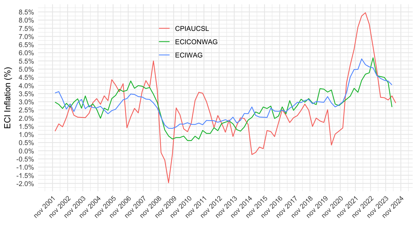
2010-
Code
wage %>%
  bind_rows(cpi) %>%
  filter(variable %in% c("ECIWAG", "ECICONWAG", "CPIAUCSL")) %>%
  filter(month(date) %in% c(1, 4, 7, 10),
         !is.na(value)) %>%
  select(date, variable, value) %>%
  group_by(variable) %>%
  filter(date >= as.Date("2010-01-01")) %>%
  arrange(date) %>%
  mutate(value_d1 = value/lag(value, 4) - 1) %>%
  na.omit %>%
  ggplot(.) + geom_line(aes(x = date, y = value_d1, color = variable)) + theme_minimal() +
  scale_x_date(breaks = "12 months",
               labels = date_format("%b %Y")) +
  scale_y_continuous(breaks = 0.01*seq(-60, 60, 0.5),
                     labels = scales::percent_format(accuracy = .1)) +
  xlab("") + ylab("ECI Inflation (%)") +
  theme(legend.position = c(0.4, 0.8),
        legend.title = element_blank(),
        axis.text.x = element_text(angle = 45, vjust = 1, hjust = 1))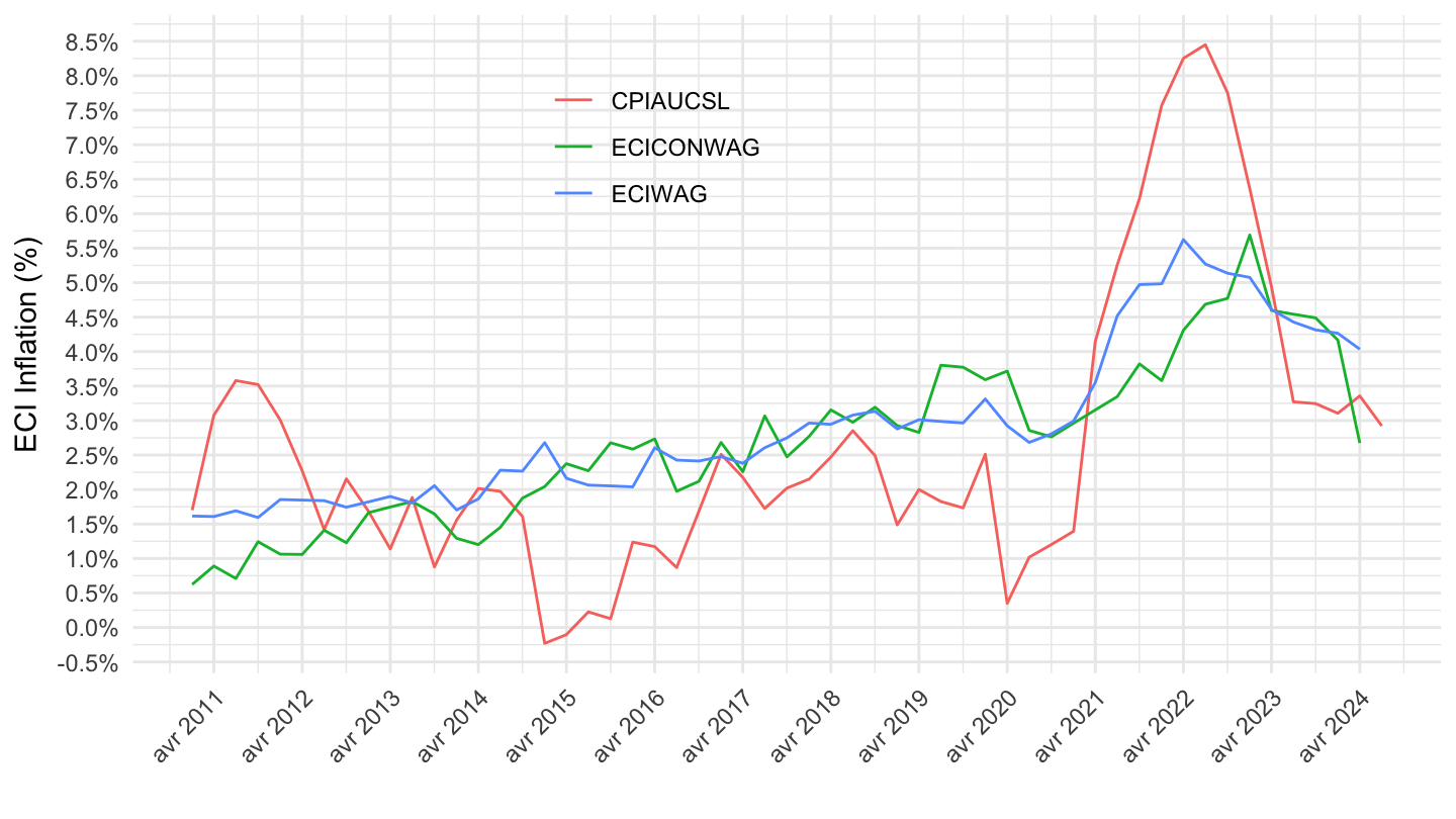
2017-
Code
wage %>%
  bind_rows(cpi) %>%
  filter(variable %in% c("ECIWAG", "ECICONWAG", "CPIAUCSL")) %>%
  filter(month(date) %in% c(1, 4, 7, 10),
         !is.na(value)) %>%
  select(date, variable, value) %>%
  group_by(variable) %>%
  filter(date >= as.Date("2017-01-01")) %>%
  arrange(date) %>%
  mutate(value_d1 = value/lag(value, 4) - 1) %>%
  na.omit %>%
  ggplot(.) + geom_line(aes(x = date, y = value_d1, color = variable)) + theme_minimal() +
  scale_x_date(breaks = "3 months",
               labels = date_format("%b %Y")) +
  scale_y_continuous(breaks = 0.01*seq(-60, 60, 0.5),
                     labels = scales::percent_format(accuracy = .1)) +
  xlab("") + ylab("ECI Inflation (%)") +
  theme(legend.position = c(0.4, 0.8),
        legend.title = element_blank(),
        axis.text.x = element_text(angle = 45, vjust = 1, hjust = 1))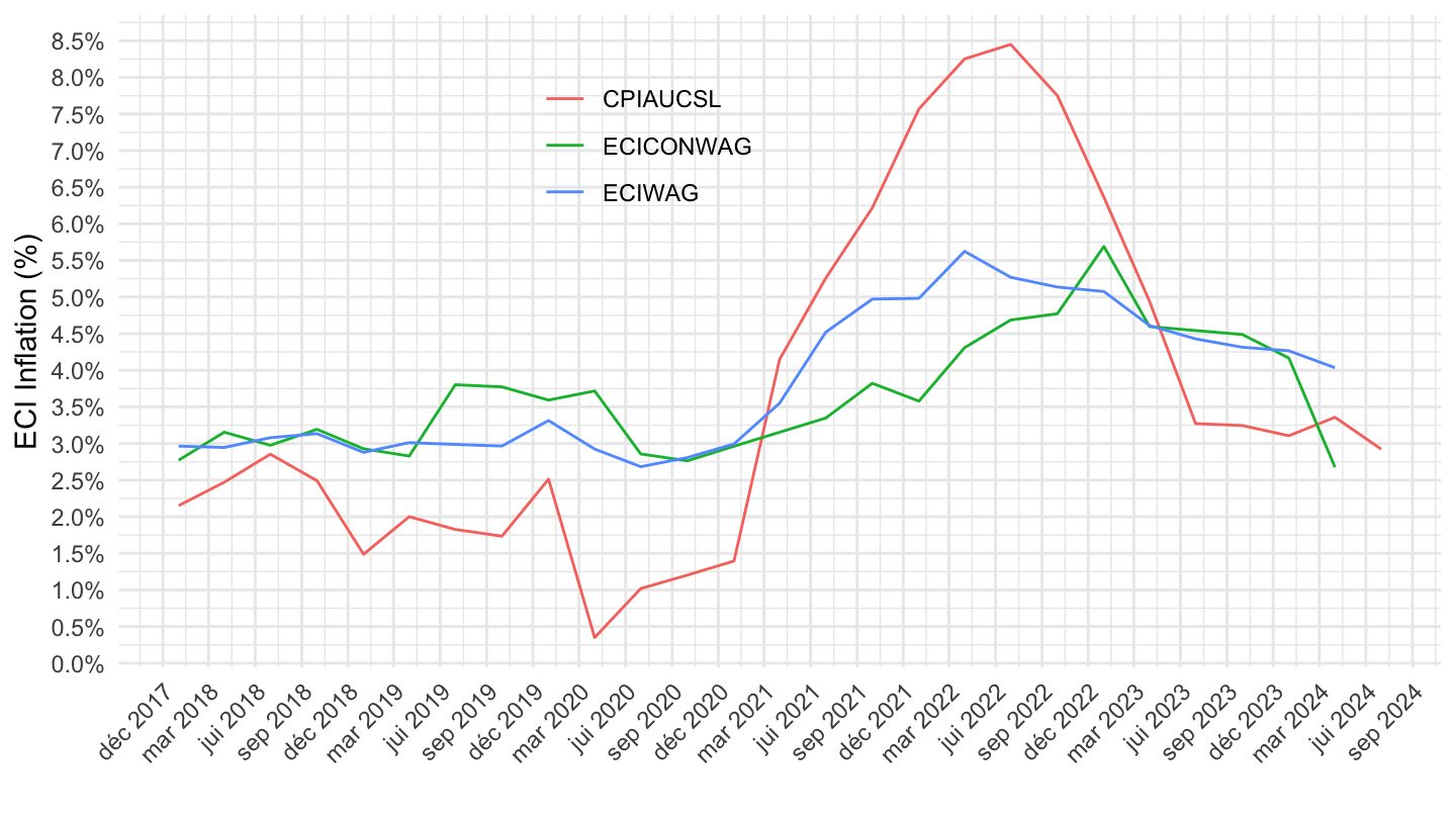
ECIWAG, ECICONWAG
All
Code
wage %>%
  filter(variable %in% c("ECIWAG", "ECICONWAG")) %>%
  select(date, variable, value) %>%
  group_by(variable) %>%
  arrange(date) %>%
  mutate(value = value/lag(value, 4) - 1) %>%
  left_join(variable, by = "variable") %>%
  na.omit %>%
  ggplot(.) + geom_line(aes(x = date, y = value, color = Variable)) + theme_minimal() +
  scale_x_date(breaks = "12 months",
               labels = date_format("%b %Y")) +
  scale_y_continuous(breaks = 0.01*seq(-60, 60, 0.5),
                     labels = scales::percent_format(accuracy = .1)) +
  xlab("") + ylab("ECI Inflation (%)") +
  theme(legend.position = c(0.4, 0.8),
        legend.title = element_blank(),
        axis.text.x = element_text(angle = 45, vjust = 1, hjust = 1))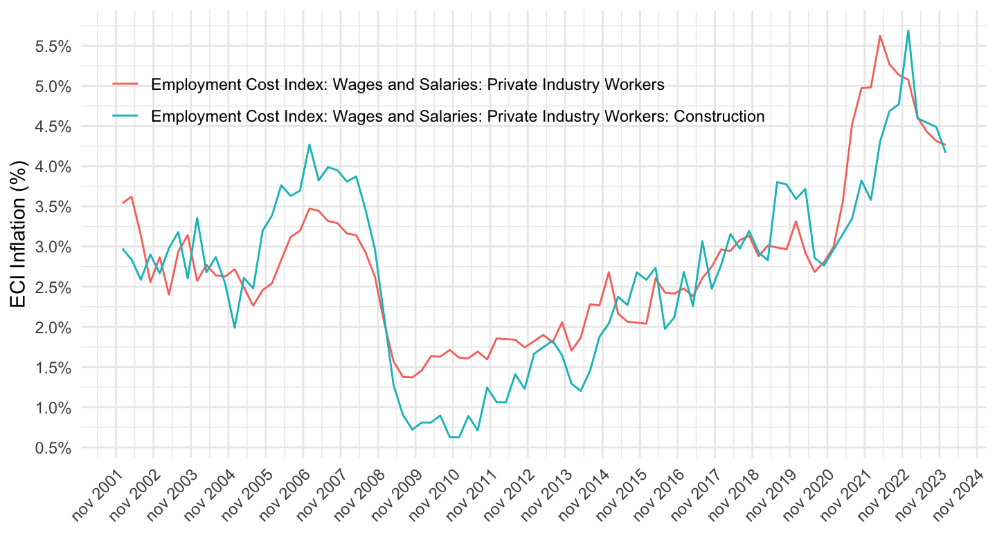
2010-
Code
wage %>%
  filter(variable %in% c("ECIWAG", "ECICONWAG")) %>%
  select(date, variable, value) %>%
  group_by(variable) %>%
  arrange(date) %>%
  mutate(value = value/lag(value, 4) - 1) %>%
  filter(date >= as.Date("2010-01-01")) %>%
  left_join(variable, by = "variable") %>%
  na.omit %>%
  ggplot(.) + geom_line(aes(x = date, y = value, color = Variable)) + theme_minimal() +
  scale_x_date(breaks = "12 months",
               labels = date_format("%b %Y")) +
  scale_y_continuous(breaks = 0.01*seq(-60, 60, 0.5),
                     labels = scales::percent_format(accuracy = .1)) +
  xlab("") + ylab("ECI Inflation (%)") +
  theme(legend.position = c(0.4, 0.8),
        legend.title = element_blank(),
        axis.text.x = element_text(angle = 45, vjust = 1, hjust = 1))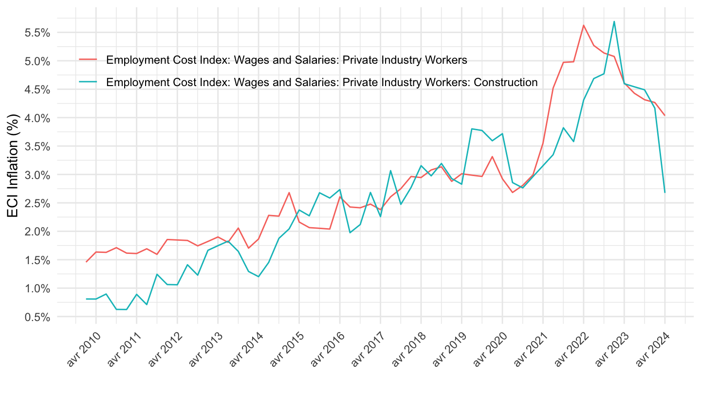
2019-
Code
wage %>%
  filter(variable %in% c("ECIWAG", "ECICONWAG")) %>%
  select(date, variable, value) %>%
  group_by(variable) %>%
  arrange(date) %>%
  mutate(value = value/lag(value, 4) - 1) %>%
  filter(date >= as.Date("2019-01-01")) %>%
  left_join(variable, by = "variable") %>%
  na.omit %>%
  ggplot(.) + geom_line(aes(x = date, y = value, color = Variable)) + theme_minimal() +
  scale_x_date(breaks = "3 months",
               labels = date_format("%b %Y")) +
  scale_y_continuous(breaks = 0.01*seq(-60, 60, 0.5),
                     labels = scales::percent_format(accuracy = .1)) +
  xlab("") + ylab("ECI Inflation (%)") +
  theme(legend.position = c(0.4, 0.8),
        legend.title = element_blank(),
        axis.text.x = element_text(angle = 45, vjust = 1, hjust = 1))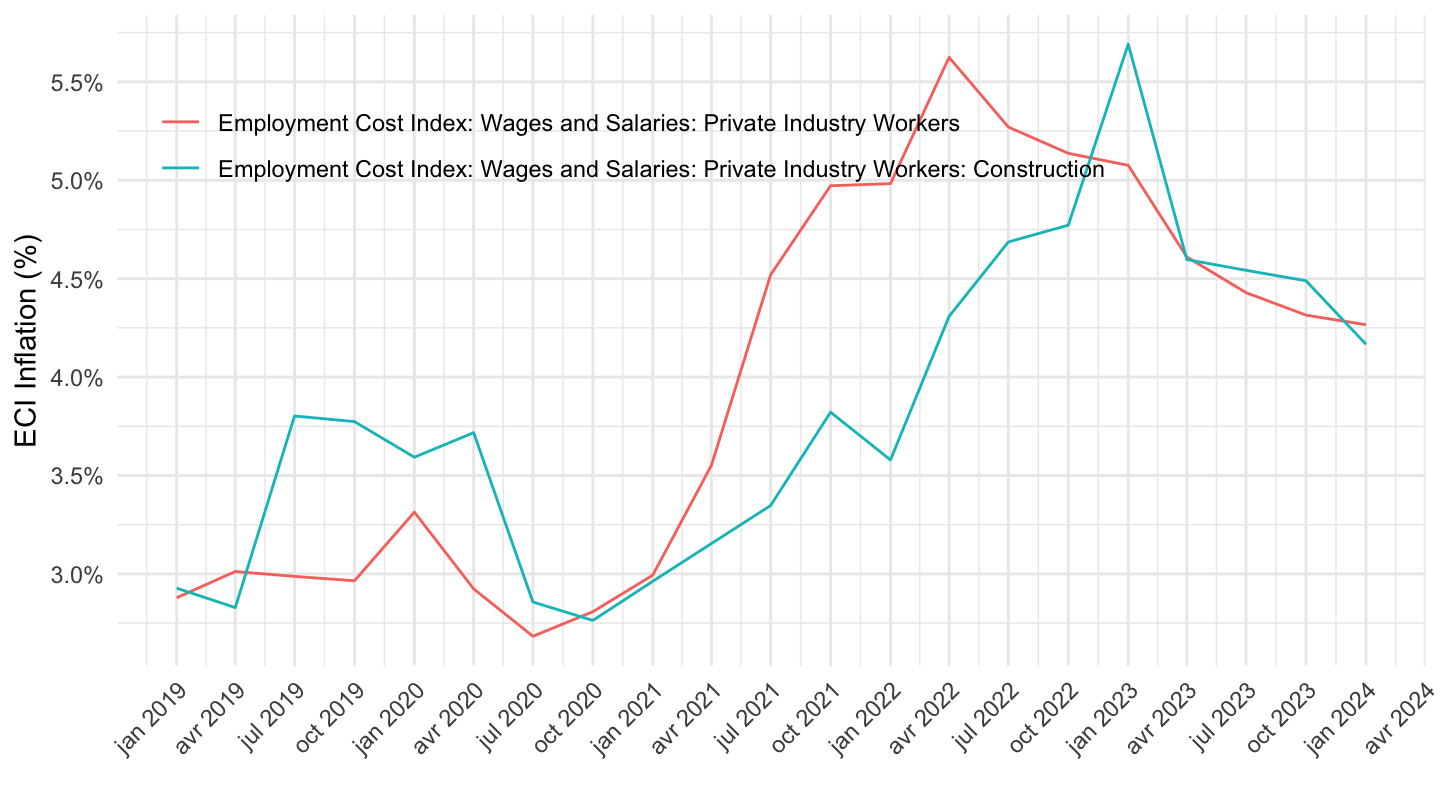
Real Average Hourly Earnings of All Employees, Total Private - CES3000000008
Index
All
Code
wage %>%
  bind_rows(cpi) %>%
  filter(variable %in% c("CPIAUCSL", "CES3000000008")) %>%
  select(date, variable, value) %>%
  unique %>%
  spread(variable, value) %>%
  mutate(CES3000000008_real = CES3000000008/CPIAUCSL) %>%
  filter(!is.na(CES3000000008_real)) %>%
  mutate(CES3000000008_real = 100*CES3000000008_real/CES3000000008_real[date == as.Date("1972-01-01")]) %>%
  ggplot(.) + geom_line(aes(x = date, y = CES3000000008_real)) +
  ylab("Real Wages") + xlab("") + theme_minimal() +
  scale_y_log10(breaks = seq(0, 200, 5)) +
  scale_x_date(breaks = as.Date(paste0(seq(1942, 2100, 5), "-01-01")),
               labels = date_format("%Y")) +
  geom_hline(yintercept = 100, linetype = "dashed", color = "red")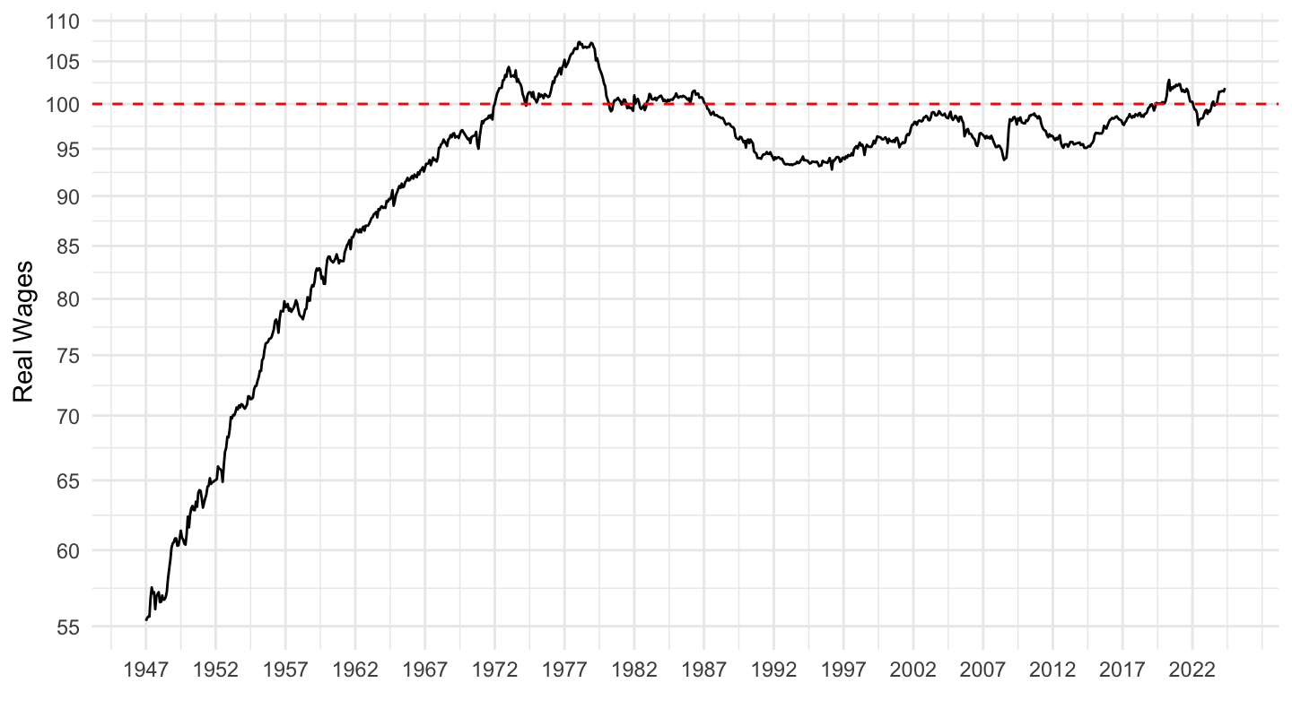
1970-
Code
wage %>%
  bind_rows(cpi) %>%
  filter(variable %in% c("CPIAUCSL", "CES3000000008")) %>%
  select(date, variable, value) %>%
  filter(date >= as.Date("1970-01-01")) %>%
  unique %>%
  spread(variable, value) %>%
  mutate(CES3000000008_real = CES3000000008/CPIAUCSL) %>%
  filter(!is.na(CES3000000008_real)) %>%
  mutate(CES3000000008_real = 100*CES3000000008_real/CES3000000008_real[1]) %>%
  ggplot(.) + geom_line(aes(x = date, y = CES3000000008_real)) +
  ylab("Real Wages") + xlab("") + theme_minimal() +
  scale_y_log10(breaks = seq(0, 200, 2)) +
  scale_x_date(breaks = as.Date(paste0(seq(1940, 2100, 5), "-01-01")),
               labels = date_format("%Y")) +
  geom_hline(yintercept = 100, linetype = "dashed", color = "red")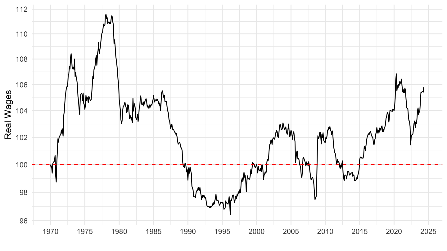
Round Stagflation: 1960-1980
Code
wage %>%
  bind_rows(cpi) %>%
  filter(variable %in% c("CPIAUCSL", "CES3000000008")) %>%
  select(date, variable, value) %>%
  filter(date >= as.Date("1960-01-01"),
         date <= as.Date("1980-01-01")) %>%
  unique %>%
  spread(variable, value) %>%
  mutate(CES3000000008_real = CES3000000008/CPIAUCSL) %>%
  filter(!is.na(CES3000000008_real)) %>%
  mutate(CES3000000008_real = 100*CES3000000008_real/CES3000000008_real[1]) %>%
  ggplot(.) + geom_line(aes(x = date, y = CES3000000008_real)) +
  ylab("Real Wages") + xlab("") + theme_minimal() +
  scale_y_log10(breaks = seq(0, 200, 2)) +
  scale_x_date(breaks = as.Date(paste0(seq(1960, 2100, 2), "-01-01")),
               labels = date_format("%Y")) +
  geom_hline(yintercept = 100, linetype = "dashed", color = "red")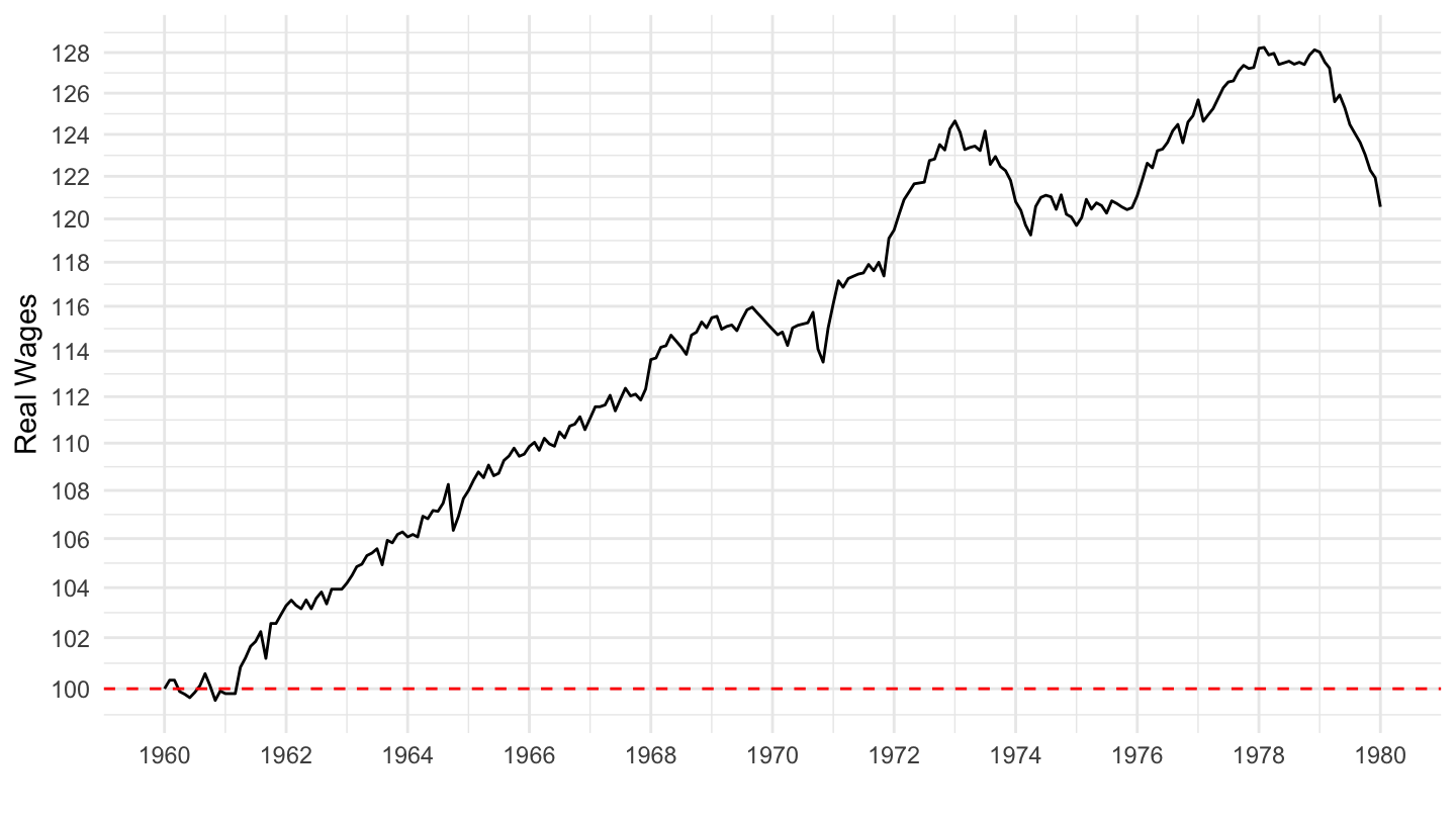
1972-
Code
wage %>%
  bind_rows(cpi) %>%
  filter(variable %in% c("CPIAUCSL", "CES3000000008")) %>%
  select(date, variable, value) %>%
  filter(date >= as.Date("1972-01-01")) %>%
  unique %>%
  spread(variable, value) %>%
  mutate(CES3000000008_real = CES3000000008/CPIAUCSL) %>%
  filter(!is.na(CES3000000008_real)) %>%
  mutate(CES3000000008_real = 100*CES3000000008_real/CES3000000008_real[1]) %>%
  ggplot(.) + geom_line(aes(x = date, y = CES3000000008_real)) +
  ylab("Real Wages") + xlab("") + theme_minimal() +
  scale_y_log10(breaks = seq(0, 200, 2)) +
  scale_x_date(breaks = as.Date(paste0(seq(1972, 2100, 5), "-01-01")),
               labels = date_format("%Y")) +
  geom_hline(yintercept = 100, linetype = "dashed", color = "red")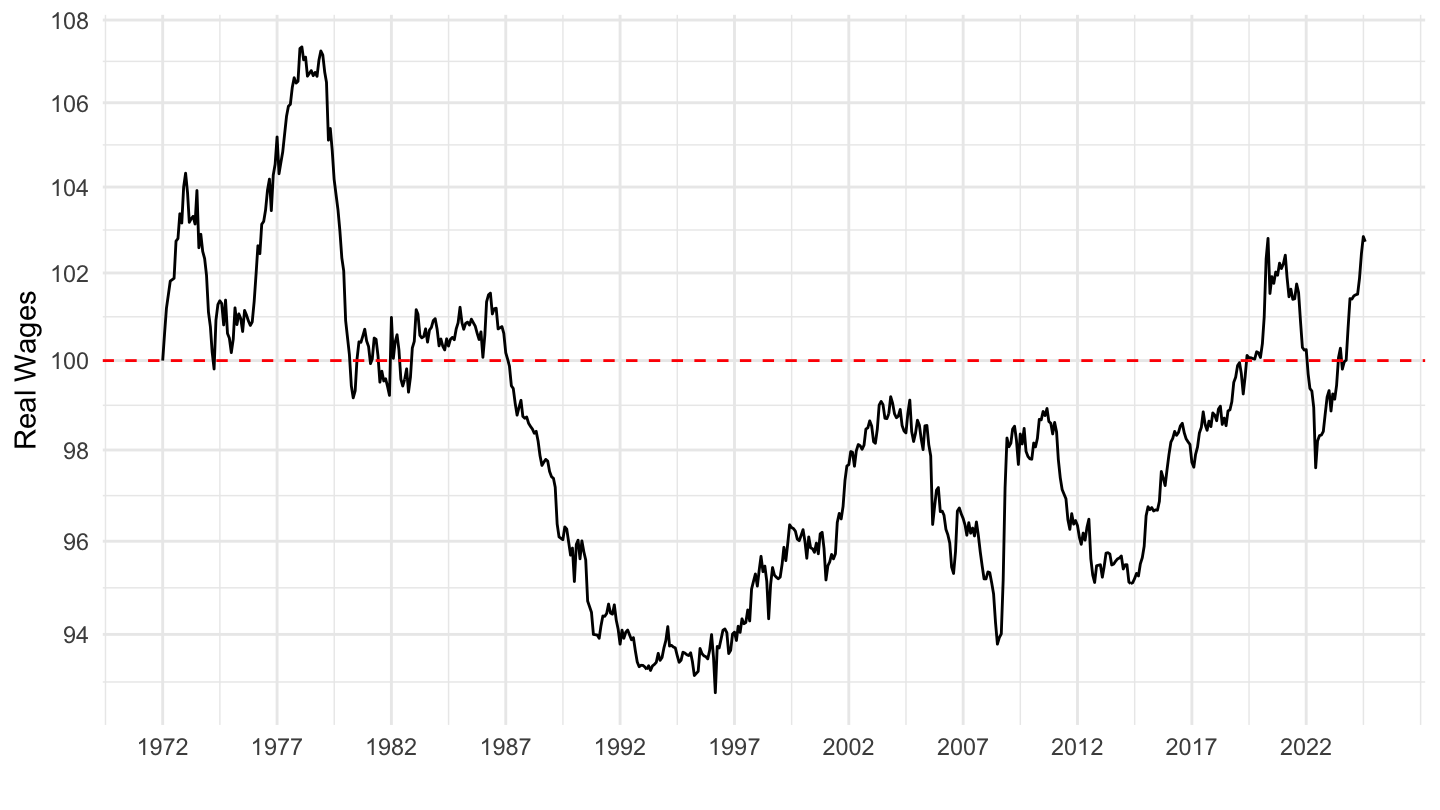
1995-
Code
wage %>%
  bind_rows(cpi) %>%
  filter(variable %in% c("CPIAUCSL", "CES3000000008")) %>%
  select(date, variable, value) %>%
  filter(date >= as.Date("1995-01-01")) %>%
  unique %>%
  spread(variable, value) %>%
  mutate(CES3000000008_real = CES3000000008/CPIAUCSL) %>%
  filter(!is.na(CES3000000008_real)) %>%
  mutate(CES3000000008_real = 100*CES3000000008_real/CES3000000008_real[1]) %>%
  ggplot(.) + geom_line(aes(x = date, y = CES3000000008_real)) +
  ylab("Real Wages") + xlab("") + theme_minimal() +
  scale_y_log10(breaks = seq(0, 200, 2)) +
  scale_x_date(breaks = as.Date(paste0(seq(1940, 2100, 5), "-01-01")),
               labels = date_format("%Y"))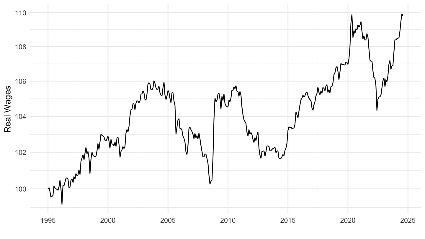
2002-
Code
wage %>%
  bind_rows(cpi) %>%
  filter(variable %in% c("CPIAUCSL", "CES3000000008")) %>%
  select(date, variable, value) %>%
  filter(date >= as.Date("2002-01-01")) %>%
  unique %>%
  spread(variable, value) %>%
  mutate(CES3000000008_real = CES3000000008/CPIAUCSL) %>%
  filter(!is.na(CES3000000008_real)) %>%
  mutate(CES3000000008_real = 100*CES3000000008_real/CES3000000008_real[1]) %>%
  ggplot(.) + geom_line(aes(x = date, y = CES3000000008_real)) +
  ylab("Real Wages") + xlab("") + theme_minimal() +
  scale_y_log10(breaks = seq(0, 200, 2)) +
  scale_x_date(breaks = as.Date(paste0(seq(1940, 2100, 2), "-01-01")),
               labels = date_format("%Y"))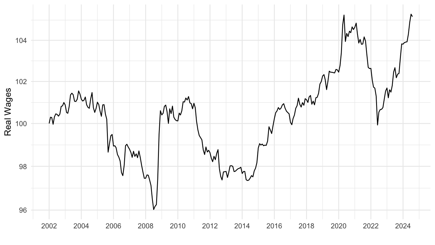
Log
Code
wage %>%
  bind_rows(cpi) %>%
  filter(variable %in% c("CPIAUCSL", "CES0500000003")) %>%
  filter(month(date) == 1) %>%
  select(date, variable, value) %>%
  spread(variable, value) %>%
  mutate(CES0500000003_real = CES0500000003/CPIAUCSL) %>%
  filter(!is.na(CES0500000003_real)) %>%
  mutate(wage_inflation = CES0500000003_real/lag(CES0500000003_real)-1) %>%
  ggplot(.) + ylab("Real Wage Inflation") + xlab("") +
  geom_line(aes(x = date, y = wage_inflation)) +
  scale_y_continuous(breaks = seq(-0.2, 0.4, 0.01),
                     labels = percent_format(acc = 1)) +
  scale_x_date(breaks = as.Date(paste0(seq(1940, 2100, 2), "-01-01")),
               labels = date_format("%Y")) +
  theme_minimal()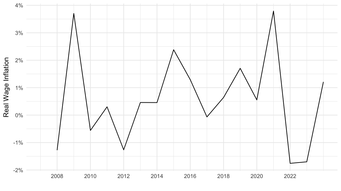
Real Average
Index
All
Code
wage %>%
  bind_rows(cpi) %>%
  filter(variable %in% c("CPIAUCSL", "CES0500000003")) %>%
  select(date, variable, value) %>%
  unique %>%
  spread(variable, value) %>%
  na.omit %>%
  mutate(CES0500000003_real = CES0500000003/CPIAUCSL) %>%
  filter(!is.na(CES0500000003_real)) %>%
  mutate(CES0500000003_real = 100*CES0500000003_real/CES0500000003_real[1]) %>%
  ggplot(.) + geom_line(aes(x = date, y = CES0500000003_real)) +
  ylab("Real Wages") + xlab("") + theme_minimal() +
  scale_y_log10(breaks = seq(0, 200, 2)) +
  scale_x_date(breaks = as.Date(paste0(seq(1942, 2100, 2), "-01-01")),
               labels = date_format("%Y")) +
  geom_hline(yintercept = 100, linetype = "dashed", color = "red")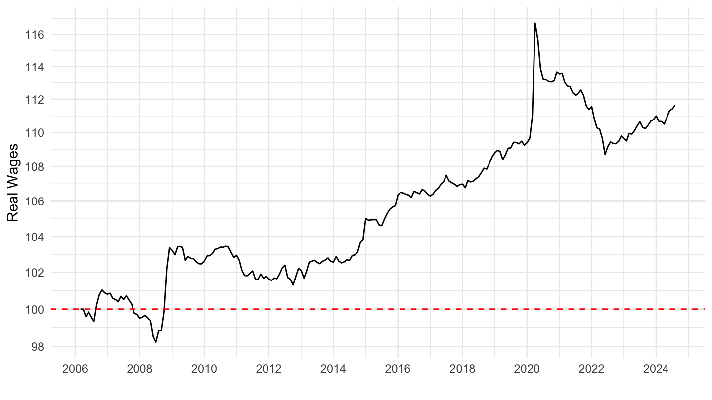
1970-
Code
wage %>%
  bind_rows(cpi) %>%
  filter(variable %in% c("CPIAUCSL", "CES0500000003")) %>%
  select(date, variable, value) %>%
  filter(date >= as.Date("1970-01-01")) %>%
  unique %>%
  spread(variable, value) %>%
  mutate(CES0500000003_real = CES0500000003/CPIAUCSL) %>%
  filter(!is.na(CES0500000003_real)) %>%
  mutate(CES0500000003_real = 100*CES0500000003_real/CES0500000003_real[1]) %>%
  ggplot(.) + geom_line(aes(x = date, y = CES0500000003_real)) +
  ylab("Real Wages") + xlab("") + theme_minimal() +
  scale_y_log10(breaks = seq(0, 200, 2)) +
  scale_x_date(breaks = as.Date(paste0(seq(1940, 2100, 5), "-01-01")),
               labels = date_format("%Y")) +
  geom_hline(yintercept = 100, linetype = "dashed", color = "red")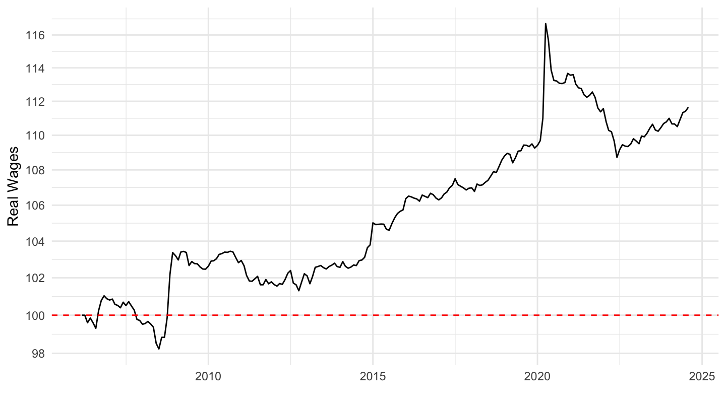
Average Hourly Earnings of All Employees, Total Private - CES0500000003
Index
Code
wage %>%
  filter(variable == "CES0500000003") %>%
  ggplot(.) + geom_line(aes(x = date, y = value)) +
  ylab("Wages") + xlab("") + theme_minimal() +
  scale_y_continuous(breaks = seq(0, 30, 2)) +
  scale_x_date(breaks = as.Date(paste0(seq(1940, 2100, 2), "-01-01")),
               labels = date_format("%Y"))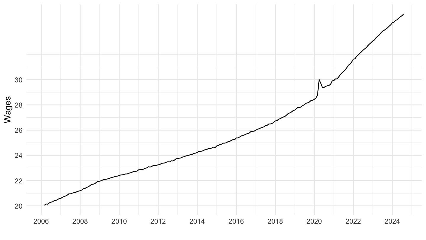
Log
Code
wage %>%
  filter(variable == "CES0500000003") %>%
  mutate(year = year(date),
         month = month(date)) %>%
  filter(month == 1) %>%
  mutate(value_log = log(value),
         wage_inflation = value_log - lag(value_log)) %>%
  ggplot(.) + ylab("Wage Inflation") + xlab("") +
  geom_line(aes(x = date, y = wage_inflation)) +
  scale_y_continuous(breaks = seq(-0.2, 0.4, 0.01),
                     labels = percent_format(acc = 1)) +
  scale_x_date(breaks = as.Date(paste0(seq(1940, 2100, 2), "-01-01")),
               labels = date_format("%Y")) +
  theme_minimal()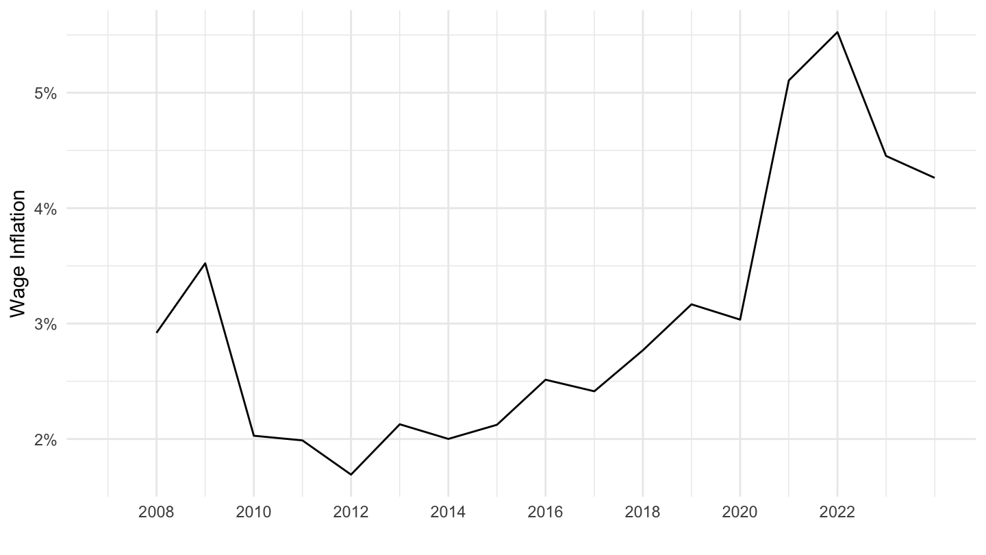
CPIAUCSL
Index
Code
cpi %>%
  filter(variable == "CPIAUCSL") %>%
  ggplot(.) + geom_line(aes(x = date, y = value)) +
  ylab("Wages") + xlab("") + theme_minimal() +
  scale_y_continuous(breaks = seq(0, 30, 2)) +
  scale_x_date(breaks = as.Date(paste0(seq(1940, 2100, 2), "-01-01")),
               labels = date_format("%Y"))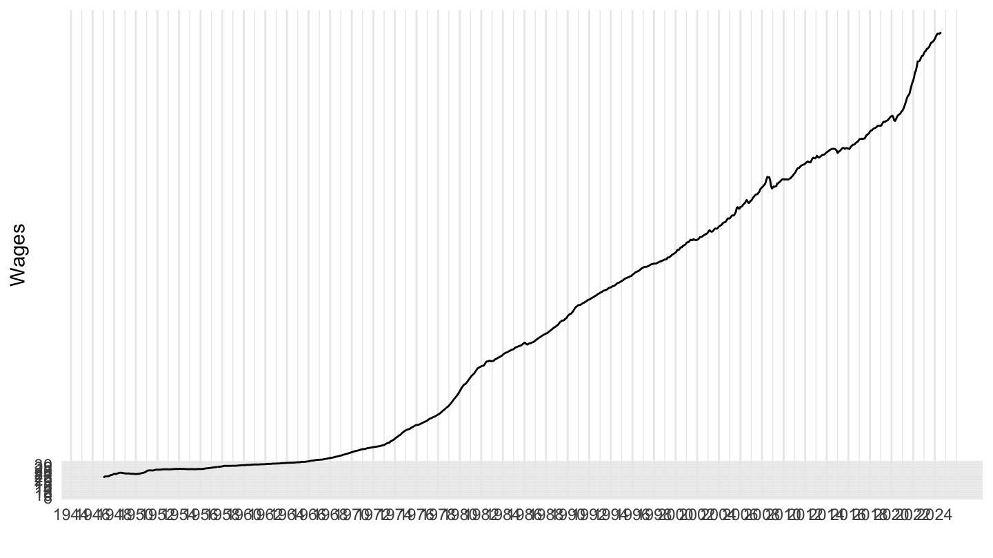
Log
Code
cpi %>%
  filter(variable == "CPIAUCSL") %>%
  mutate(year = year(date),
         month = month(date)) %>%
  filter(month == 1) %>%
  mutate(value_log = log(value),
         wage_inflation = value_log - lag(value_log)) %>%
  filter(date >= as.Date("2008-01-01")) %>%
  ggplot(.) + ylab("Price Inflation") + xlab("") +
  geom_line(aes(x = date, y = wage_inflation)) +
  scale_y_continuous(breaks = seq(-0.2, 0.4, 0.01),
                     labels = percent_format(acc = 1)) +
  scale_x_date(breaks = as.Date(paste0(seq(1940, 2100, 2), "-01-01")),
               labels = date_format("%Y")) +
  theme_minimal()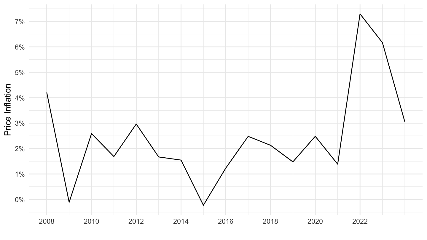
U.S. Index of Manufacturing Wage Rates (07/1922 - 07/1935)
Index
(ref:us-index-CES3000000008) U.S. Index of Manufacturing Wage Rates (07/1922 - 07/1935)
Code
wage %>%
  filter(variable == "CES3000000008") %>%
  ggplot(.) +
  geom_line(aes(x = date, y = value)) +
  ylab("Wages") + xlab("") +
  scale_y_continuous(breaks = seq(0, 30, 2)) +
  scale_x_date(breaks = as.Date(paste0(seq(1940, 2100, 5), "-01-01")),
               labels = date_format("%Y")) +
  theme_minimal()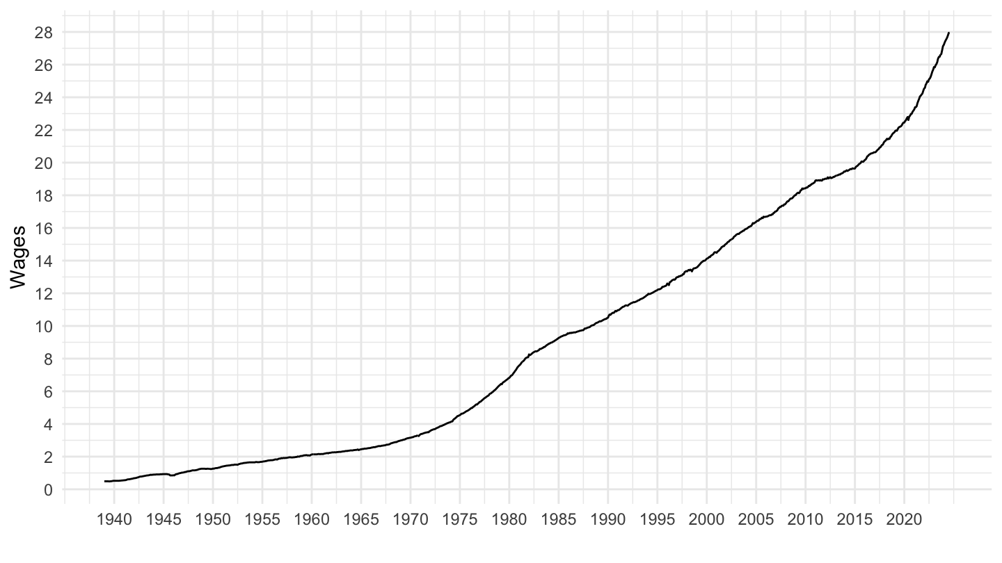
Log
(ref:us-index-CES3000000008-d1ln) U.S. Index of Manufacturing Wage Rates (07/1922 - 07/1935)
Code
wage %>%
  filter(variable == "CES3000000008") %>%
  mutate(year = year(date),
         month = month(date)) %>%
  filter(month == 1) %>%
  mutate(value_log = log(value),
         wage_inflation = value_log - lag(value_log)) %>%
  ggplot(.) + ylab("Wage Inflation") + xlab("") +
  geom_line(aes(x = date, y = wage_inflation)) +
  scale_y_continuous(breaks = seq(-0.2, 0.4, 0.02),
                     labels = percent_format(acc = 1)) +
  scale_x_date(breaks = as.Date(paste0(seq(1940, 2100, 5), "-01-01")),
               labels = date_format("%Y")) +
  theme_minimal()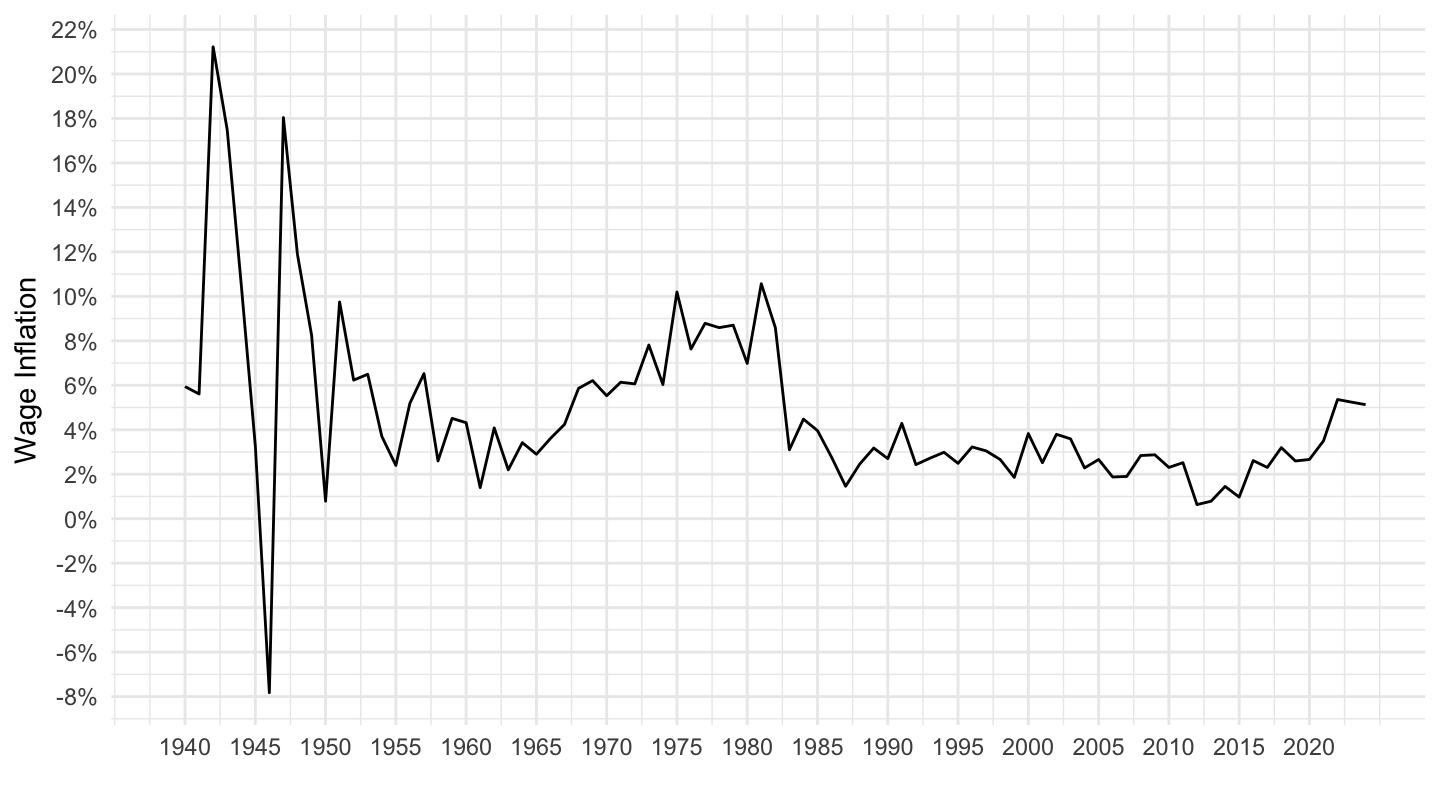
Index of Manufacturing Wages (M0872BUSM234NNBR)
1928-1935
October 29, 1929 (“Black Tuesday”)
Code
wage %>%
  filter(variable == "M0872BUSM234NNBR",
         date >= as.Date("1928-01-01")) %>%
  ggplot(.) +
  geom_line(aes(x = date, y = value)) +
  ylab("Wages") + xlab("") +
  geom_rect(data = nber_recessions,
            aes(xmin = Peak, xmax = Trough, ymin = -Inf, ymax = +Inf),
            fill = viridis(3)[3], alpha = 0.1) +
  scale_y_continuous(breaks = seq(90, 110, 2.5),
                     limits = c(92.5, 110)) +
  scale_x_date(breaks = as.Date(paste0(seq(1928, 1935, 1), "-01-01")),
               labels = date_format("%Y"),
               limits = c(as.Date("1928-01-01"), as.Date("1935-07-01"))) +
  theme_minimal() +
  geom_vline(xintercept = as.Date("1929-10-29"), linetype = "dashed", color = viridis(3)[1]) +
  geom_vline(xintercept = as.Date("1933-04-01"), linetype = "dashed", color = viridis(3)[2])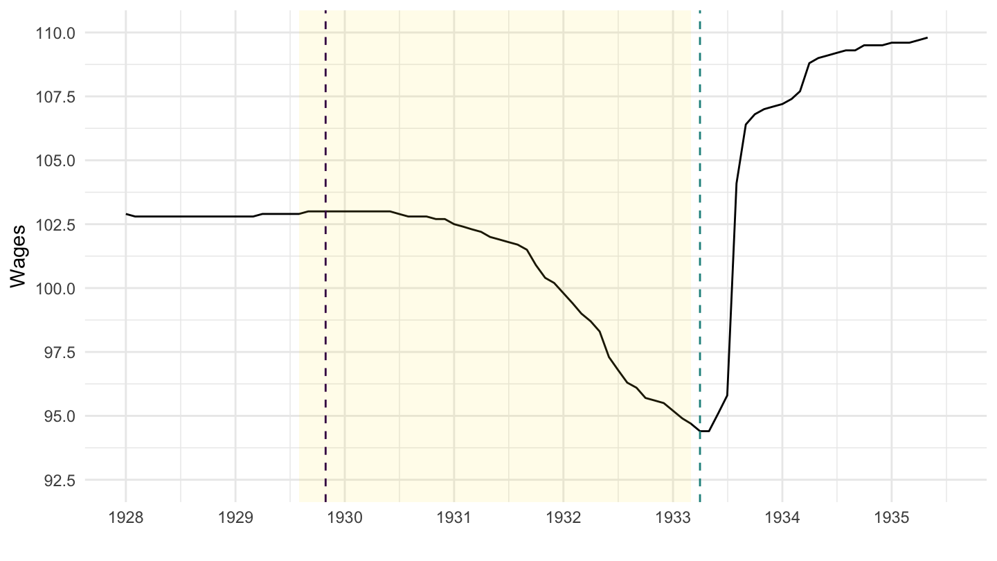
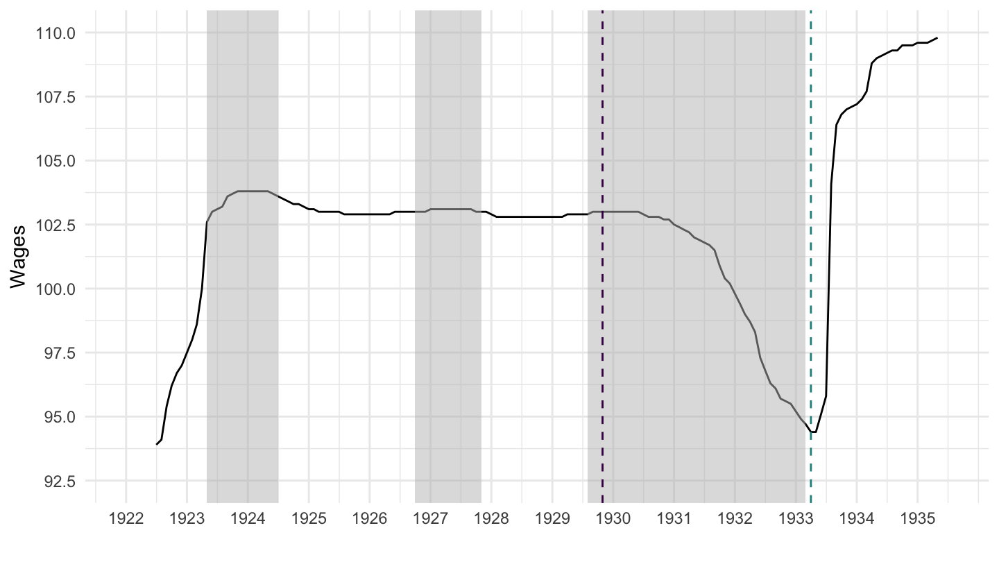
2022-1935
October 29, 1929 (“Black Tuesday”)
(ref:us-index-manuf-wage) U.S. Index of Manufacturing Wage Rates (07/1922 - 07/1935)
Code
wage %>%
  filter(variable == "M0872BUSM234NNBR") %>%
  ggplot(.) +
  geom_line(aes(x = date, y = value)) +
  ylab("Wages") + xlab("") +
  geom_rect(data = nber_recessions,
            aes(xmin = Peak, xmax = Trough, ymin = -Inf, ymax = +Inf),
            fill = 'grey', alpha = 0.5) +
  scale_y_continuous(breaks = seq(90, 110, 2.5),
                     limits = c(92.5, 110)) +
  scale_x_date(breaks = as.Date(paste0(seq(1922, 1935, 1), "-01-01")),
               labels = date_format("%Y"),
               limits = c(as.Date("1922-01-01"), as.Date("1935-07-01"))) +
  theme_minimal() +
  geom_vline(xintercept = as.Date("1929-10-29"), linetype = "dashed", color = viridis(3)[1]) +
  geom_vline(xintercept = as.Date("1933-04-01"), linetype = "dashed", color = viridis(3)[2])