Labour cost index by NACE Rev. 2 activity - nominal value, quarterly data
Data - Eurostat
Info
Last observation: Quarterly: 2026Q1 (N = 27,330)
First observation: Quarterly: 1996Q1 (N = 430)
Last data update: 23 jul 2026, 22:31. Last compile: 24 jul 2026, 02:11
Structure
Last
Europe
Code
lc_lci_r2_q %>%
  filter(geo == "EA20",
         unit != "I20") %>%
  filter(time == max(time)) %>%
  mutate(variable = paste0(s_adj, " - ", unit)) %>%
  select(-unit, -s_adj) %>%
  spread(variable, values) %>%
  select_if(~ n_distinct(.) > 1) %>%
  print_table_conditional()
France
Code
lc_lci_r2_q %>%
  filter(geo == "FR",
         unit != "I20") %>%
  filter(time == max(time)) %>%
  mutate(variable = paste0(s_adj, " - ", unit)) %>%
  select(-unit, -s_adj) %>%
  spread(variable, values) %>%
  select_if(~ n_distinct(.) > 1) %>%
  print_table_conditional()
Germany
Code
lc_lci_r2_q %>%
  filter(geo == "DE",
         unit != "I20") %>%
  filter(time == max(time)) %>%
  mutate(variable = paste0(s_adj, " - ", unit)) %>%
  select(-unit, -s_adj) %>%
  spread(variable, values) %>%
  select_if(~ n_distinct(.) > 1) %>%
  print_table_conditional()
Indices
France
All
Nominal
Code
lc_lci_r2_q %>%
  filter(nace_r2 == "B-S",
         unit == "I20",
         s_adj == "SCA",
         geo %in% c("FR")) %>%
  quarter_to_date %>%


  left_join(colors, by = c("Geo" = "country")) %>%
  group_by(Lcstruct) %>%
  arrange(date) %>%
  mutate(values = 100*values/values[1]) %>%
  ggplot(.) + geom_line(aes(x = date, y = values, color = Lcstruct)) +
  theme_minimal() + xlab("") + ylab("") +
  scale_x_date(breaks = seq(1960, 2100, 2) %>% paste0("-01-01") %>% as.Date,
               labels = date_format("%Y")) +
  scale_y_log10(breaks = seq(80, 200, 5)) +
  theme(legend.position = c(0.45, 0.90),
        legend.title = element_blank())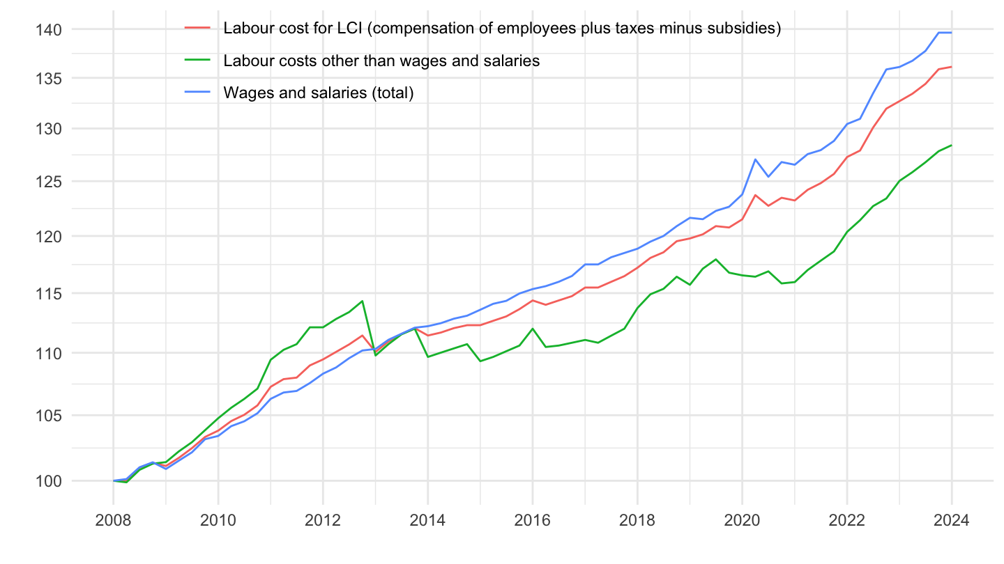
2017T2-
Code
lc_lci_r2_q %>%
  filter(nace_r2 == "B-S",
         unit == "I20",
         s_adj == "SCA",
         geo %in% c("FR")) %>%
  quarter_to_date %>%
  filter(date >= as.Date("2017-04-01")) %>%


  left_join(colors, by = c("Geo" = "country")) %>%
  group_by(Lcstruct) %>%
  arrange(date) %>%
  mutate(values = 100*values/values[1]) %>%
  ggplot(.) + geom_line(aes(x = date, y = values, color = Lcstruct)) +
  theme_minimal() + xlab("") + ylab("") +
  scale_x_date(breaks = seq(1960, 2100, 1) %>% paste0("-01-01") %>% as.Date,
               labels = date_format("%Y")) +
  scale_y_log10(breaks = seq(80, 200, 5)) +
  theme(legend.position = c(0.45, 0.90),
        legend.title = element_blank()) +
  geom_text(data = . %>%
              filter(date %in% max(date)),
            aes(x = date, y = values, color = Lcstruct, label = round(values, 1)))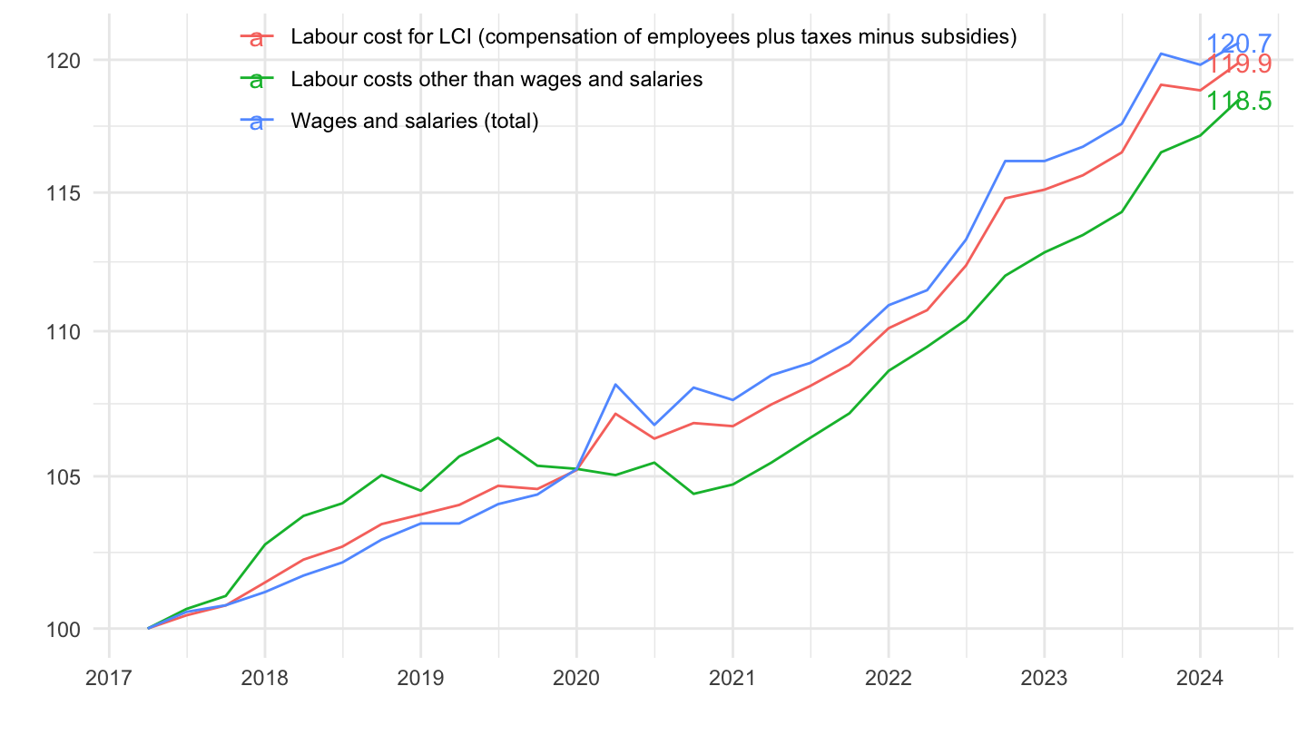
Business
All
Code
lc_lci_r2_q %>%
  filter(nace_r2 == "B-N",
         unit == "I20",
         s_adj == "SCA",
         geo %in% c("FR")) %>%
  quarter_to_date %>%


  left_join(colors, by = c("Geo" = "country")) %>%
  group_by(Lcstruct) %>%
  arrange(date) %>%
  mutate(values = 100*values/values[1]) %>%
  ggplot(.) + geom_line(aes(x = date, y = values, color = Lcstruct)) +
  theme_minimal() + xlab("") + ylab("") +
  scale_x_date(breaks = seq(1960, 2100, 2) %>% paste0("-01-01") %>% as.Date,
               labels = date_format("%Y")) +
  scale_y_log10(breaks = seq(50, 200, 5)) +
  theme(legend.position = c(0.45, 0.90),
        legend.title = element_blank())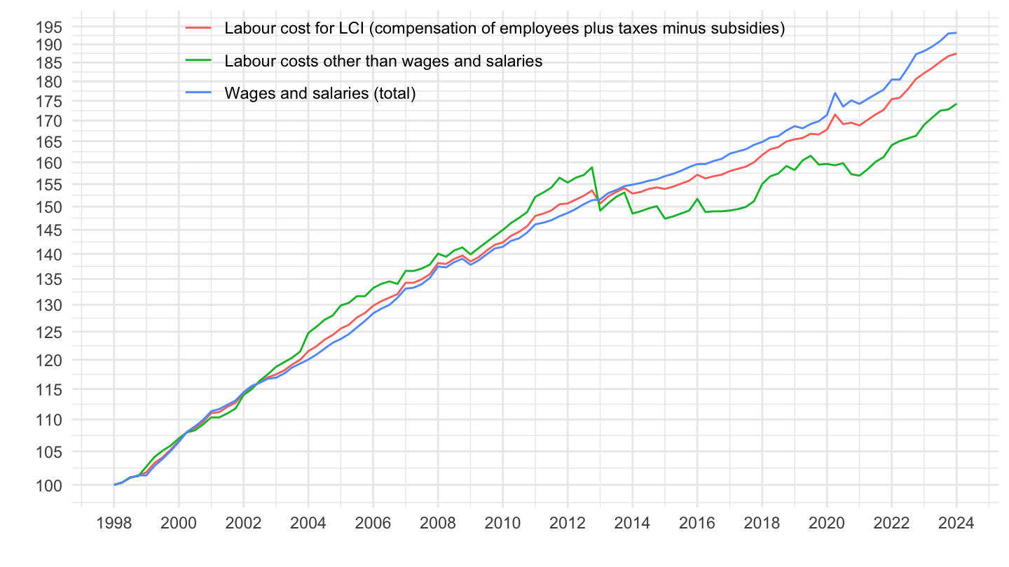
1999-
Code
lc_lci_r2_q %>%
  filter(nace_r2 == "B-N",
         unit == "I20",
         s_adj == "SCA",
         geo %in% c("FR")) %>%
  quarter_to_date %>%
  filter(date >= as.Date("1999-01-01")) %>%


  left_join(colors, by = c("Geo" = "country")) %>%
  group_by(Lcstruct) %>%
  arrange(date) %>%
  mutate(values = 100*values/values[1]) %>%
  ggplot(.) + geom_line(aes(x = date, y = values, color = Lcstruct)) +
  theme_minimal() + xlab("") + ylab("") +
  scale_x_date(breaks = seq(1960, 2100, 2) %>% paste0("-01-01") %>% as.Date,
               labels = date_format("%Y")) +
  scale_y_log10(breaks = seq(50, 200, 5)) +
  theme(legend.position = c(0.45, 0.90),
        legend.title = element_blank())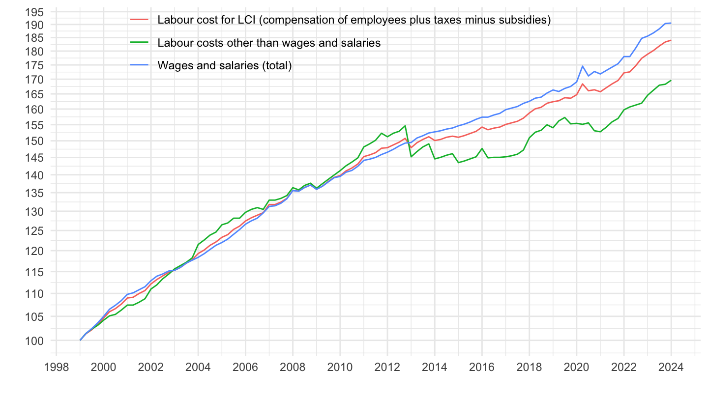
Public
All
Code
lc_lci_r2_q %>%
  filter(nace_r2 == "O-S",
         unit == "I20",
         s_adj == "SCA",
         geo %in% c("FR")) %>%
  quarter_to_date %>%


  left_join(colors, by = c("Geo" = "country")) %>%
  group_by(Lcstruct) %>%
  arrange(date) %>%
  mutate(values = 100*values/values[1]) %>%
  ggplot(.) + geom_line(aes(x = date, y = values, color = Lcstruct)) +
  theme_minimal() + xlab("") + ylab("") +
  scale_x_date(breaks = seq(1960, 2100, 2) %>% paste0("-01-01") %>% as.Date,
               labels = date_format("%Y")) +
  scale_y_log10(breaks = seq(50, 200, 5)) +
  theme(legend.position = c(0.45, 0.90),
        legend.title = element_blank())
2017T2-
Code
lc_lci_r2_q %>%
  filter(nace_r2 == "O-S",
         unit == "I20",
         s_adj == "SCA",
         geo %in% c("FR")) %>%
  quarter_to_date %>%
  filter(date >= as.Date("2017-04-01")) %>%


  left_join(colors, by = c("Geo" = "country")) %>%
  group_by(Lcstruct) %>%
  arrange(date) %>%
  mutate(values = 100*values/values[1]) %>%
  ggplot(.) + geom_line(aes(x = date, y = values, color = Lcstruct)) +
  theme_minimal() + xlab("") + ylab("") +
  scale_x_date(breaks = seq(1960, 2100, 1) %>% paste0("-01-01") %>% as.Date,
               labels = date_format("%Y")) +
  scale_y_log10(breaks = seq(50, 200, 2)) +
  theme(legend.position = c(0.45, 0.90),
        legend.title = element_blank()) +
  geom_text(data = . %>%
              filter(date %in% max(date)),
            aes(x = date, y = values, color = Lcstruct, label = round(values, 1)))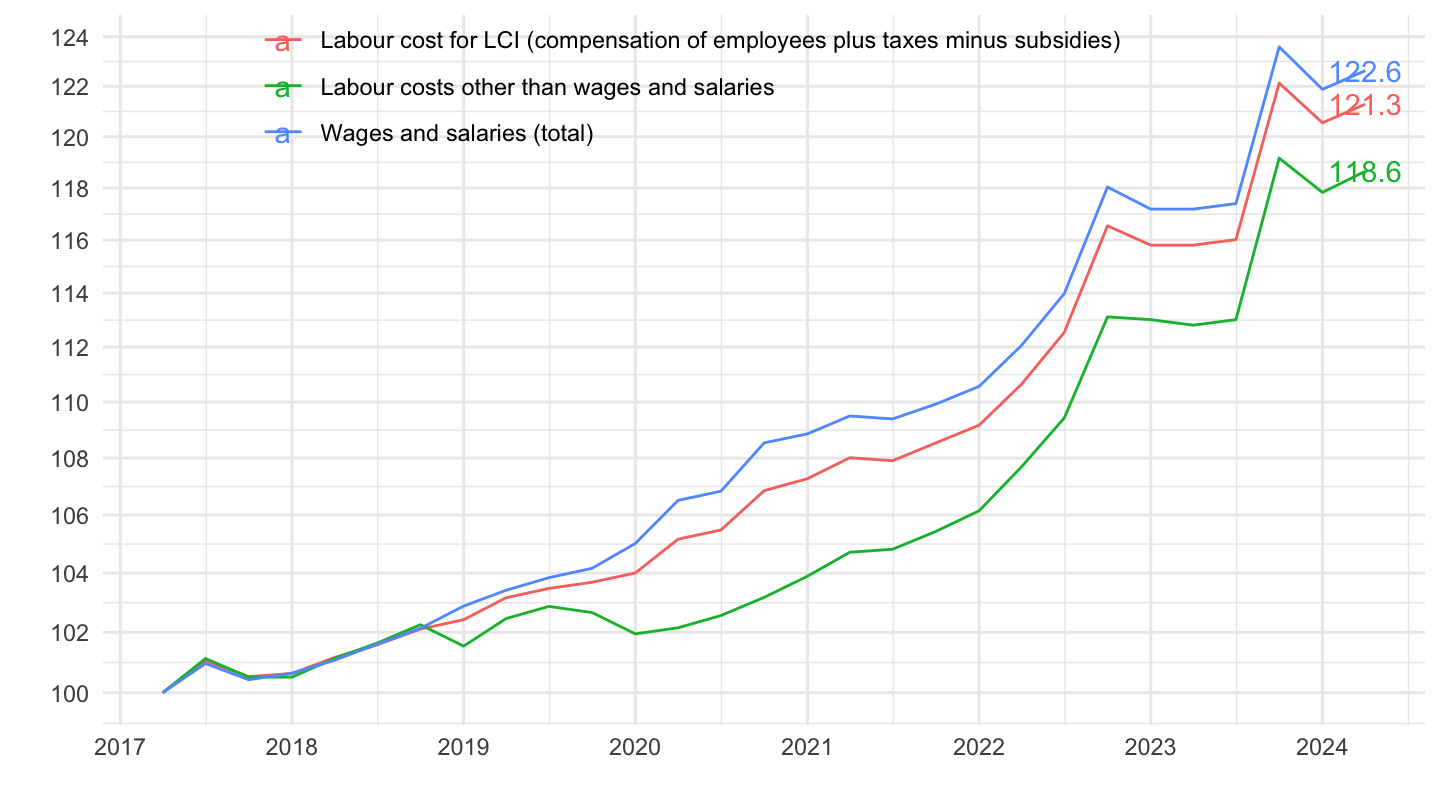
Germany
Code
lc_lci_r2_q %>%
  filter(nace_r2 == "B-S",
         unit == "I20",
         s_adj == "SCA",
         geo %in% c("DE")) %>%
  quarter_to_date %>%


  left_join(colors, by = c("Geo" = "country")) %>%
  group_by(Lcstruct) %>%
  arrange(date) %>%
  mutate(values = 100*values/values[1]) %>%
  ggplot(.) + geom_line(aes(x = date, y = values, color = Lcstruct)) +
  theme_minimal() + xlab("") + ylab("") +
  scale_x_date(breaks = seq(1960, 2100, 2) %>% paste0("-01-01") %>% as.Date,
               labels = date_format("%Y")) +
  scale_y_log10(breaks = seq(60, 200, 5)) +
  theme(legend.position = c(0.45, 0.90),
        legend.title = element_blank())
Italy
Code
lc_lci_r2_q %>%
  filter(nace_r2 == "B-S",
         unit == "I20",
         s_adj == "SCA",
         geo %in% c("IT")) %>%
  quarter_to_date %>%


  left_join(colors, by = c("Geo" = "country")) %>%
  group_by(Lcstruct) %>%
  arrange(date) %>%
  mutate(values = 100*values/values[1]) %>%
  ggplot(.) + geom_line(aes(x = date, y = values, color = Lcstruct)) +
  theme_minimal() + xlab("") + ylab("") +
  scale_x_date(breaks = seq(1960, 2100, 2) %>% paste0("-01-01") %>% as.Date,
               labels = date_format("%Y")) +
  scale_y_continuous(breaks = seq(60, 200, 5)) +
  theme(legend.position = c(0.45, 0.90),
        legend.title = element_blank())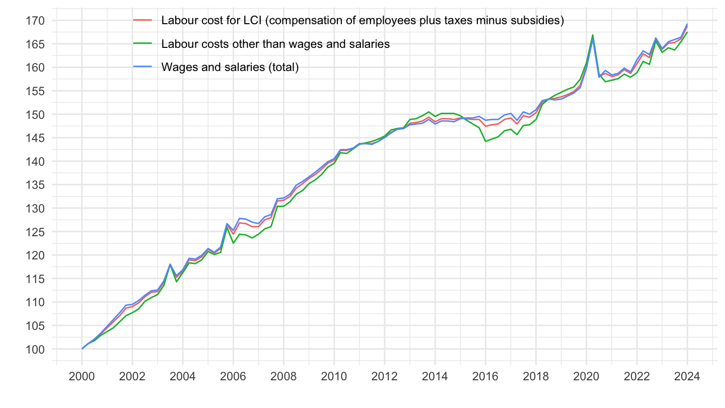
Spain
Code
lc_lci_r2_q %>%
  filter(nace_r2 == "B-S",
         unit == "I20",
         s_adj == "SCA",
         geo %in% c("ES")) %>%
  quarter_to_date %>%


  left_join(colors, by = c("Geo" = "country")) %>%
  group_by(Lcstruct) %>%
  arrange(date) %>%
  mutate(values = 100*values/values[1]) %>%
  ggplot(.) + geom_line(aes(x = date, y = values, color = Lcstruct)) +
  theme_minimal() + xlab("") + ylab("") +
  scale_x_date(breaks = seq(1960, 2100, 2) %>% paste0("-01-01") %>% as.Date,
               labels = date_format("%Y")) +
  scale_y_continuous(breaks = seq(60, 200, 5)) +
  theme(legend.position = c(0.45, 0.90),
        legend.title = element_blank())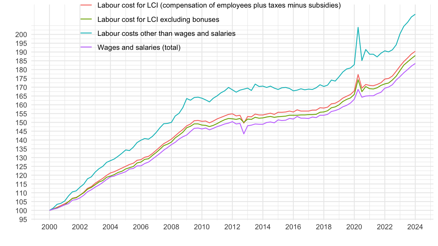
Euro Area
Code
lc_lci_r2_q %>%
  filter(nace_r2 == "B-S",
         unit == "I20",
         s_adj == "SCA",
         geo %in% c("EA")) %>%
  quarter_to_date %>%


  left_join(colors, by = c("Geo" = "country")) %>%
  group_by(Lcstruct) %>%
  arrange(date) %>%
  mutate(values = 100*values/values[1]) %>%
  ggplot(.) + geom_line(aes(x = date, y = values, color = Lcstruct)) +
  theme_minimal() + xlab("") + ylab("") +
  scale_x_date(breaks = seq(1960, 2100, 2) %>% paste0("-01-01") %>% as.Date,
               labels = date_format("%Y")) +
  scale_y_continuous(breaks = seq(60, 200, 5)) +
  theme(legend.position = c(0.45, 0.90),
        legend.title = element_blank())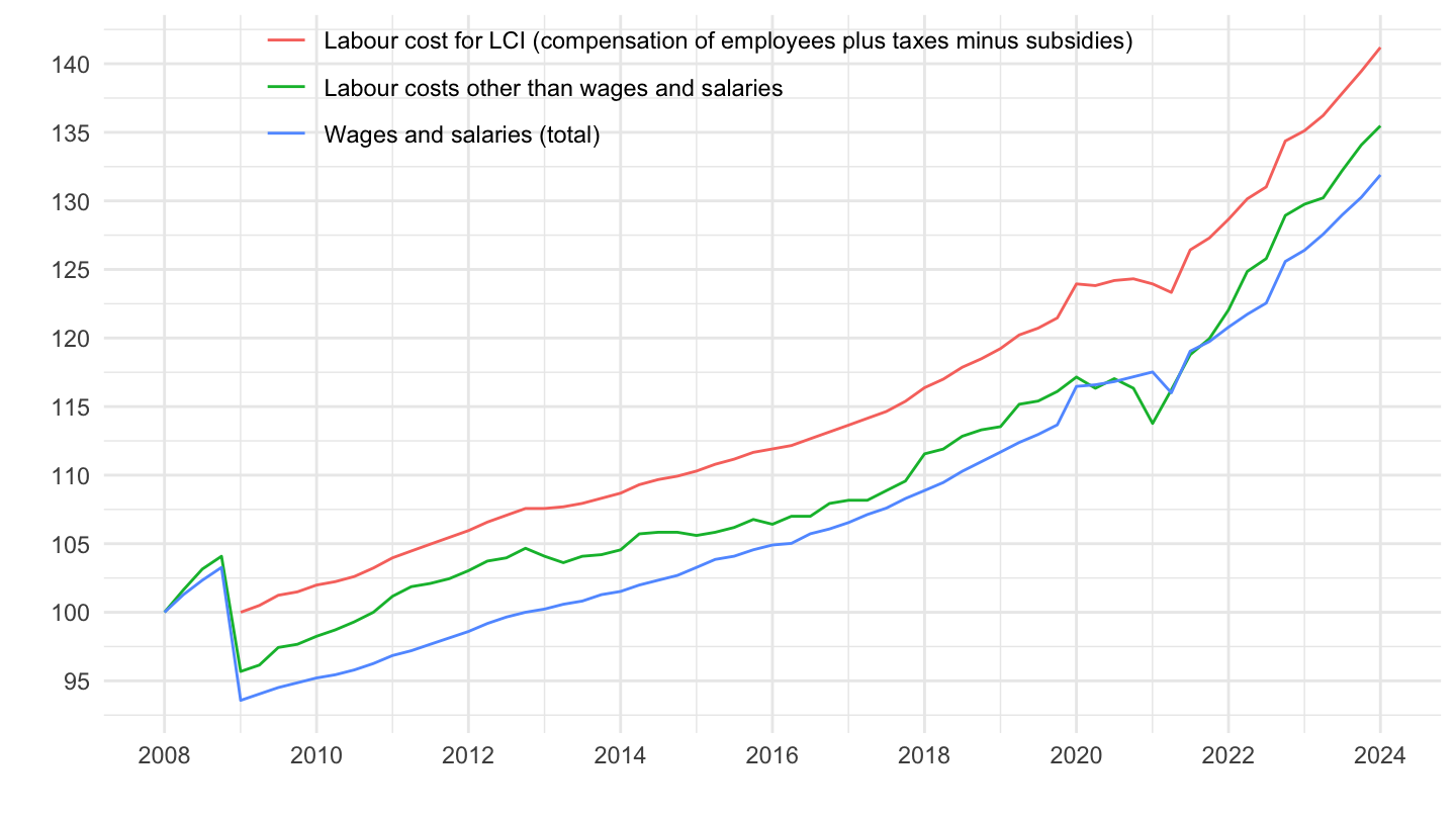
Netherlands
Code
lc_lci_r2_q %>%
  filter(nace_r2 == "B-S",
         unit == "I20",
         s_adj == "SCA",
         geo %in% c("NL")) %>%
  quarter_to_date %>%


  left_join(colors, by = c("Geo" = "country")) %>%
  ggplot(.) + geom_line(aes(x = date, y = values, color = Lcstruct)) +
  theme_minimal() + xlab("") + ylab("") +
  scale_x_date(breaks = seq(1960, 2100, 2) %>% paste0("-01-01") %>% as.Date,
               labels = date_format("%Y")) +
  scale_y_continuous(breaks = seq(60, 200, 5)) +
  theme(legend.position = c(0.45, 0.80),
        legend.title = element_blank())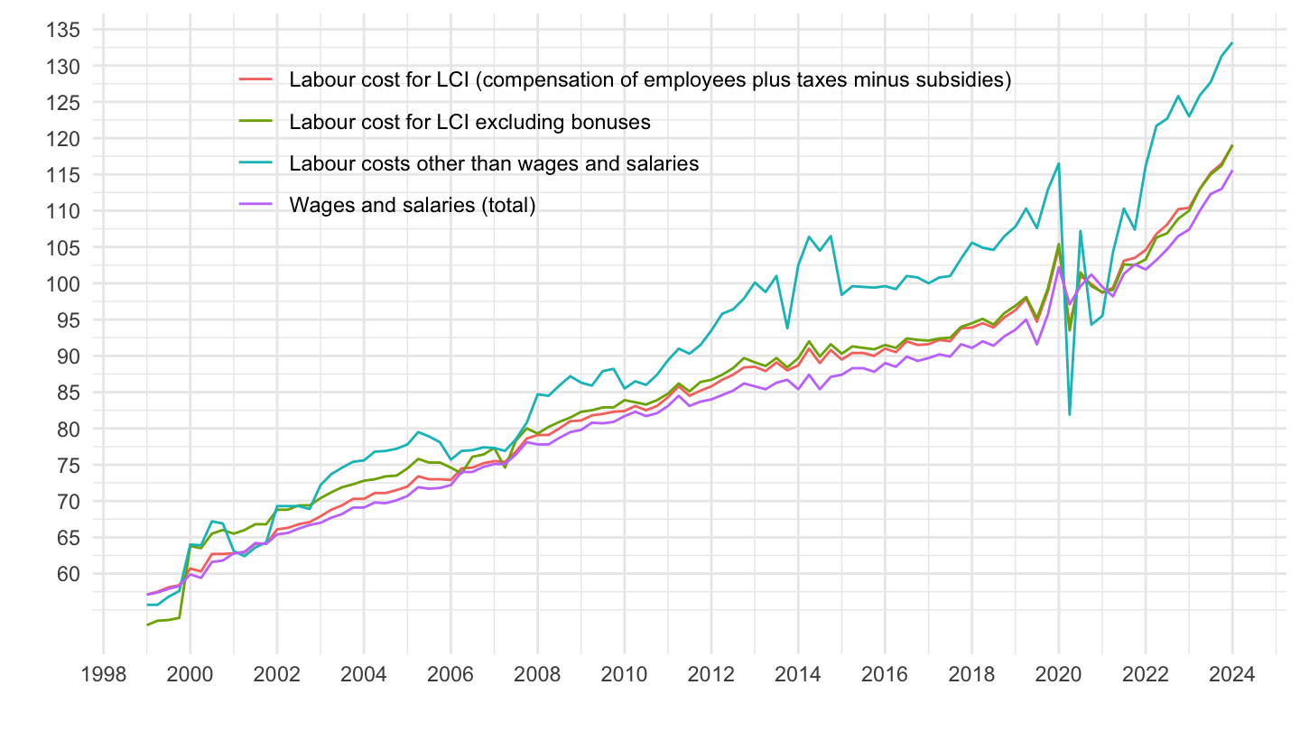
Europe and Eurozone
All
Code
lc_lci_r2_q %>%
  filter(nace_r2 == "B-S",
         unit == "PCH_SM",
         lcstruct == "D11",
         s_adj == "CA",
         geo %in% c("EA19", "EU27_2020")) %>%
  quarter_to_date %>%

  left_join(colors, by = c("Geo" = "country")) %>%
  mutate(values = values/100) %>%
  ggplot(.) + geom_line(aes(x = date, y = values, color = Geo)) +
  theme_minimal() + xlab("") + ylab("") +
  scale_x_date(breaks = seq(1960, 2100, 2) %>% paste0("-01-01") %>% as.Date,
               labels = date_format("%Y")) +
  scale_y_continuous(breaks = 0.01*seq(-20, 20, 1),
                     labels = percent_format(a = 1)) +
  theme(legend.position = c(0.25, 0.90),
        legend.title = element_blank())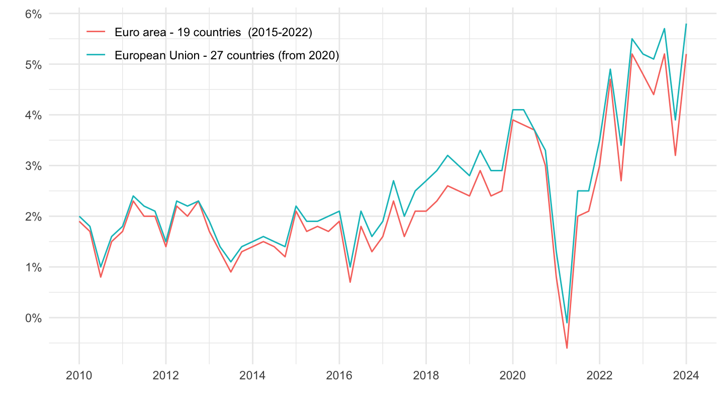
2017-
Code
lc_lci_r2_q %>%
  filter(nace_r2 == "B-S",
         unit == "PCH_SM",
         lcstruct == "D11",
         s_adj == "CA",
         geo %in% c("EA19", "EU27_2020")) %>%
  quarter_to_date %>%
  filter(date >= as.Date("2017-01-01")) %>%

  left_join(colors, by = c("Geo" = "country")) %>%
  mutate(values = values/100) %>%
  ggplot(.) + geom_line(aes(x = date, y = values, color = Geo)) +
  theme_minimal() + xlab("") + ylab("") +
  scale_x_date(breaks = seq(1960, 2100, 1) %>% paste0("-01-01") %>% as.Date,
               labels = date_format("%Y")) +
  scale_y_continuous(breaks = 0.01*seq(-20, 20, 1),
                     labels = percent_format(a = 1)) +
  theme(legend.position = c(0.25, 0.90),
        legend.title = element_blank())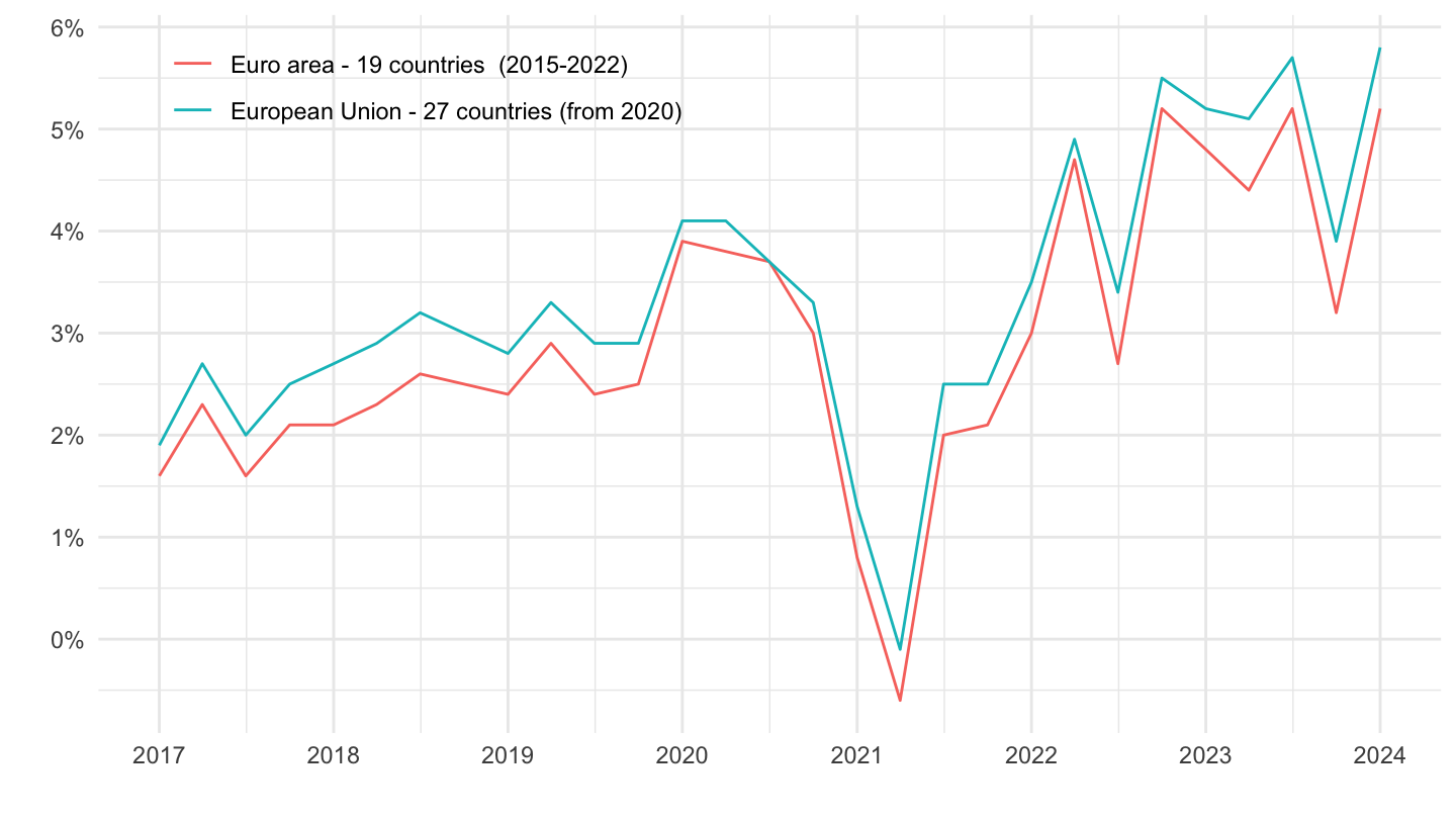
2022Q1-Q2 - Tables
D11 - Wages and salaries (total)
%
Code
lc_lci_r2_q %>%
  filter(nace_r2 == "B-S",
         unit %in% c("PCH_SM", "PCH_PRE"),
         lcstruct == "D11",
         time == max(time),
         s_adj == "CA") %>%


  select_if(~ n_distinct(.) > 1) %>%
  select(-unit) %>%
  spread(Unit, values) %>%
  print_table_conditional()
Indice
Code
lc_lci_r2_q %>%
  filter(nace_r2 == "B-S",
         unit %in% c("PCH_SM", "PCH_PRE"),
         lcstruct == "D11",
         time == max(time),
         s_adj == "CA") %>%


  select_if(~ n_distinct(.) > 1) %>%
  select(-unit) %>%
  spread(Unit, values) %>%
  print_table_conditional()
D12_D4_MD5 - Labour costs other than wages and salaries
Code
lc_lci_r2_q %>%
  filter(nace_r2 == "B-S",
         unit == "PCH_SM",
         lcstruct == "D12_D4_MD5",
         time %in% c("2022Q2","2022Q1"),
         s_adj == "CA") %>%

  select_if(~ n_distinct(.) > 1) %>%
  spread(time, values) %>%
  arrange(`2022Q2`) %>%
  print_table_conditional()
D1_D4_MD5 - Labour cost for LCI (compensation of employees plus taxes minus subsidies)
Code
lc_lci_r2_q %>%
  filter(nace_r2 == "B-S",
         unit == "PCH_SM",
         lcstruct == "D12_D4_MD5",
         time %in% c("2022Q2","2022Q1"),
         s_adj == "CA") %>%

  select_if(~ n_distinct(.) > 1) %>%
  spread(time, values) %>%
  arrange(`2022Q2`) %>%
  print_table_conditional()
D11 - Wages and salaries
France, Germany
Indice
Tous
Code
lc_lci_r2_q %>%
  filter(nace_r2 == "B-N",
         unit == "I20",
         s_adj == "SCA",
         lcstruct == "D11",
         geo %in% c("FR", "DE")) %>%
  quarter_to_date %>%
  #filter(date >= as.Date("1998-01-01")) %>%

  left_join(colors, by = c("Geo" = "country")) %>%
  group_by(geo) %>%
  arrange(date) %>%
  mutate(values = 100*values/values[1]) %>%
  ggplot(.) + geom_line(aes(x = date, y = values, color = color)) +
  theme_minimal() + xlab("") + ylab("") +
  scale_x_date(breaks = c(seq(1998, 2100, 2)) %>% paste0("-01-01") %>% as.Date,
               labels = date_format("%Y")) +
  scale_y_continuous(breaks = seq(90, 200, 5)) +
  scale_color_identity() + add_flags +
  theme(legend.position = c(0.75, 0.90),
        legend.title = element_blank())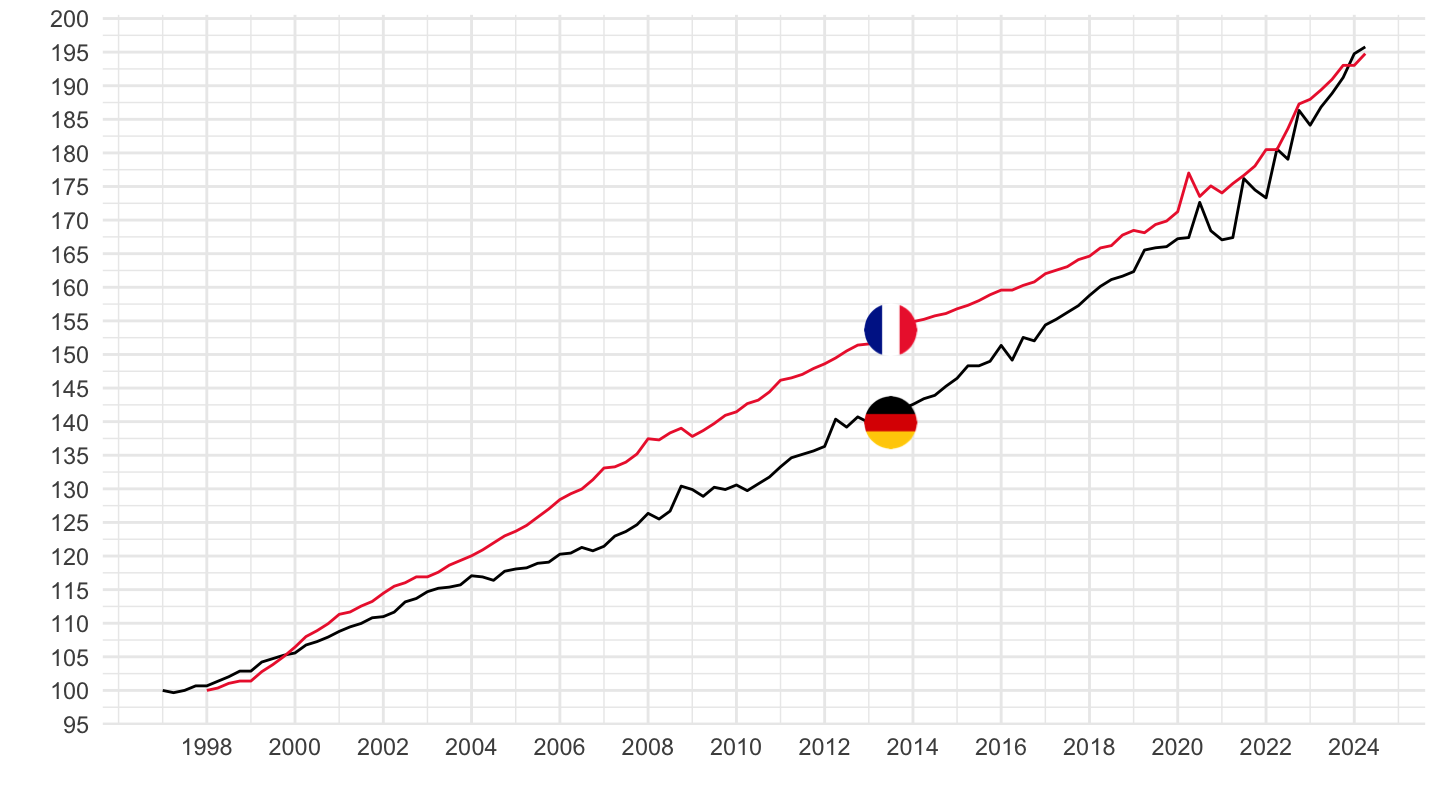
1999-
Code
lc_lci_r2_q %>%
  filter(nace_r2 == "B-N",
         unit == "I20",
         s_adj == "SCA",
         lcstruct == "D11",
         geo %in% c("FR", "DE")) %>%
  quarter_to_date %>%
  filter(date >= as.Date("1999-01-01")) %>%

  left_join(colors, by = c("Geo" = "country")) %>%
  group_by(geo) %>%
  arrange(date) %>%
  mutate(values = 100*values/values[1]) %>%
  ggplot(.) + geom_line(aes(x = date, y = values, color = color)) +
  theme_minimal() + xlab("") + ylab("") +
  scale_x_date(breaks = c(seq(1999, 2100, 5), seq(1997, 2100, 5)) %>% paste0("-01-01") %>% as.Date,
               labels = date_format("%Y")) +
  scale_y_continuous(breaks = seq(90, 200, 5)) +
  scale_color_identity() + add_flags +
  theme(legend.position = c(0.75, 0.90),
        legend.title = element_blank())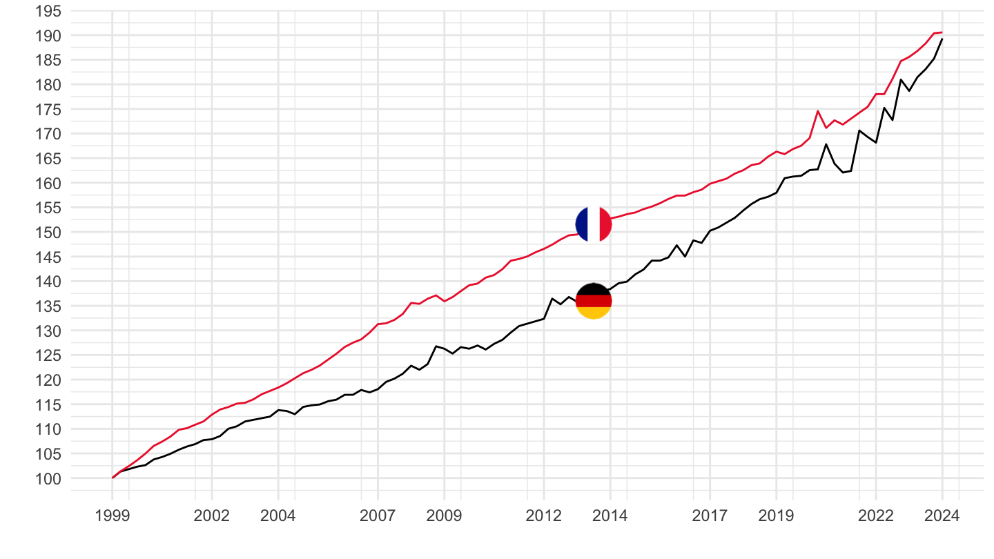
1998-
Code
lc_lci_r2_q %>%
  filter(nace_r2 == "B-N",
         unit == "I20",
         s_adj == "SCA",
         lcstruct == "D11",
         geo %in% c("FR", "DE")) %>%
  quarter_to_date %>%
  filter(date >= as.Date("1998-01-01")) %>%

  left_join(colors, by = c("Geo" = "country")) %>%
  group_by(geo) %>%
  arrange(date) %>%
  mutate(values = 100*values/values[1]) %>%
  ggplot(.) + geom_line(aes(x = date, y = values, color = color)) +
  theme_minimal() + xlab("") + ylab("") +
  scale_x_date(breaks = c(seq(1998, 2100, 2)) %>% paste0("-01-01") %>% as.Date,
               labels = date_format("%Y")) +
  scale_y_continuous(breaks = seq(90, 200, 5)) +
  scale_color_identity() + add_flags +
  theme(legend.position = c(0.75, 0.90),
        legend.title = element_blank())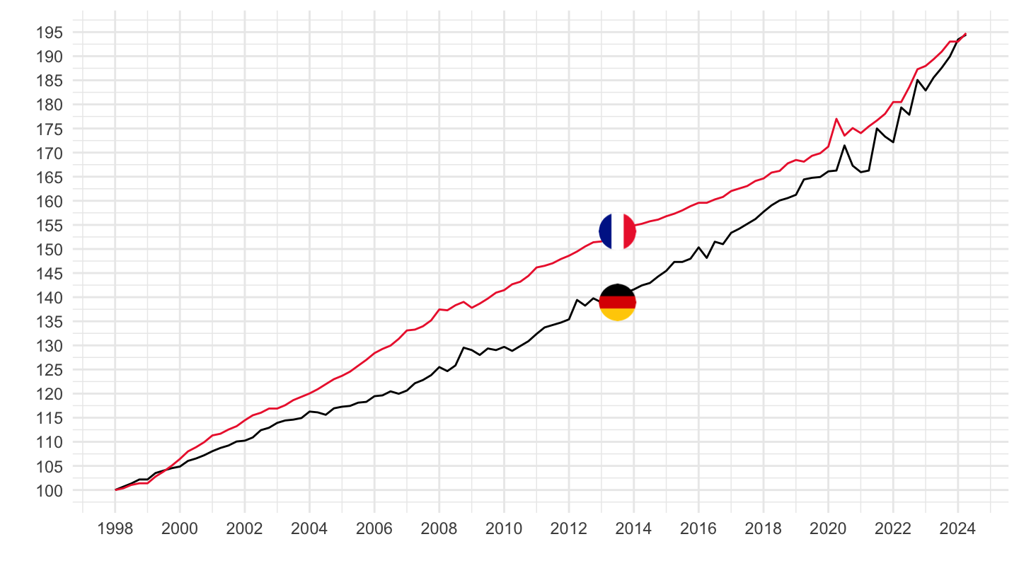
France, Germany, Italy, Spain, Europe
Indice
All
Code
lc_lci_r2_q %>%
  filter(nace_r2 == "B-N",
         unit == "I20",
         s_adj == "SCA",
         lcstruct == "D11",
         geo %in% c("FR", "DE", "ES", "IT", "EA19")) %>%
  quarter_to_date %>%

  mutate(Geo = ifelse(geo == "EA19", "Europe", Geo)) %>%
  left_join(colors, by = c("Geo" = "country")) %>%
  group_by(geo) %>%
  arrange(date) %>%
  mutate(values = 100*values/values[1]) %>%
  ggplot(.) + geom_line(aes(x = date, y = values, color = color)) +
  theme_minimal() + xlab("") + ylab("") +
  scale_x_date(breaks = seq(1960, 2100, 2) %>% paste0("-01-01") %>% as.Date,
               labels = date_format("%Y")) +
  scale_y_continuous(breaks = seq(90, 200, 5)) +
  scale_color_identity() + add_flags +
  theme(legend.position = c(0.75, 0.90),
        legend.title = element_blank())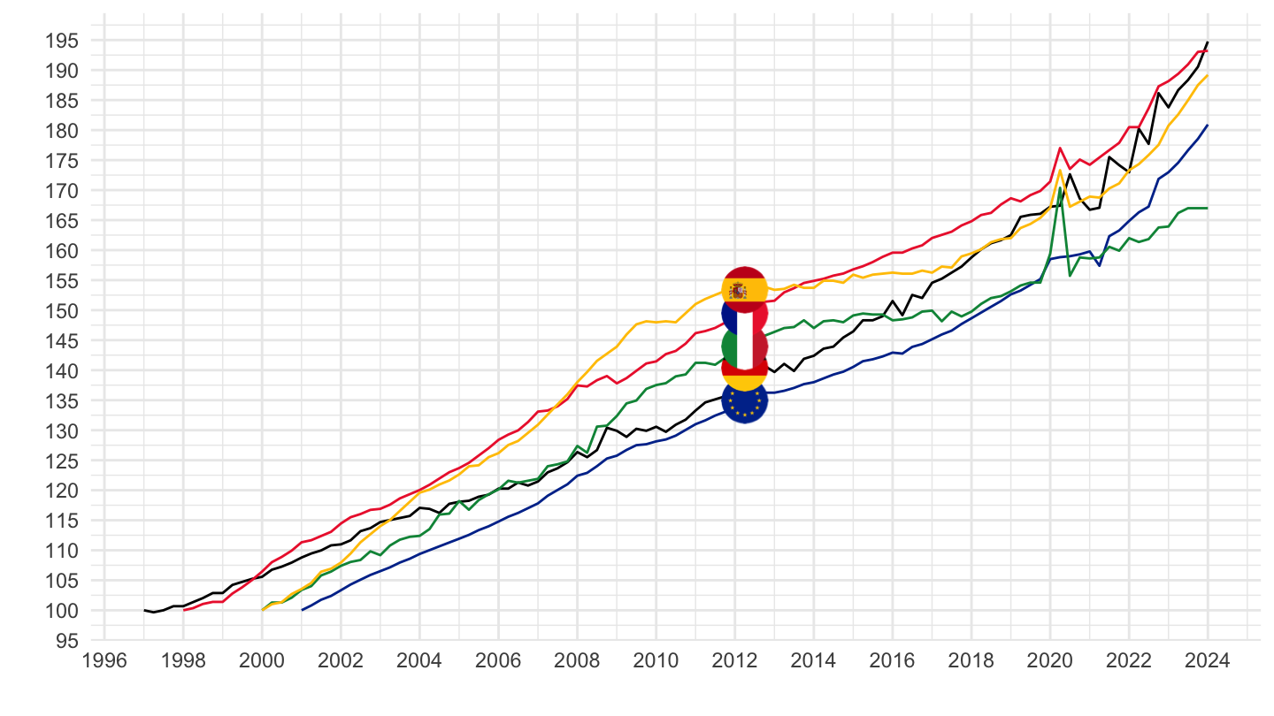
2001-
Code
lc_lci_r2_q %>%
  filter(nace_r2 == "B-N",
         unit == "I20",
         s_adj == "SCA",
         lcstruct == "D11",
         geo %in% c("FR", "DE", "ES", "IT", "EA19")) %>%
  quarter_to_date %>%
  filter(date >= as.Date("2001-01-01")) %>%

  mutate(Geo = ifelse(geo == "EA19", "Europe", Geo)) %>%
  left_join(colors, by = c("Geo" = "country")) %>%
  group_by(geo) %>%
  arrange(date) %>%
  mutate(values = 100*values/values[1]) %>%
  ggplot(.) + geom_line(aes(x = date, y = values, color = color)) +
  theme_minimal() + xlab("") + ylab("") +
  scale_x_date(breaks = seq(1960, 2100, 2) %>% paste0("-01-01") %>% as.Date,
               labels = date_format("%Y")) +
  scale_y_continuous(breaks = seq(90, 200, 5)) +
  scale_color_identity() + add_flags +
  theme(legend.position = c(0.75, 0.90),
        legend.title = element_blank())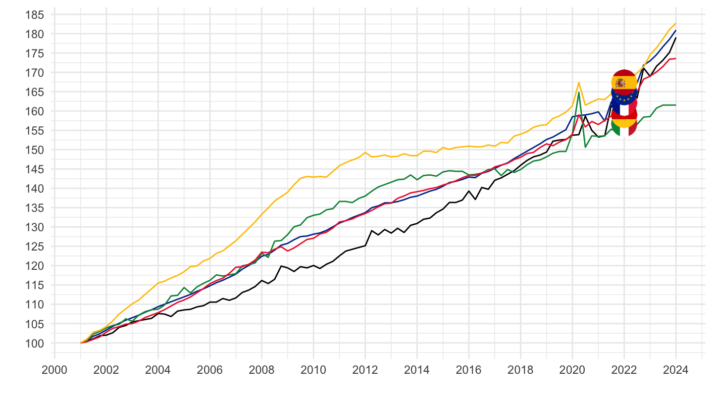
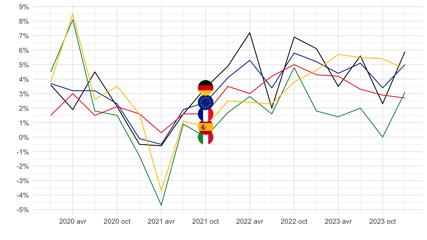
2017T2-
B-N
Code
lc_lci_r2_q %>%
  filter(nace_r2 == "B-N",
         unit == "I20",
         s_adj == "SCA",
         lcstruct == "D11",
         geo %in% c("FR", "DE", "ES", "IT", "EA20")) %>%
  quarter_to_date %>%
  filter(date >= as.Date("2017-04-01")) %>%

  mutate(Geo = ifelse(geo == "EA20", "Europe", Geo)) %>%
  left_join(colors, by = c("Geo" = "country")) %>%
  group_by(geo) %>%
  arrange(date) %>%
  mutate(values = 100*values/values[1]) %>%
  ggplot(.) + geom_line(aes(x = date, y = values, color = color)) +
  theme_minimal() + xlab("") + ylab("") +
  scale_x_date(breaks = seq(1960, 2100, 1) %>% paste0("-01-01") %>% as.Date,
               labels = date_format("%Y")) +
  scale_y_continuous(breaks = seq(90, 200, 5)) +
  scale_color_identity() + add_flags +
  theme(legend.position = c(0.75, 0.90),
        legend.title = element_blank())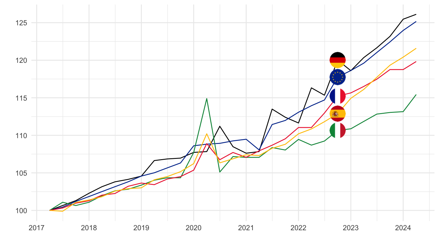
B-S
Code
lc_lci_r2_q %>%
  filter(nace_r2 == "B-S",
         unit == "I20",
         s_adj == "SCA",
         lcstruct == "D11",
         geo %in% c("FR", "DE", "ES", "IT", "EA20")) %>%
  quarter_to_date %>%
  filter(date >= as.Date("2017-04-01")) %>%

  mutate(Geo = ifelse(geo == "EA20", "Europe", Geo)) %>%
  left_join(colors, by = c("Geo" = "country")) %>%
  group_by(geo) %>%
  arrange(date) %>%
  mutate(values = 100*values/values[1]) %>%
  ggplot(.) + geom_line(aes(x = date, y = values, color = color)) +
  theme_minimal() + xlab("") + ylab("") +
  scale_x_date(breaks = seq(1960, 2100, 1) %>% paste0("-01-01") %>% as.Date,
               labels = date_format("%Y")) +
  scale_y_continuous(breaks = seq(90, 200, 5)) +
  scale_color_identity() + add_flags +
  theme(legend.position = c(0.75, 0.90),
        legend.title = element_blank())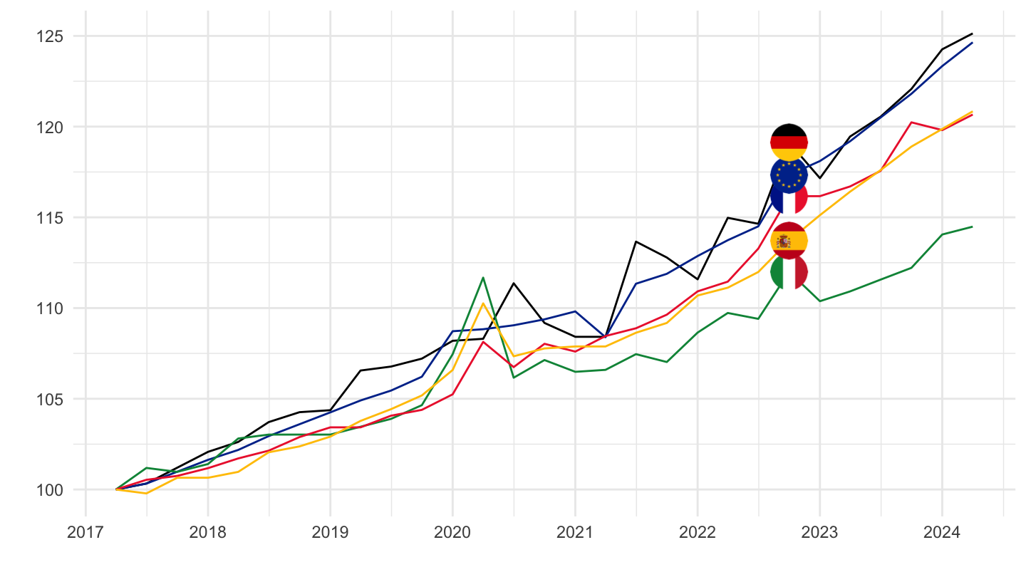
Change
All
Code
lc_lci_r2_q %>%
  filter(nace_r2 == "B-S",
         unit == "PCH_SM",
         lcstruct == "D11",
         s_adj == "CA",
         geo %in% c("FR", "DE", "ES", "IT", "EA19")) %>%
  quarter_to_date %>%

  mutate(values = values/100,
         Geo = ifelse(geo == "EA19", "Europe", Geo)) %>%
  left_join(colors, by = c("Geo" = "country")) %>%
  ggplot(.) + geom_line(aes(x = date, y = values, color = color)) +
  theme_minimal() + xlab("") + ylab("") +
  scale_x_date(breaks = seq(1960, 2100, 2) %>% paste0("-01-01") %>% as.Date,
               labels = date_format("%Y")) +
  scale_y_continuous(breaks = 0.01*seq(-20, 20, 1),
                     labels = percent_format(a = 1)) +
  scale_color_identity() + add_flags +
  theme(legend.position = c(0.75, 0.90),
        legend.title = element_blank())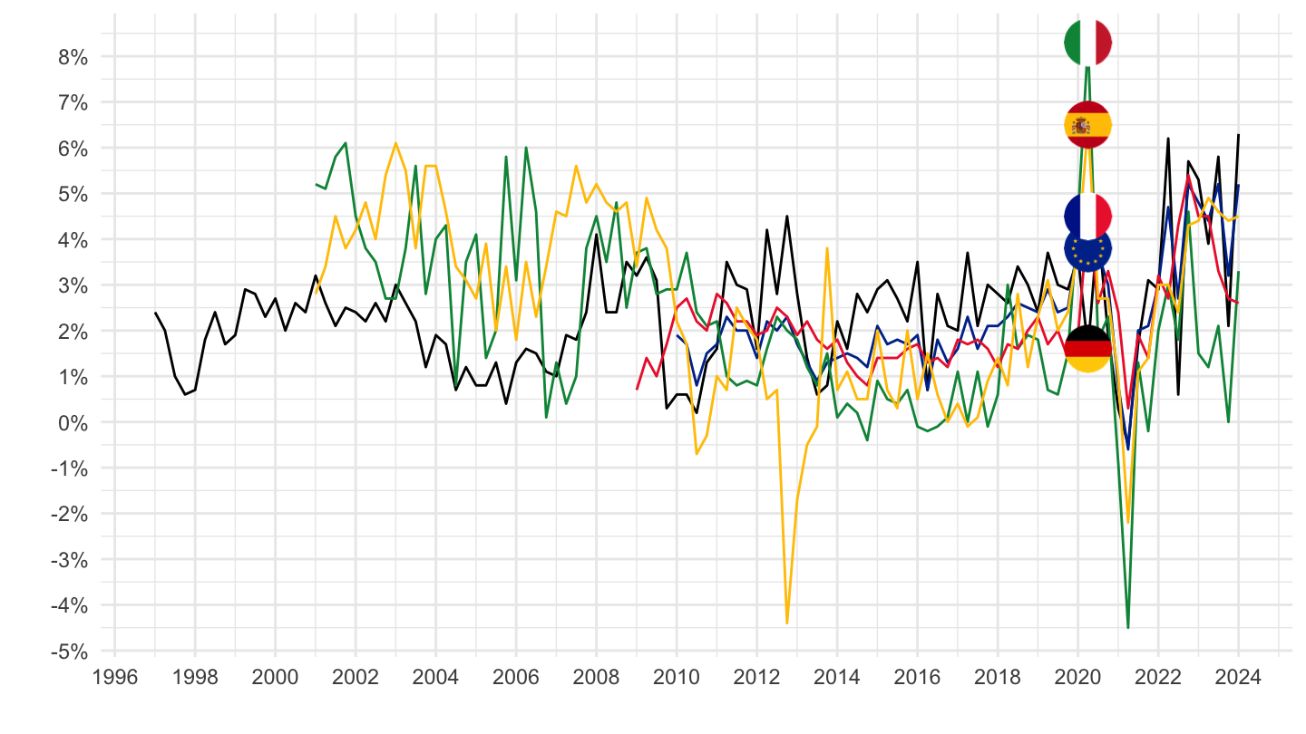
2017-
Code
lc_lci_r2_q %>%
  filter(nace_r2 == "B-S",
         unit == "PCH_SM",
         lcstruct == "D11",
         s_adj == "CA",
         geo %in% c("FR", "DE", "ES", "IT", "EA19")) %>%
  quarter_to_date %>%
  filter(date >= as.Date("2017-01-01")) %>%

  mutate(values = values/100,
         Geo = ifelse(geo == "EA19", "Europe", Geo)) %>%
  left_join(colors, by = c("Geo" = "country")) %>%
  ggplot(.) + geom_line(aes(x = date, y = values, color = color)) +
  theme_minimal() + xlab("") + ylab("") +
  scale_x_date(breaks = seq(1960, 2100, 1) %>% paste0("-01-01") %>% as.Date,
               labels = date_format("%Y")) +
  scale_y_continuous(breaks = 0.01*seq(-20, 20, 1),
                     labels = percent_format(a = 1)) +
  scale_color_identity() + add_flags +
  theme(legend.position = c(0.75, 0.90),
        legend.title = element_blank())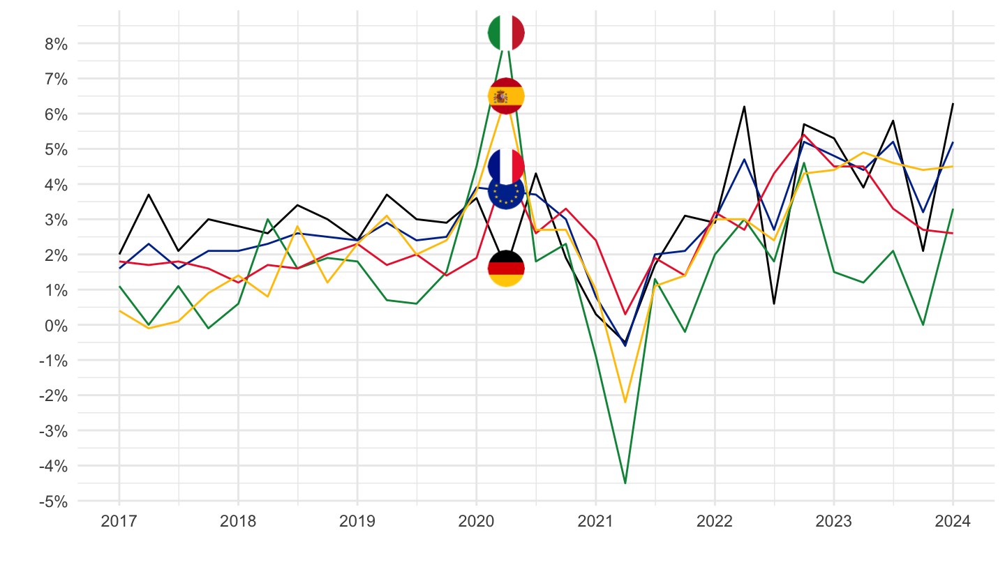
2020-
Code
lc_lci_r2_q %>%
  filter(nace_r2 == "B-S",
         unit == "PCH_SM",
         lcstruct == "D11",
         s_adj == "CA",
         geo %in% c("FR", "DE", "ES", "IT", "EA19")) %>%
  quarter_to_date %>%
  filter(date >= as.Date("2020-01-01")) %>%

  mutate(values = values/100,
         Geo = ifelse(geo == "EA19", "Europe", Geo)) %>%
  left_join(colors, by = c("Geo" = "country")) %>%
  ggplot(.) + geom_line(aes(x = date, y = values, color = color)) +
  theme_minimal() + xlab("") + ylab("") +
  scale_x_date(breaks = "6 months",
               labels = date_format("%Y %b")) +
  scale_y_continuous(breaks = 0.01*seq(-20, 20, 1),
                     labels = percent_format(a = 1)) +
  scale_color_identity() + add_flags +
  theme(legend.position = c(0.75, 0.90),
        legend.title = element_blank())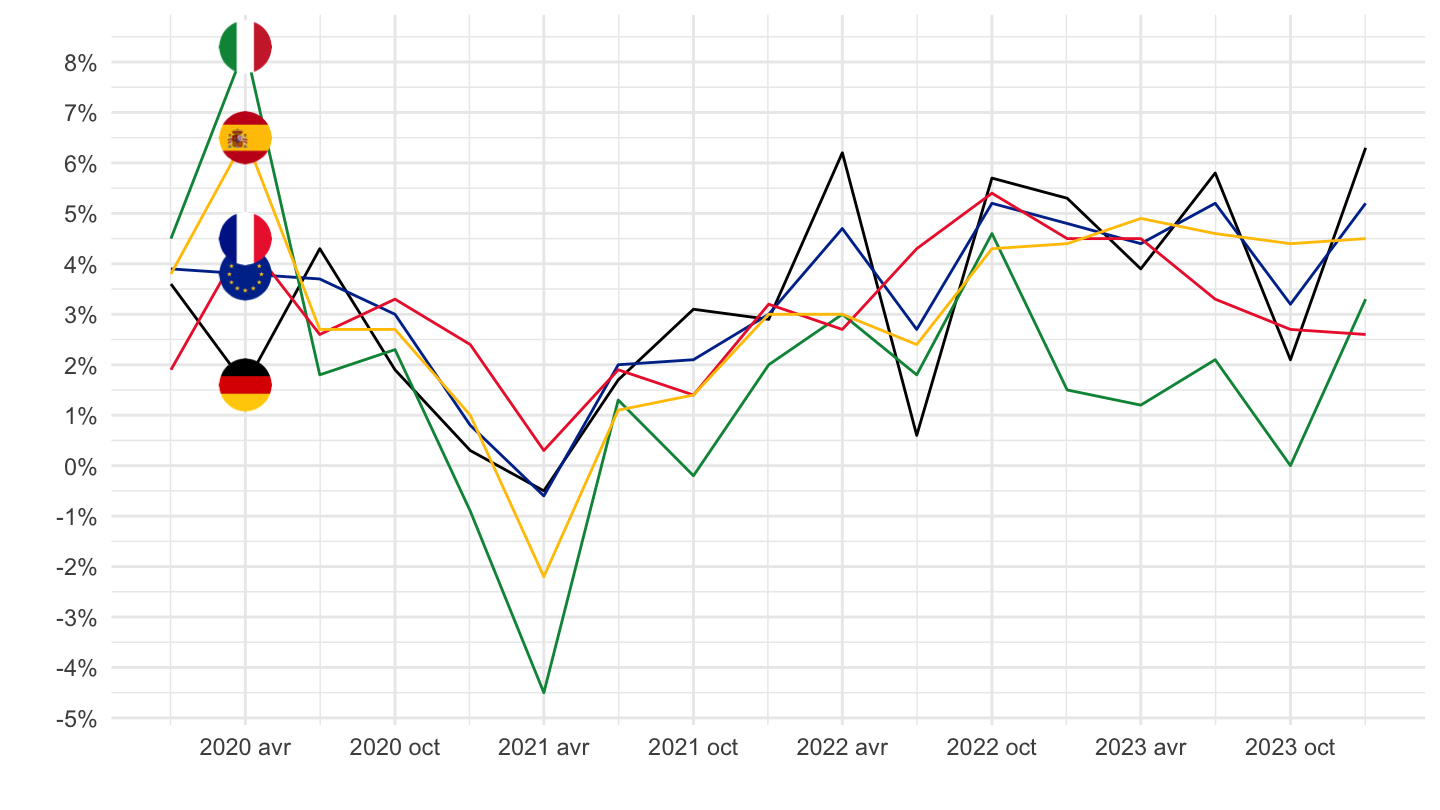
3 years
Code
lc_lci_r2_q %>%
  filter(nace_r2 == "B-S",
         unit == "PCH_SM",
         lcstruct == "D11",
         s_adj == "CA",
         geo %in% c("FR", "DE", "ES", "IT", "EA19")) %>%
  quarter_to_date %>%
  filter(date >= Sys.Date() - years(3)) %>%

  mutate(values = values/100,
         Geo = ifelse(geo == "EA19", "Europe", Geo)) %>%
  left_join(colors, by = c("Geo" = "country")) %>%
  ggplot(.) + geom_line(aes(x = date, y = values, color = color)) +
  theme_minimal() + xlab("") + ylab("") +
  scale_x_date(breaks = "3 months",
               labels = date_format("%Y %b")) +
  scale_y_continuous(breaks = 0.01*seq(-20, 20, 1),
                     labels = percent_format(a = 1)) +
  scale_color_identity() + add_flags +
  theme(legend.position = c(0.75, 0.90),
        legend.title = element_blank())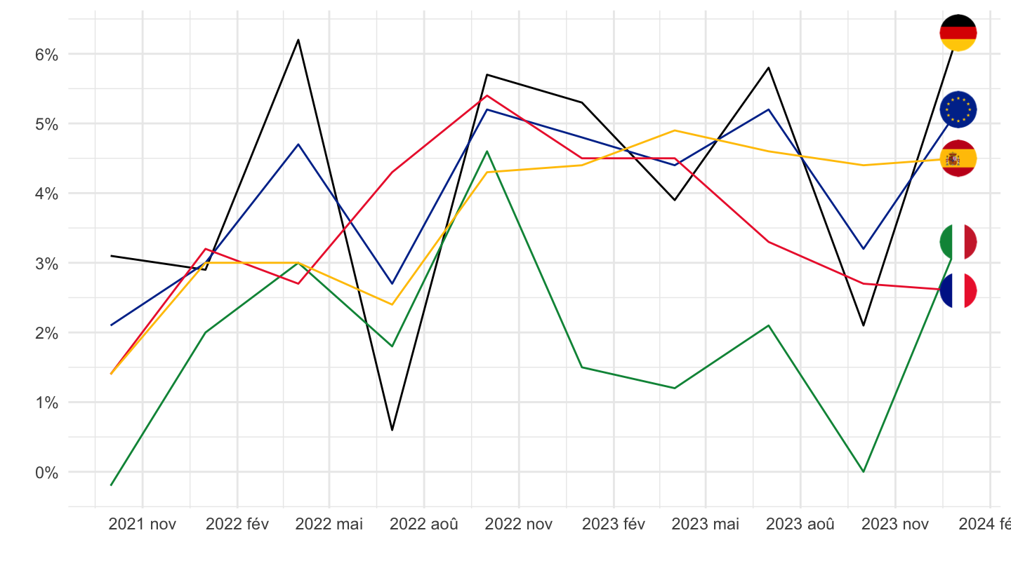
2 years
Code
lc_lci_r2_q %>%
  filter(nace_r2 == "B-S",
         unit == "PCH_SM",
         lcstruct == "D11",
         s_adj == "CA",
         geo %in% c("FR", "DE", "ES", "IT", "EA19")) %>%
  quarter_to_date %>%
  filter(date >= Sys.Date() - years(2)) %>%

  mutate(values = values/100,
         Geo = ifelse(geo == "EA19", "Europe", Geo)) %>%
  left_join(colors, by = c("Geo" = "country")) %>%
  ggplot(.) + geom_line(aes(x = date, y = values, color = color)) +
  theme_minimal() + xlab("") + ylab("") +
  scale_x_date(breaks = "3 months",
               labels = date_format("%Y %b")) +
  scale_y_continuous(breaks = 0.01*seq(-20, 20, 1),
                     labels = percent_format(a = 1)) +
  scale_color_identity() + add_flags +
  theme(legend.position = c(0.75, 0.90),
        legend.title = element_blank())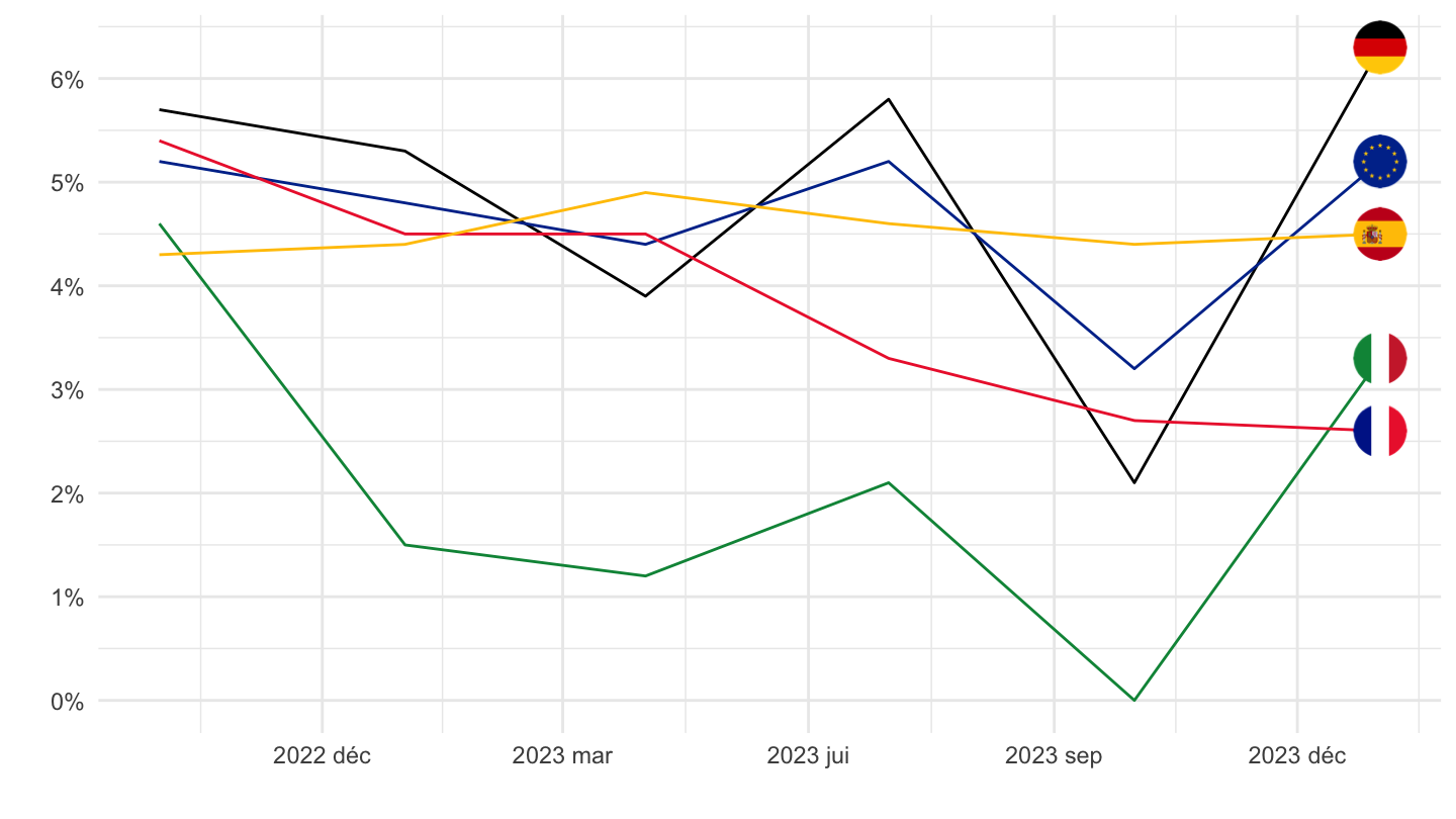
Netherlands, Portugal, Hungary, Italy
All
Code
lc_lci_r2_q %>%
  filter(nace_r2 == "B-S",
         unit == "PCH_SM",
         lcstruct == "D11",
         s_adj == "CA",
         geo %in% c("NL", "PT", "HU", "IT")) %>%
  quarter_to_date %>%

  left_join(colors, by = c("Geo" = "country")) %>%
  mutate(values = values/100) %>%
  ggplot(.) + geom_line(aes(x = date, y = values, color = color)) +
  theme_minimal() + xlab("") + ylab("") +
  scale_x_date(breaks = seq(1960, 2100, 2) %>% paste0("-01-01") %>% as.Date,
               labels = date_format("%Y")) +
  scale_y_continuous(breaks = 0.01*seq(-20, 20, 1),
                     labels = percent_format(a = 1)) +
  scale_color_identity() + add_flags +
  theme(legend.position = c(0.75, 0.90),
        legend.title = element_blank())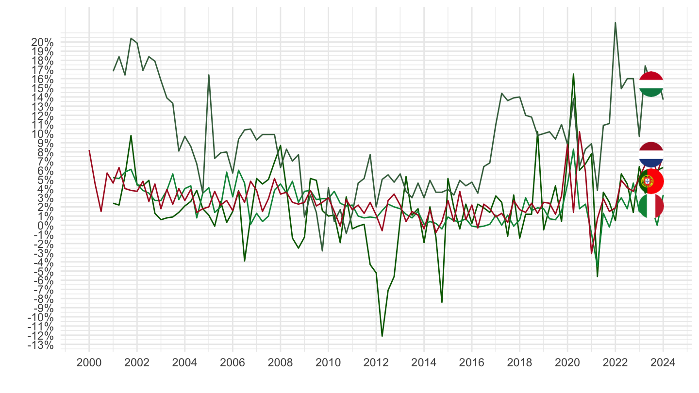
2017-
Code
lc_lci_r2_q %>%
  filter(nace_r2 == "B-S",
         unit == "PCH_SM",
         lcstruct == "D11",
         s_adj == "CA",
         geo %in% c("NL", "PT", "HU", "IT")) %>%
  quarter_to_date %>%
  filter(date >= as.Date("2017-01-01")) %>%

  left_join(colors, by = c("Geo" = "country")) %>%
  mutate(values = values/100) %>%
  ggplot(.) + geom_line(aes(x = date, y = values, color = color)) +
  theme_minimal() + xlab("") + ylab("") +
  scale_x_date(breaks = seq(1960, 2100, 1) %>% paste0("-01-01") %>% as.Date,
               labels = date_format("%Y")) +
  scale_y_continuous(breaks = 0.01*seq(-20, 20, 1),
                     labels = percent_format(a = 1)) +
  scale_color_identity() + add_flags +
  theme(legend.position = c(0.75, 0.90),
        legend.title = element_blank())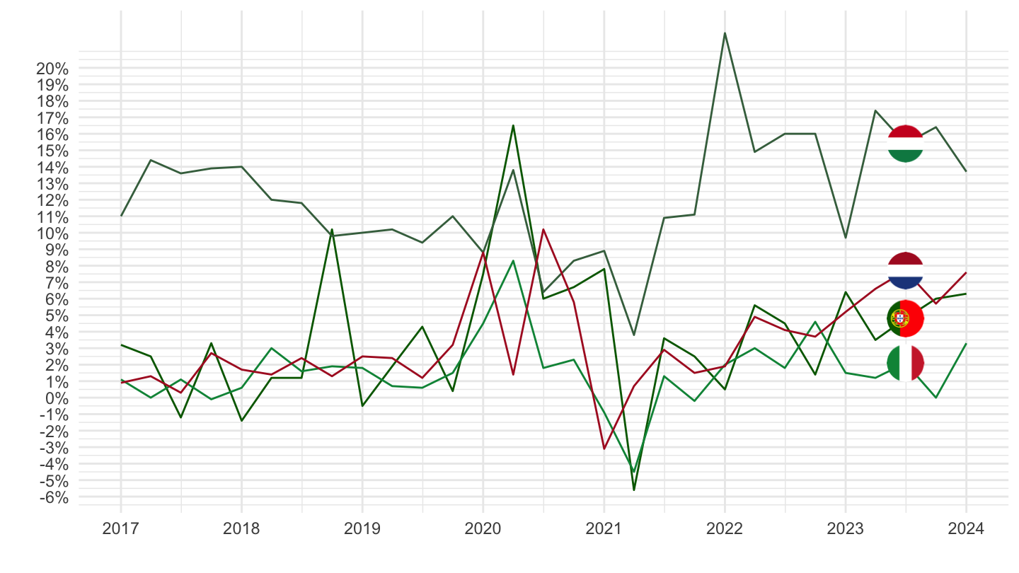
D12_D4_MD5 - Labour costs other than wages and salaries
France, Germany, Italy, Spain, Europe
All
Code
lc_lci_r2_q %>%
  filter(nace_r2 == "B-S",
         unit == "PCH_SM",
         lcstruct == "D12_D4_MD5",
         s_adj == "CA",
         geo %in% c("FR", "DE", "ES", "IT", "EA19")) %>%
  quarter_to_date %>%

  mutate(values = values/100,
         Geo = ifelse(geo == "EA19", "Europe", Geo)) %>%
  left_join(colors, by = c("Geo" = "country")) %>%
  ggplot(.) + geom_line(aes(x = date, y = values, color = color)) +
  theme_minimal() + xlab("") + ylab("") +
  scale_x_date(breaks = seq(1960, 2100, 2) %>% paste0("-01-01") %>% as.Date,
               labels = date_format("%Y")) +
  scale_y_continuous(breaks = 0.01*seq(-20, 20, 1),
                     labels = percent_format(a = 1)) +
  scale_color_identity() + add_flags +
  theme(legend.position = c(0.75, 0.90),
        legend.title = element_blank())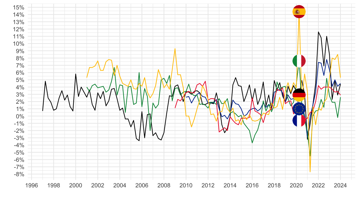
2017-
Code
lc_lci_r2_q %>%
  filter(nace_r2 == "B-S",
         unit == "PCH_SM",
         lcstruct == "D12_D4_MD5",
         s_adj == "CA",
         geo %in% c("FR", "DE", "ES", "IT", "EA19")) %>%
  quarter_to_date %>%
  filter(date >= as.Date("2017-01-01")) %>%

  mutate(values = values/100,
         Geo = ifelse(geo == "EA19", "Europe", Geo)) %>%
  left_join(colors, by = c("Geo" = "country")) %>%
  ggplot(.) + geom_line(aes(x = date, y = values, color = color)) +
  theme_minimal() + xlab("") + ylab("") +
  scale_x_date(breaks = seq(1960, 2100, 1) %>% paste0("-01-01") %>% as.Date,
               labels = date_format("%Y")) +
  scale_y_continuous(breaks = 0.01*seq(-20, 20, 1),
                     labels = percent_format(a = 1)) +
  scale_color_identity() + add_flags +
  theme(legend.position = c(0.75, 0.90),
        legend.title = element_blank())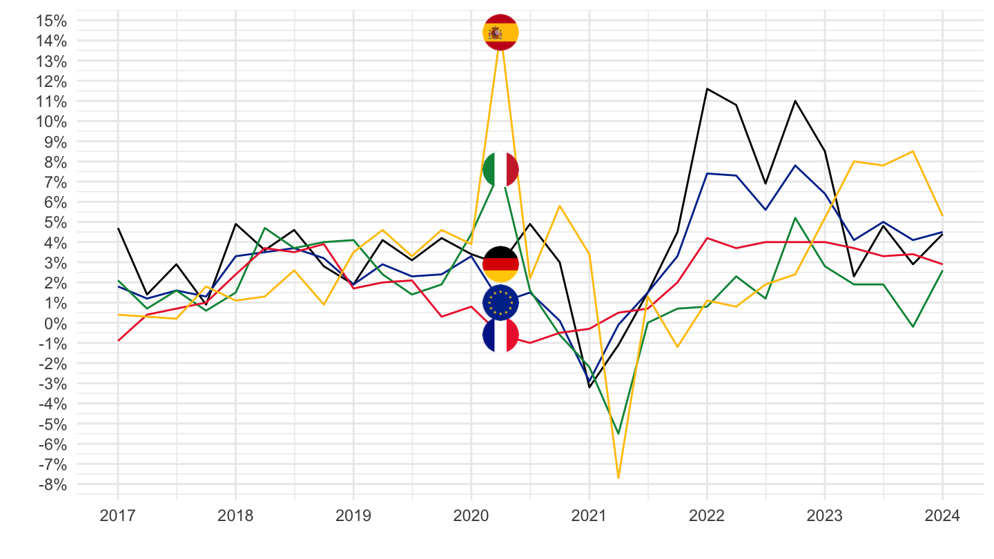
2020-
Code
lc_lci_r2_q %>%
  filter(nace_r2 == "B-S",
         unit == "PCH_SM",
         lcstruct == "D12_D4_MD5",
         s_adj == "CA",
         geo %in% c("FR", "DE", "ES", "IT", "EA19")) %>%
  quarter_to_date %>%
  filter(date >= as.Date("2020-01-01")) %>%

  mutate(values = values/100,
         Geo = ifelse(geo == "EA19", "Europe", Geo)) %>%
  left_join(colors, by = c("Geo" = "country")) %>%
  ggplot(.) + geom_line(aes(x = date, y = values, color = color)) +
  theme_minimal() + xlab("") + ylab("") +
  scale_x_date(breaks = "6 months",
               labels = date_format("%Y %b")) +
  scale_y_continuous(breaks = 0.01*seq(-20, 20, 1),
                     labels = percent_format(a = 1)) +
  scale_color_identity() + add_flags +
  theme(legend.position = c(0.75, 0.90),
        legend.title = element_blank())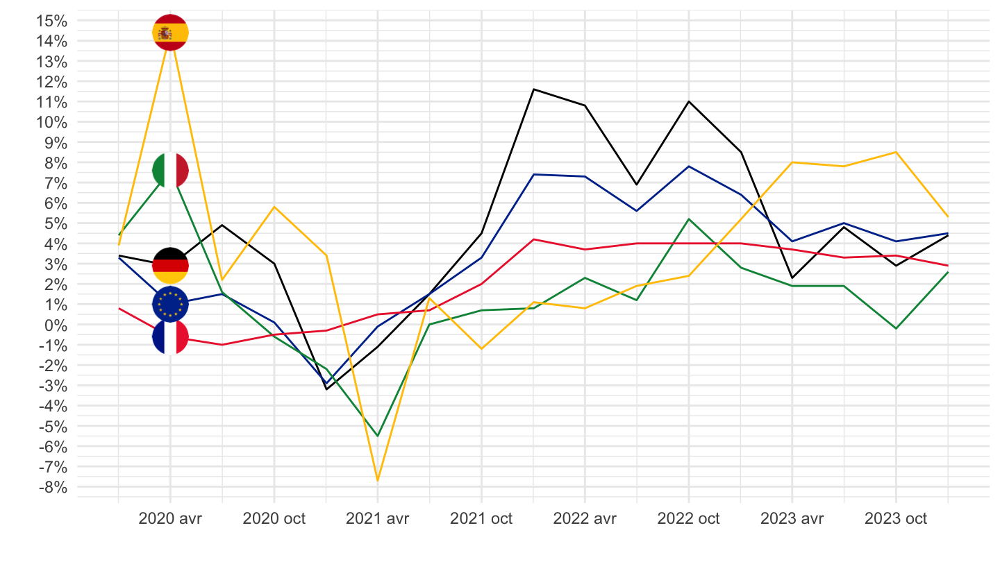
3 years
Code
lc_lci_r2_q %>%
  filter(nace_r2 == "B-S",
         unit == "PCH_SM",
         lcstruct == "D12_D4_MD5",
         s_adj == "CA",
         geo %in% c("FR", "DE", "ES", "IT", "EA19")) %>%
  quarter_to_date %>%
  filter(date >= Sys.Date() - years(3)) %>%

  mutate(values = values/100,
         Geo = ifelse(geo == "EA19", "Europe", Geo)) %>%
  left_join(colors, by = c("Geo" = "country")) %>%
  ggplot(.) + geom_line(aes(x = date, y = values, color = color)) +
  theme_minimal() + xlab("") + ylab("") +
  scale_x_date(breaks = "3 months",
               labels = date_format("%Y %b")) +
  scale_y_continuous(breaks = 0.01*seq(-20, 20, 1),
                     labels = percent_format(a = 1)) +
  scale_color_identity() + add_flags +
  theme(legend.position = c(0.75, 0.90),
        legend.title = element_blank())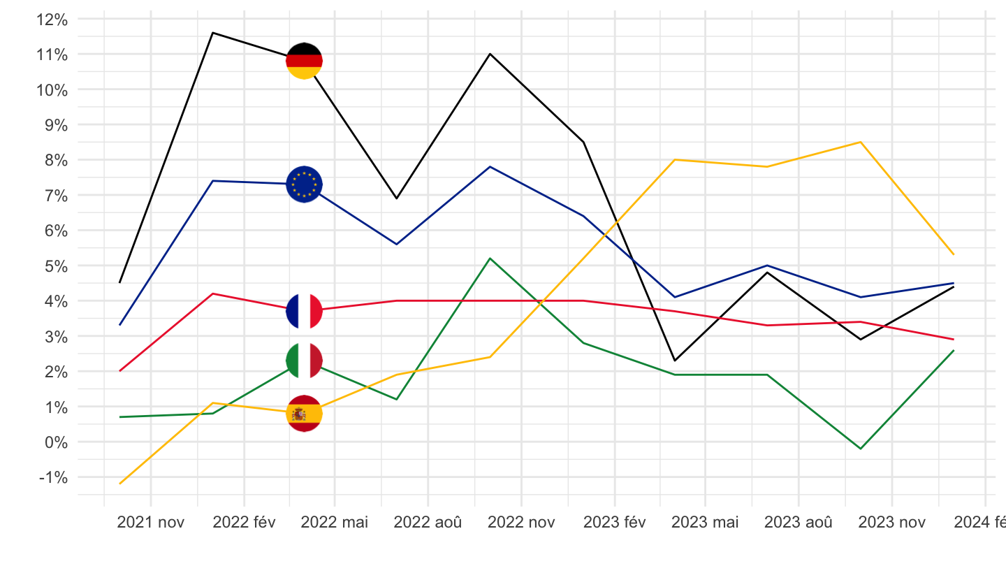
2 years
Code
lc_lci_r2_q %>%
  filter(nace_r2 == "B-S",
         unit == "PCH_SM",
         lcstruct == "D12_D4_MD5",
         s_adj == "CA",
         geo %in% c("FR", "DE", "ES", "IT", "EA19")) %>%
  quarter_to_date %>%
  filter(date >= Sys.Date() - years(2)) %>%

  mutate(values = values/100,
         Geo = ifelse(geo == "EA19", "Europe", Geo)) %>%
  left_join(colors, by = c("Geo" = "country")) %>%
  ggplot(.) + geom_line(aes(x = date, y = values, color = color)) +
  theme_minimal() + xlab("") + ylab("") +
  scale_x_date(breaks = "3 months",
               labels = date_format("%Y %b")) +
  scale_y_continuous(breaks = 0.01*seq(-20, 20, 1),
                     labels = percent_format(a = 1)) +
  scale_color_identity() + add_flags +
  theme(legend.position = c(0.75, 0.90),
        legend.title = element_blank())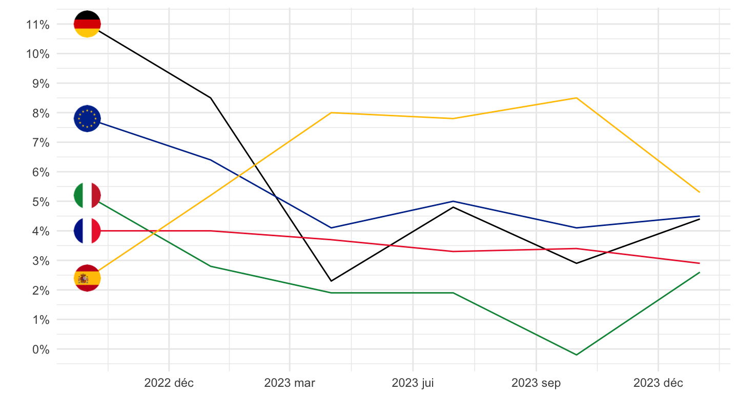
D1_D4_MD5 - Labour cost for LCI
France, Germany, Italy, Spain
All
Code
lc_lci_r2_q %>%
  filter(nace_r2 == "B-S",
         unit == "PCH_SM",
         lcstruct == "D1_D4_MD5",
         s_adj == "CA",
         geo %in% c("FR", "DE", "ES", "IT", "EA19")) %>%
  quarter_to_date %>%

  left_join(colors, by = c("Geo" = "country")) %>%
  mutate(values = values/100,
         Geo = ifelse(geo == "EA19", "Europe", Geo)) %>%
  ggplot(.) + geom_line(aes(x = date, y = values, color = color)) +
  theme_minimal() + xlab("") + ylab("") +
  scale_x_date(breaks = seq(1960, 2100, 2) %>% paste0("-01-01") %>% as.Date,
               labels = date_format("%Y")) +
  scale_y_continuous(breaks = 0.01*seq(-20, 20, 1),
                     labels = percent_format(a = 1)) +
  scale_color_identity() + add_flags +
  theme(legend.position = c(0.75, 0.90),
        legend.title = element_blank())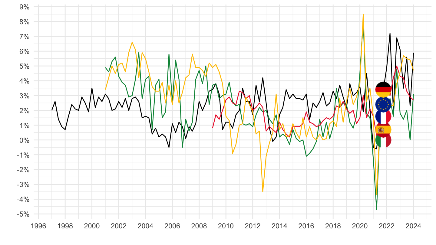
2017-
Code
lc_lci_r2_q %>%
  filter(nace_r2 == "B-S",
         unit == "PCH_SM",
         lcstruct == "D1_D4_MD5",
         s_adj == "CA",
         geo %in% c("FR", "DE", "ES", "IT")) %>%
  quarter_to_date %>%
  filter(date >= as.Date("2017-01-01")) %>%

  left_join(colors, by = c("Geo" = "country")) %>%
  mutate(values = values/100) %>%
  ggplot(.) + geom_line(aes(x = date, y = values, color = color)) +
  theme_minimal() + xlab("") + ylab("") +
  scale_x_date(breaks = seq(1960, 2100, 1) %>% paste0("-01-01") %>% as.Date,
               labels = date_format("%Y")) +
  scale_y_continuous(breaks = 0.01*seq(-20, 20, 1),
                     labels = percent_format(a = 1)) +
  scale_color_identity() + add_flags +
  theme(legend.position = c(0.75, 0.90),
        legend.title = element_blank())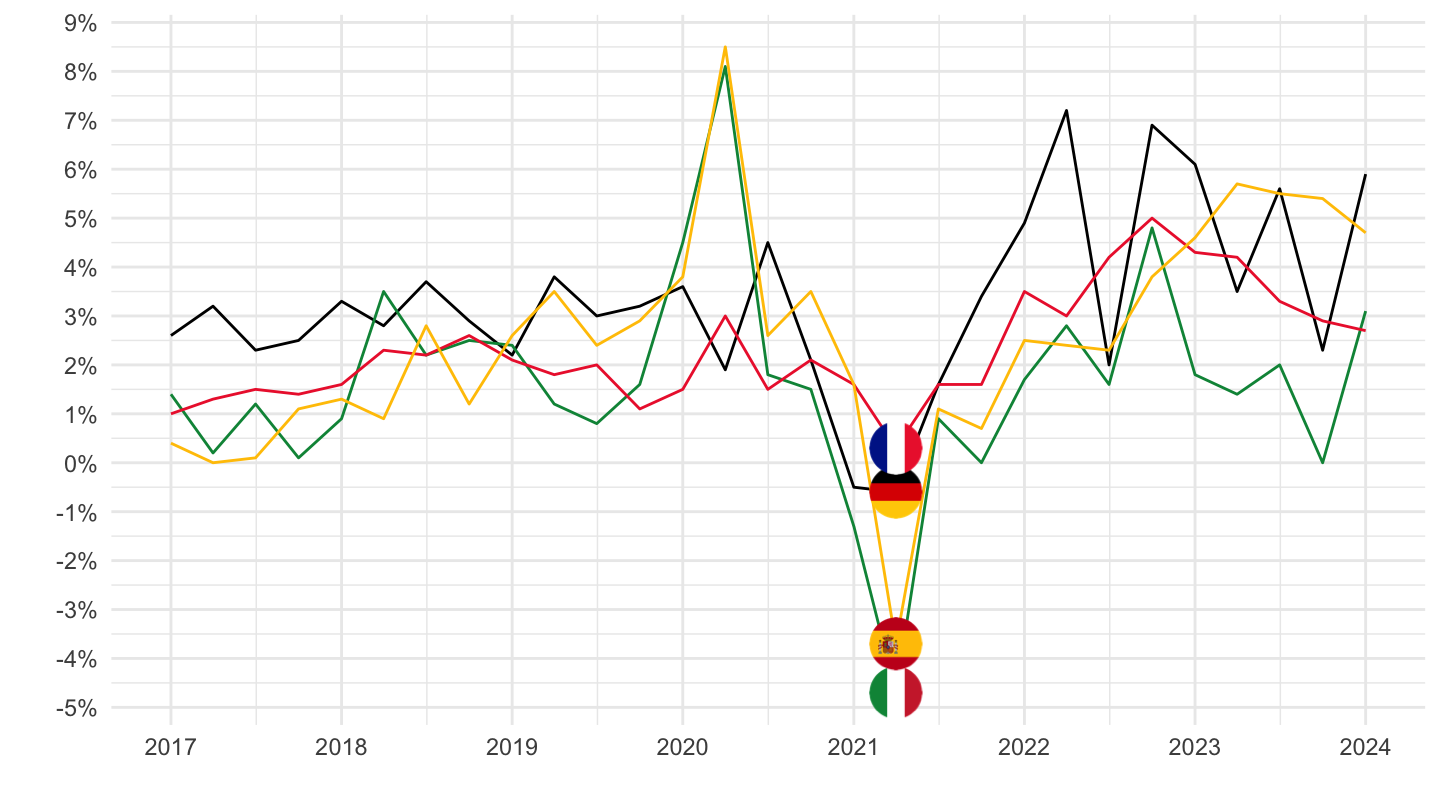
2020-
Code
lc_lci_r2_q %>%
  filter(nace_r2 == "B-S",
         unit == "PCH_SM",
         lcstruct == "D1_D4_MD5",
         s_adj == "CA",
         geo %in% c("FR", "DE", "ES", "IT", "EA19")) %>%
  quarter_to_date %>%
  filter(date >= as.Date("2020-01-01")) %>%

  mutate(values = values/100,
         Geo = ifelse(geo == "EA19", "Europe", Geo)) %>%
  left_join(colors, by = c("Geo" = "country")) %>%
  ggplot(.) + geom_line(aes(x = date, y = values, color = color)) +
  theme_minimal() + xlab("") + ylab("") +
  scale_x_date(breaks = "6 months",
               labels = date_format("%Y %b")) +
  scale_y_continuous(breaks = 0.01*seq(-20, 20, 1),
                     labels = percent_format(a = 1)) +
  scale_color_identity() + add_flags +
  theme(legend.position = c(0.75, 0.90),
        legend.title = element_blank())