Unit labour costs and labour productivity (employment based), Total economy
Data - OECD
Info
Data on productivity
Data on wages
| source | dataset | Title | .html | .rData |
|---|---|---|---|---|
| eurostat | earn_mw_cur | Monthly minimum wages - bi-annual data | 2026-06-03 | 2026-04-26 |
| eurostat | ei_lmlc_q | Labour cost index, nominal value - quarterly data | 2026-06-03 | 2026-04-26 |
| eurostat | lc_lci_lev | Labour cost levels by NACE Rev. 2 activity | 2026-06-03 | 2026-04-26 |
| eurostat | lc_lci_r2_q | Labour cost index by NACE Rev. 2 activity - nominal value, quarterly data | 2026-06-03 | 2026-05-28 |
| eurostat | nama_10_lp_ulc | Labour productivity and unit labour costs | 2026-06-04 | 2026-04-26 |
| eurostat | namq_10_lp_ulc | Labour productivity and unit labour costs | 2026-06-04 | 2026-04-26 |
| eurostat | tps00155 | Minimum wages | 2026-06-04 | 2026-04-26 |
| fred | wage | Wage | 2026-06-04 | 2026-05-29 |
| ilo | EAR_4MTH_SEX_ECO_CUR_NB_A | Mean nominal monthly earnings of employees by sex and economic activity -- Harmonized series | 2024-06-20 | 2023-06-01 |
| ilo | EAR_XEES_SEX_ECO_NB_Q | Mean nominal monthly earnings of employees by sex and economic activity -- Harmonized series | 2024-06-20 | 2023-06-01 |
| oecd | AV_AN_WAGE | Average annual wages | 2026-06-04 | 2026-06-04 |
| oecd | AWCOMP | Taxing Wages - Comparative tables | 2026-06-04 | 2023-09-09 |
| oecd | EAR_MEI | Hourly Earnings (MEI) | 2026-06-04 | 2024-04-16 |
| oecd | HH_DASH | Household Dashboard | 2026-06-04 | 2023-09-09 |
| oecd | MIN2AVE | Minimum relative to average wages of full-time workers - MIN2AVE | 2026-02-22 | 2023-09-09 |
| oecd | RMW | Real Minimum Wages - RMW | 2026-06-04 | 2024-03-12 |
| oecd | ULC_EEQ | Unit labour costs and labour productivity (employment based), Total economy | 2026-06-04 | 2024-04-15 |
LAST_COMPILE
| LAST_COMPILE |
|---|
| 2026-06-21 |
Last
| obsTime | FREQUENCY | Nobs |
|---|---|---|
| 2023 | A | 4 |
| 2022 | A | 138 |
| 2021 | A | 138 |
| 2023-Q4 | Q | 27 |
| 2023-Q3 | Q | 359 |
| 2023-Q2 | Q | 393 |
Number of observations
Code
ULC_EEQ %>%
  left_join(ULC_EEQ_var$SUBJECT, by = c("SUBJECT")) %>%
  group_by(SUBJECT, Subject, MEASURE, FREQUENCY) %>%
  summarise(Nobs = n()) %>%
  arrange(-Nobs) %>%
  {if (is_html_output()) datatable(., filter = 'top', rownames = F) else .}
Data Structure
Code
ULC_EEQ_var$VAR_DESC %>%
{if (is_html_output()) print_table(.) else .}| id | description |
|---|---|
| LOCATION | Country |
| SUBJECT | Subject |
| MEASURE | Measure |
| FREQUENCY | Frequency |
| TIME | Time |
| OBS_VALUE | Observation Value |
| TIME_FORMAT | Time Format |
| OBS_STATUS | Observation Status |
| UNIT | Unit |
| POWERCODE | Unit multiplier |
| REFERENCEPERIOD | Reference period |
SUBJECT
Code
ULC_EEQ %>%
  left_join(ULC_EEQ_var$SUBJECT, by = "SUBJECT") %>%
  group_by(SUBJECT, Subject) %>%
  summarise(Nobs = n()) %>%
  arrange(-Nobs) %>%
{if (is_html_output()) print_table(.) else .}| SUBJECT | Subject | Nobs |
|---|---|---|
| ULQEUL01 | Unit Labour Costs | 22408 |
| ULQELP01 | GDP per person employed | 18962 |
| ULQECU01 | Labour Compensation per employed person | 18189 |
MEASURE
Code
ULC_EEQ %>%
  left_join(ULC_EEQ_var$MEASURE, by = "MEASURE") %>%
  group_by(MEASURE, Measure) %>%
  summarise(Nobs = n()) %>%
  arrange(-Nobs) %>%
{if (is_html_output()) print_table(.) else .}| MEASURE | Measure | Nobs |
|---|---|---|
| IXOBSA | Index, seasonally adjusted | 15645 |
| GPSA | Quarterly change compared to previous quarter, seasonally adjusted | 15421 |
| GYSA | Quarterly change on the same quarter of the previous year, seasonally adjusted | 15161 |
| IXOB | Index | 13332 |
FREQUENCY
Code
ULC_EEQ %>%
  left_join(ULC_EEQ_var$FREQUENCY, by = "FREQUENCY") %>%
  group_by(FREQUENCY, Frequency) %>%
  summarise(Nobs = n()) %>%
  arrange(-Nobs) %>%
{if (is_html_output()) print_table(.) else .}| FREQUENCY | Frequency | Nobs |
|---|---|---|
| Q | Quarterly | 55045 |
| A | Annual | 4514 |
TIME_FORMAT
Code
ULC_EEQ %>%
  left_join(ULC_EEQ_var$TIME_FORMAT, by = "TIME_FORMAT") %>%
  group_by(TIME_FORMAT, Time_format) %>%
  summarise(Nobs = n()) %>%
  arrange(-Nobs) %>%
{if (is_html_output()) print_table(.) else .}| TIME_FORMAT | Time_format | Nobs |
|---|---|---|
| P3M | Quarterly | 55045 |
| P1Y | Annual | 4514 |
LOCATION
Code
ULC_EEQ %>%
  left_join(ULC_EEQ_var$LOCATION, by = "LOCATION") %>%
  group_by(LOCATION, Location) %>%
  summarise(Nobs = n()) %>%
  arrange(-Nobs) %>%
  {if (is_html_output()) datatable(., filter = 'top', rownames = F) else .}
Unit Labour Cost
France / Germany
Code
ULC_EEQ %>%
  filter(MEASURE == "IXOBSA",
         SUBJECT == "ULQEUL01",
         LOCATION %in% c("FRA", "DEU"),
         FREQUENCY == "Q") %>%
  left_join(ULC_EEQ_var$LOCATION, by = "LOCATION") %>%
  quarter_to_date %>%
  ggplot() + geom_line(aes(x = date, y = obsValue, color = Location)) +

  theme_minimal() +
  scale_x_date(breaks = seq(1920, 2100, 5) %>% paste0("-01-01") %>% as.Date,
               labels = date_format("%Y")) +
  theme(legend.position = c(0.8, 0.2),
        legend.title = element_blank()) +
  scale_y_continuous(breaks = seq(0, 200, 10)) +
  ylab("Unit Labour Cost") + xlab("")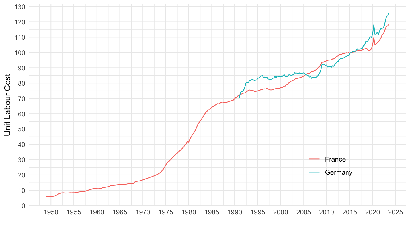
France / Germany from 1990
Code
ULC_EEQ %>%
  filter(MEASURE == "IXOBSA",
         SUBJECT == "ULQEUL01",
         LOCATION %in% c("FRA", "DEU"),
         FREQUENCY == "Q") %>%
  left_join(ULC_EEQ_var$LOCATION, by = "LOCATION") %>%
  quarter_to_date %>%
  filter(year(date) >= 1990) %>%
  left_join(colors, by = c("Location" = "country")) %>%
  ggplot() + geom_line(aes(x = date, y = obsValue, color = color)) +
  theme_minimal() + ylab("GDP per person employed") + xlab("") + add_2flags +
  scale_x_date(breaks = seq(1920, 2100, 2) %>% paste0("-01-01") %>% as.Date,
               labels = date_format("%Y")) +
  scale_color_identity() +
  theme(legend.position = c(0.8, 0.2),
        legend.title = element_blank()) +
  scale_y_continuous(breaks = seq(0, 200, 5))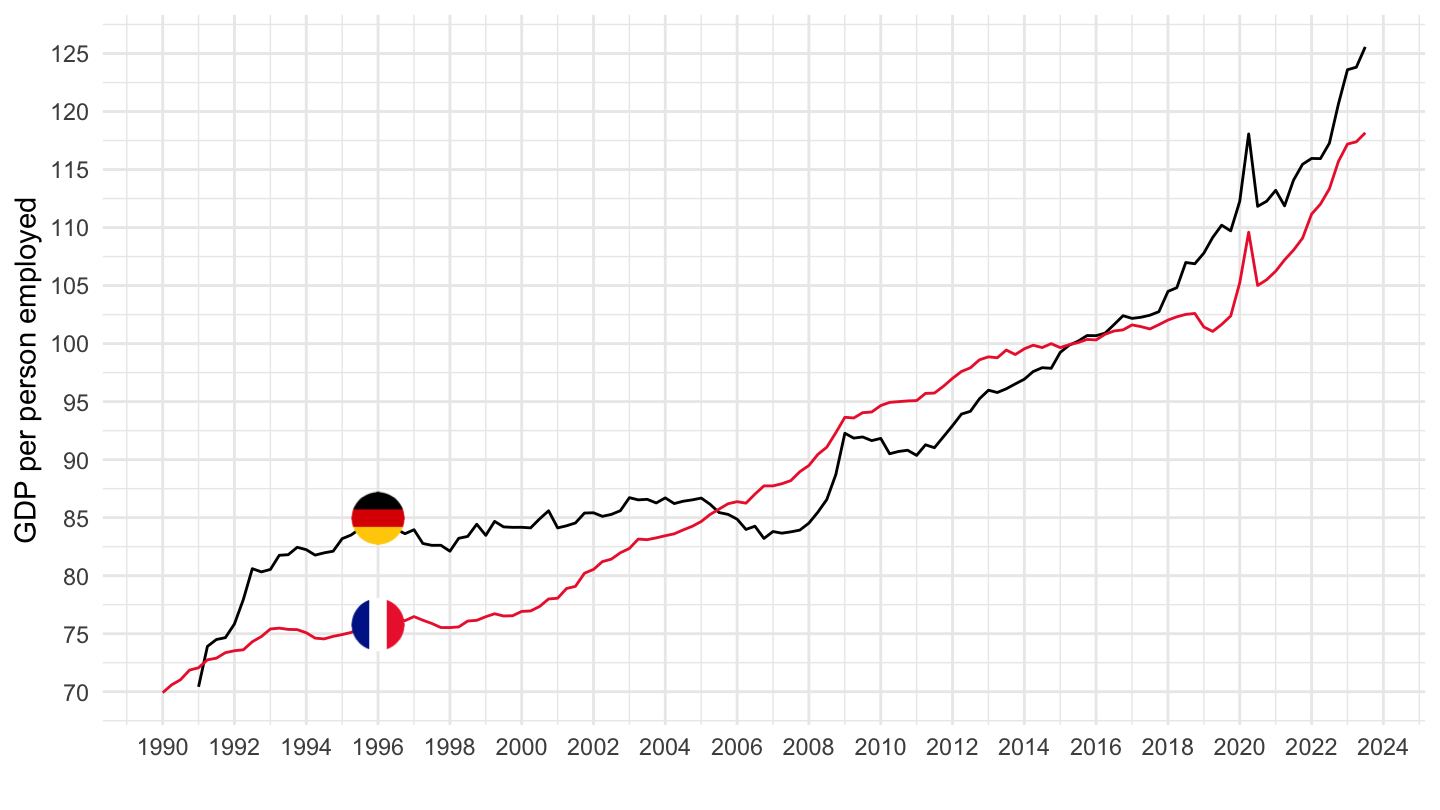
France / Germany / United States
Unit Labour Costs - ULQEUL01
Code
ULC_EEQ %>%
  filter(MEASURE == "IXOBSA",
         SUBJECT == "ULQEUL01",
         LOCATION %in% c("FRA", "DEU", "USA"),
         FREQUENCY == "Q") %>%
  left_join(ULC_EEQ_var$LOCATION, by = "LOCATION") %>%
  quarter_to_date %>%
  filter(year(date) >= 1990) %>%
  group_by(Location) %>%
  mutate(obsValue = 100*obsValue/obsValue[date == as.Date("1996-01-01")]) %>%
  left_join(colors, by = c("Location" = "country")) %>%
  ggplot() + geom_line(aes(x = date, y = obsValue, color = color)) +
  theme_minimal() + ylab("GDP per person employed") + xlab("") + add_3flags +
  scale_x_date(breaks = seq(1920, 2100, 2) %>% paste0("-01-01") %>% as.Date,
               labels = date_format("%Y")) +
  scale_color_identity() +
  theme(legend.position = c(0.8, 0.2),
        legend.title = element_blank()) +
  scale_y_continuous(breaks = seq(0, 200, 5))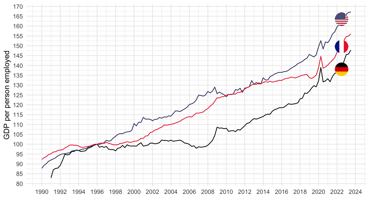
GDP per person employed - ULQELP01
Code
ULC_EEQ %>%
  filter(MEASURE == "IXOBSA",
         SUBJECT == "ULQELP01",
         LOCATION %in% c("FRA", "DEU", "USA"),
         FREQUENCY == "Q") %>%
  left_join(ULC_EEQ_var$LOCATION, by = "LOCATION") %>%
  quarter_to_date %>%
  filter(year(date) >= 1990) %>%
  group_by(Location) %>%
  mutate(obsValue = 100*obsValue/obsValue[date == as.Date("1996-01-01")]) %>%
  left_join(colors, by = c("Location" = "country")) %>%
  ggplot() + geom_line(aes(x = date, y = obsValue, color = color)) +
  theme_minimal() + ylab("GDP per person employed") + xlab("") + add_3flags +
  scale_x_date(breaks = seq(1920, 2100, 2) %>% paste0("-01-01") %>% as.Date,
               labels = date_format("%Y")) +
  scale_color_identity() +
  theme(legend.position = c(0.8, 0.2),
        legend.title = element_blank()) +
  scale_y_continuous(breaks = seq(0, 200, 5))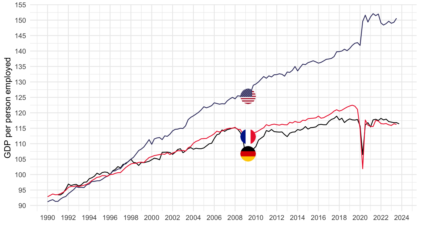
Labour Compensation per employed person - ULQECU01
Code
ULC_EEQ %>%
  filter(MEASURE == "IXOBSA",
         SUBJECT == "ULQECU01",
         LOCATION %in% c("FRA", "DEU", "USA"),
         FREQUENCY == "Q") %>%
  left_join(ULC_EEQ_var$LOCATION, by = "LOCATION") %>%
  quarter_to_date %>%
  filter(year(date) >= 1990) %>%
  group_by(Location) %>%
  mutate(obsValue = 100*obsValue/obsValue[date == as.Date("1996-01-01")]) %>%
  left_join(colors, by = c("Location" = "country")) %>%
  ggplot() + geom_line(aes(x = date, y = obsValue, color = color)) +
  theme_minimal() + ylab("Labour Compensation per employed person") + xlab("") + add_3flags +
  scale_x_date(breaks = seq(1920, 2100, 2) %>% paste0("-01-01") %>% as.Date,
               labels = date_format("%Y")) +
  scale_color_identity() +
  theme(legend.position = c(0.8, 0.2),
        legend.title = element_blank()) +
  scale_y_continuous(breaks = seq(0, 300, 10))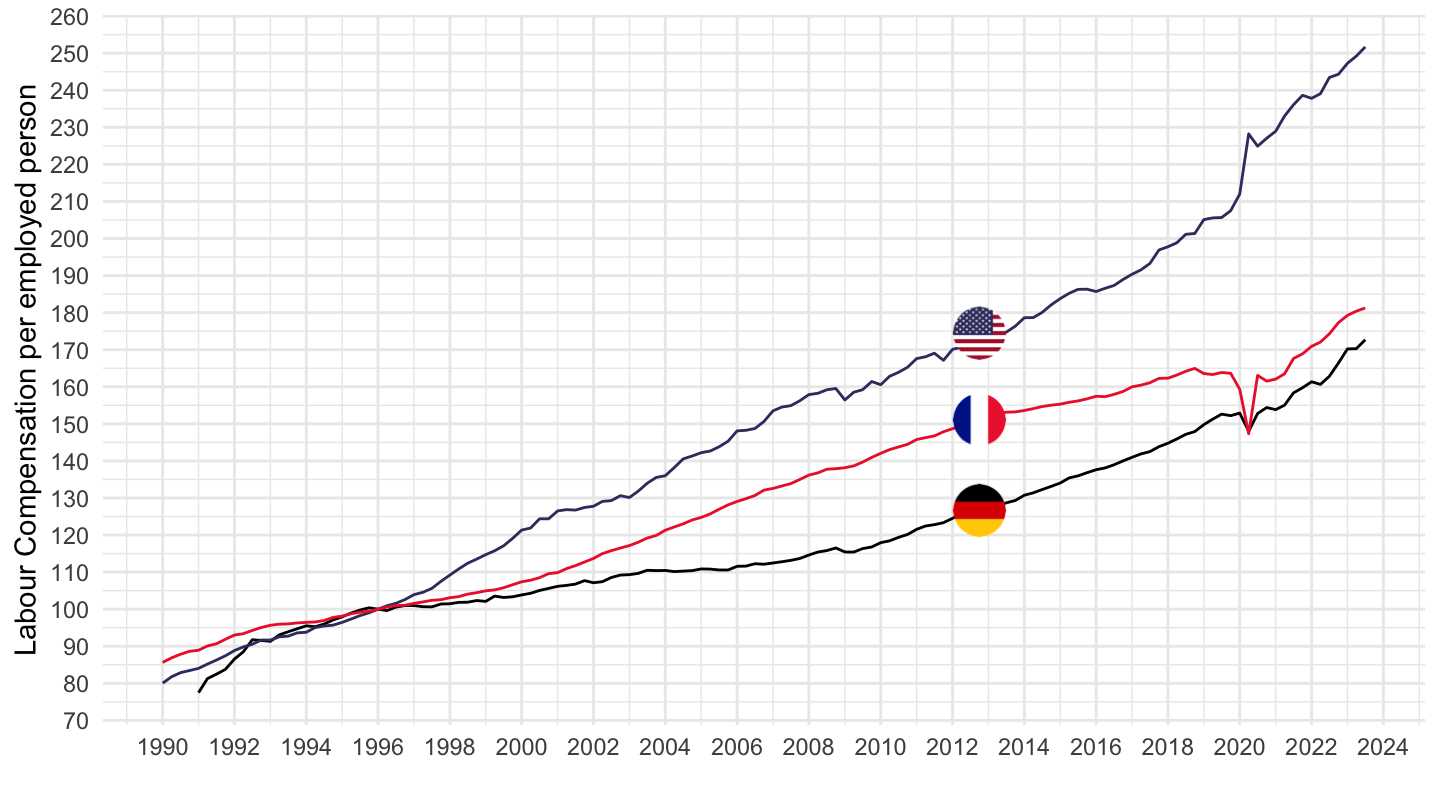
Euro area / United States
Unit Labour Costs - ULQEUL01
All
Code
ULC_EEQ %>%
  filter(MEASURE == "IXOBSA",
         SUBJECT == "ULQEUL01",
         LOCATION %in% c("EA19", "USA"),
         FREQUENCY == "Q") %>%
  left_join(ULC_EEQ_var$LOCATION, by = "LOCATION") %>%
  quarter_to_date %>%
  filter(year(date) >= 1990) %>%
  group_by(Location) %>%
  mutate(obsValue = 100*obsValue/obsValue[date == as.Date("1996-01-01")]) %>%
  mutate(Location = ifelse(LOCATION == "EA19", "Europe", Location)) %>%
  left_join(colors, by = c("Location" = "country")) %>%
  mutate(color = ifelse(LOCATION == "USA", color2, color)) %>%
  ggplot() + geom_line(aes(x = date, y = obsValue, color = color)) +
  theme_minimal() + ylab("Unit Labour Cost") + xlab("") + add_2flags +
  scale_x_date(breaks = seq(1920, 2100, 2) %>% paste0("-01-01") %>% as.Date,
               labels = date_format("%Y")) +
  scale_color_identity() +
  theme(legend.position = c(0.8, 0.2),
        legend.title = element_blank()) +
  scale_y_log10(breaks = seq(0, 200, 5))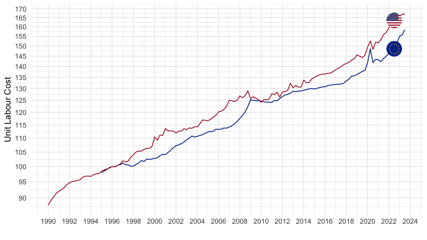
1995-
Code
ULC_EEQ %>%
  filter(MEASURE == "IXOBSA",
         SUBJECT == "ULQEUL01",
         LOCATION %in% c("EA19", "USA"),
         FREQUENCY == "Q") %>%
  left_join(ULC_EEQ_var$LOCATION, by = "LOCATION") %>%
  quarter_to_date %>%
  filter(year(date) >= 1995) %>%
  group_by(Location) %>%
  mutate(obsValue = 100*obsValue/obsValue[date == as.Date("1995-01-01")]) %>%
  mutate(Location = ifelse(LOCATION == "EA19", "Europe", Location)) %>%
  left_join(colors, by = c("Location" = "country")) %>%
  mutate(color = ifelse(LOCATION == "USA", color2, color)) %>%
  ggplot() + geom_line(aes(x = date, y = obsValue, color = color)) +
  theme_minimal() + ylab("Unit Labour Cost") + xlab("") + add_2flags +
  scale_x_date(breaks = seq(1921, 2100, 2) %>% paste0("-01-01") %>% as.Date,
               labels = date_format("%Y")) +
  scale_color_identity() +
  theme(legend.position = c(0.8, 0.2),
        legend.title = element_blank()) +
  scale_y_log10(breaks = seq(0, 200, 5))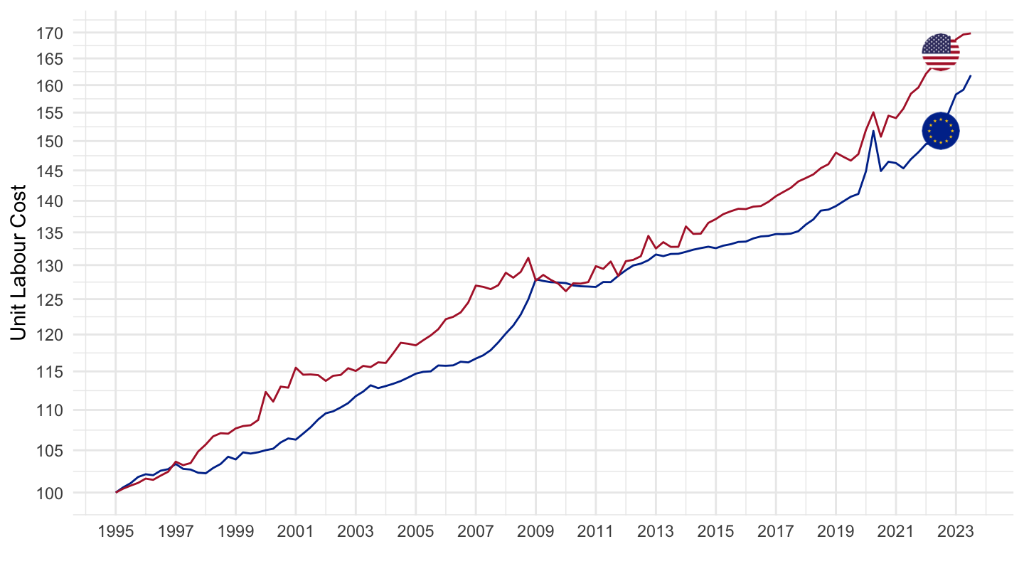
1996-
Code
ULC_EEQ %>%
  filter(MEASURE == "IXOBSA",
         SUBJECT == "ULQEUL01",
         LOCATION %in% c("EA19", "USA"),
         FREQUENCY == "Q") %>%
  left_join(ULC_EEQ_var$LOCATION, by = "LOCATION") %>%
  quarter_to_date %>%
  filter(year(date) >= 1996) %>%
  group_by(Location) %>%
  mutate(obsValue = 100*obsValue/obsValue[date == as.Date("1996-01-01")]) %>%
  mutate(Location = ifelse(LOCATION == "EA19", "Europe", Location)) %>%
  left_join(colors, by = c("Location" = "country")) %>%
  mutate(color = ifelse(LOCATION == "USA", color2, color)) %>%
  ggplot() + geom_line(aes(x = date, y = obsValue, color = color)) +
  theme_minimal() + ylab("Unit Labour Cost") + xlab("") + add_2flags +
  scale_x_date(breaks = seq(1920, 2100, 2) %>% paste0("-01-01") %>% as.Date,
               labels = date_format("%Y")) +
  scale_color_identity() +
  theme(legend.position = c(0.8, 0.2),
        legend.title = element_blank()) +
  scale_y_log10(breaks = seq(0, 200, 5))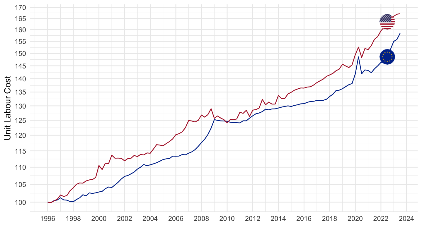
2017-
Code
ULC_EEQ %>%
  filter(MEASURE == "IXOBSA",
         SUBJECT == "ULQEUL01",
         LOCATION %in% c("EA19", "USA"),
         FREQUENCY == "Q") %>%
  left_join(ULC_EEQ_var$LOCATION, by = "LOCATION") %>%
  quarter_to_date %>%
  filter(year(date) >= 2017) %>%
  group_by(Location) %>%
  mutate(obsValue = 100*obsValue/obsValue[date == as.Date("2017-01-01")]) %>%
  mutate(Location = ifelse(LOCATION == "EA19", "Europe", Location)) %>%
  left_join(colors, by = c("Location" = "country")) %>%
  mutate(color = ifelse(LOCATION == "USA", color2, color)) %>%
  ggplot() + geom_line(aes(x = date, y = obsValue, color = color)) +

  theme_minimal() + ylab("Unit Labour Cost") + xlab("") + add_2flags +
  scale_x_date(breaks = seq(1920, 2100, 1) %>% paste0("-01-01") %>% as.Date,
               labels = date_format("%Y")) +
  scale_color_identity() +
  theme(legend.position = c(0.8, 0.2),
        legend.title = element_blank()) +
  scale_y_continuous(breaks = seq(0, 200, 5))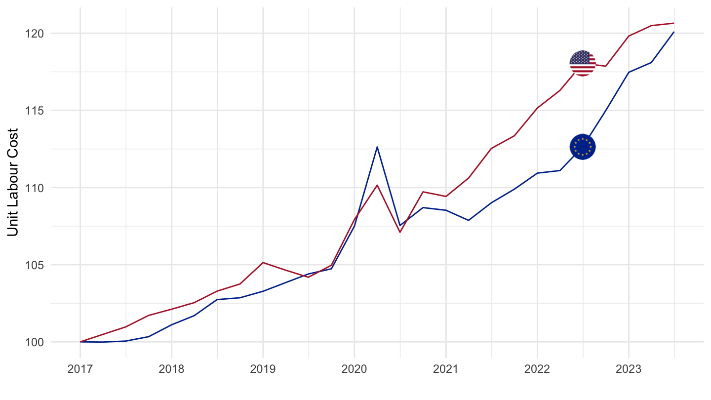
2020-
Code
ULC_EEQ %>%
  filter(MEASURE == "IXOBSA",
         SUBJECT == "ULQEUL01",
         LOCATION %in% c("EA19", "USA"),
         FREQUENCY == "Q") %>%
  left_join(ULC_EEQ_var$LOCATION, by = "LOCATION") %>%
  quarter_to_date %>%
  filter(year(date) >= 2020) %>%
  group_by(Location) %>%
  mutate(obsValue = 100*obsValue/obsValue[date == as.Date("2020-01-01")]) %>%
  mutate(Location = ifelse(LOCATION == "EA19", "Europe", Location)) %>%
  left_join(colors, by = c("Location" = "country")) %>%
  mutate(color = ifelse(LOCATION == "USA", color2, color)) %>%
  ggplot() + geom_line(aes(x = date, y = obsValue, color = color)) +

  theme_minimal() + ylab("Unit Labour Cost") + xlab("") + add_2flags +
  scale_x_date(breaks = seq(1920, 2100, 1) %>% paste0("-01-01") %>% as.Date,
               labels = date_format("%Y")) +
  scale_color_identity() +
  theme(legend.position = c(0.8, 0.2),
        legend.title = element_blank()) +
  scale_y_continuous(breaks = seq(0, 200, 5))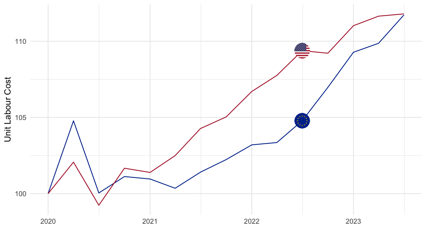
GDP per person employed - ULQELP01
All
Code
ULC_EEQ %>%
  filter(MEASURE == "IXOBSA",
         SUBJECT == "ULQELP01",
         LOCATION %in% c("EA19", "USA"),
         FREQUENCY == "Q") %>%
  left_join(ULC_EEQ_var$LOCATION, by = "LOCATION") %>%
  quarter_to_date %>%
  filter(year(date) >= 1990) %>%
  group_by(Location) %>%
  mutate(obsValue = 100*obsValue/obsValue[date == as.Date("1996-01-01")]) %>%
  ggplot() + geom_line(aes(x = date, y = obsValue, color = Location)) +

  theme_minimal() + ylab("GDP per person employed") + xlab("") +
  scale_x_date(breaks = seq(1920, 2100, 2) %>% paste0("-01-01") %>% as.Date,
               labels = date_format("%Y")) +
  theme(legend.position = c(0.8, 0.2),
        legend.title = element_blank()) +
  scale_y_continuous(breaks = seq(0, 200, 5))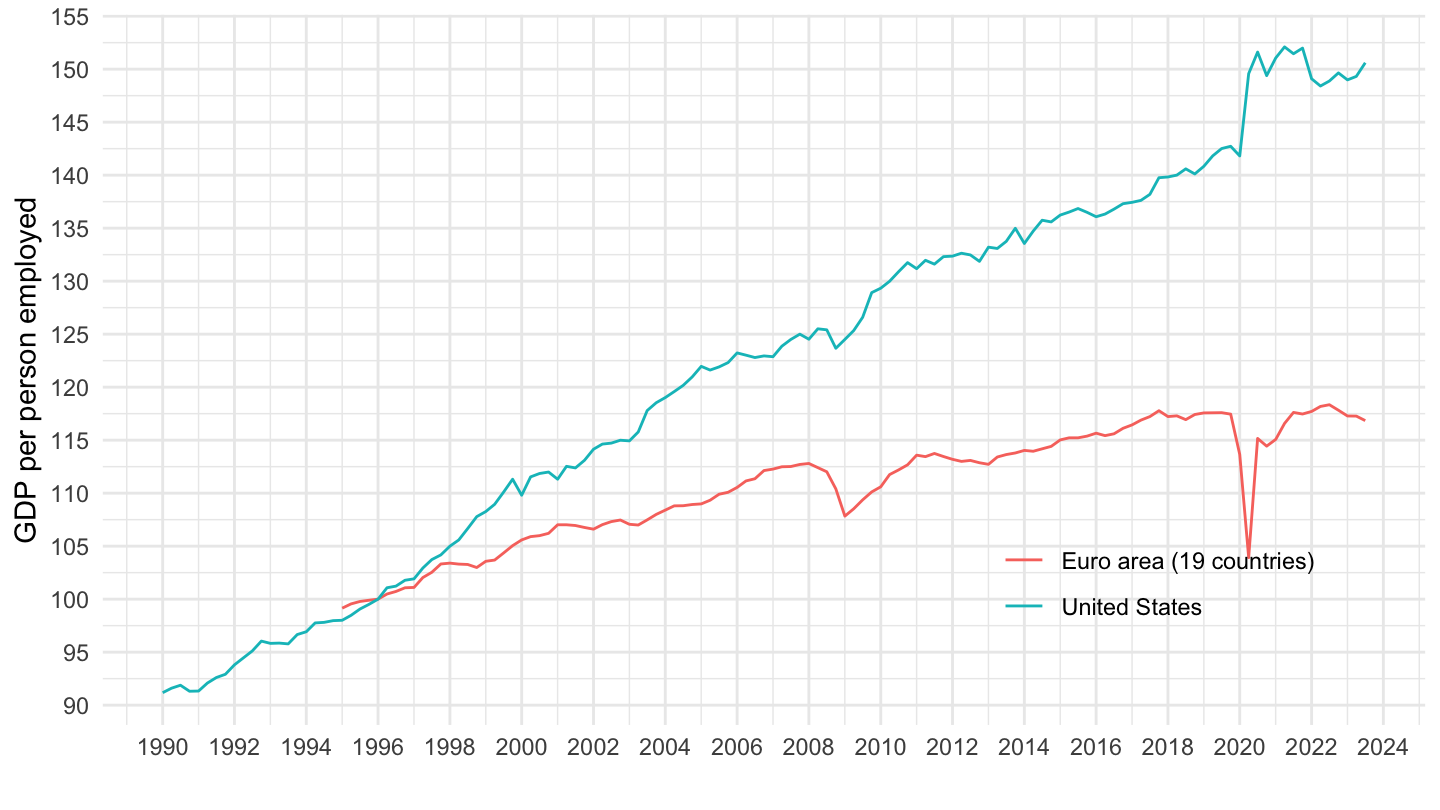
2017-
Code
ULC_EEQ %>%
  filter(MEASURE == "IXOBSA",
         SUBJECT == "ULQELP01",
         LOCATION %in% c("EA19", "USA"),
         FREQUENCY == "Q") %>%
  left_join(ULC_EEQ_var$LOCATION, by = "LOCATION") %>%
  quarter_to_date %>%
  filter(year(date) >= 2017) %>%
  group_by(Location) %>%
  mutate(obsValue = 100*obsValue/obsValue[date == as.Date("2017-01-01")]) %>%
  mutate(Location = ifelse(LOCATION == "EA19", "Europe", Location)) %>%
  left_join(colors, by = c("Location" = "country")) %>%
  mutate(color = ifelse(LOCATION == "USA", color2, color)) %>%
  ggplot() + geom_line(aes(x = date, y = obsValue, color = color)) +

  theme_minimal() + ylab("Unit Labour Cost") + xlab("") + add_2flags +
  scale_x_date(breaks = seq(1920, 2100, 1) %>% paste0("-01-01") %>% as.Date,
               labels = date_format("%Y")) +
  scale_color_identity() +
  theme(legend.position = c(0.8, 0.2),
        legend.title = element_blank()) +
  scale_y_continuous(breaks = seq(0, 200, 5))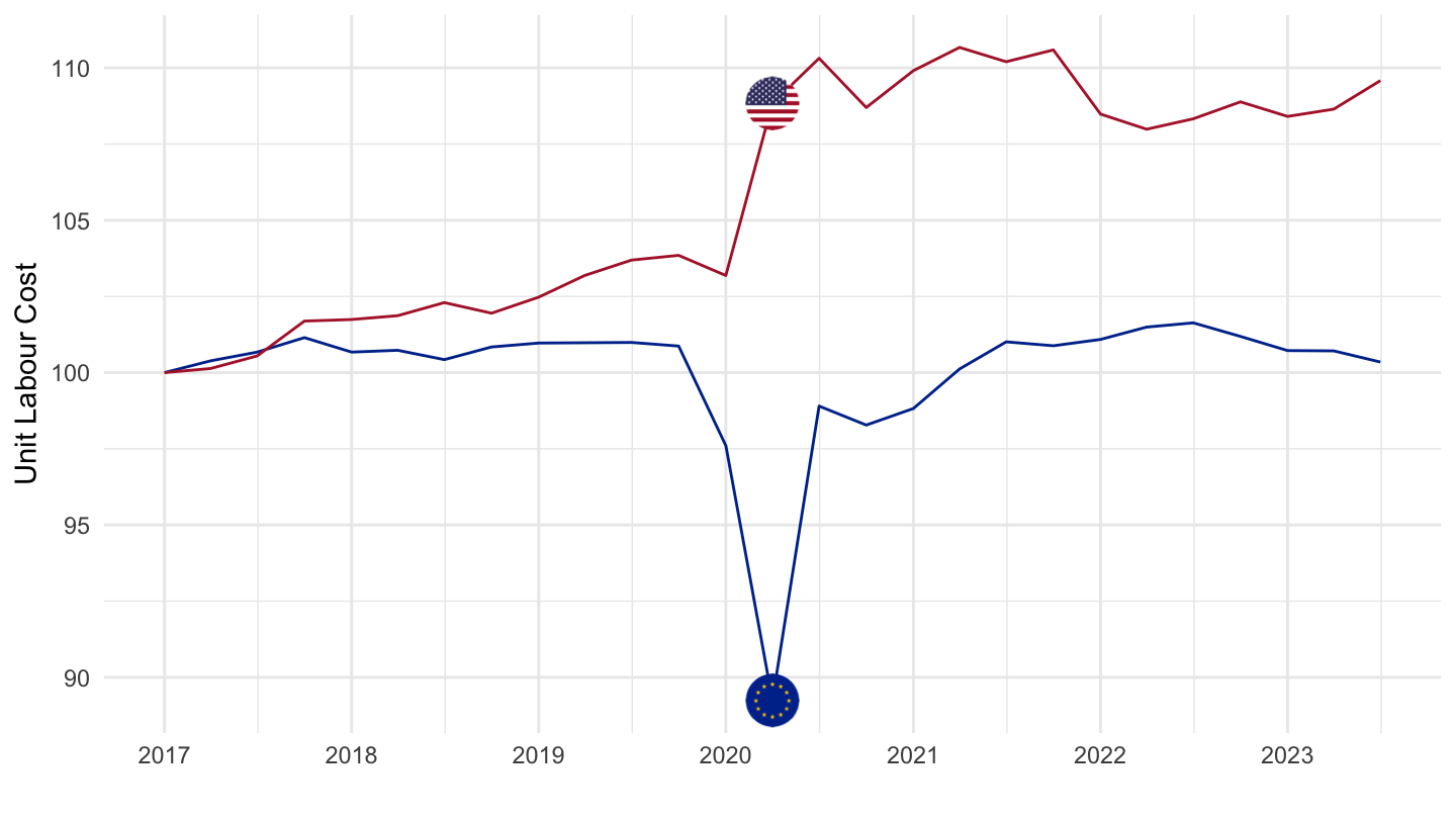
2020-
Code
ULC_EEQ %>%
  filter(MEASURE == "IXOBSA",
         SUBJECT == "ULQELP01",
         LOCATION %in% c("EA19", "USA"),
         FREQUENCY == "Q") %>%
  left_join(ULC_EEQ_var$LOCATION, by = "LOCATION") %>%
  quarter_to_date %>%
  filter(year(date) >= 2020) %>%
  group_by(Location) %>%
  mutate(obsValue = 100*obsValue/obsValue[date == as.Date("2020-01-01")]) %>%
  mutate(Location = ifelse(LOCATION == "EA19", "Europe", Location)) %>%
  left_join(colors, by = c("Location" = "country")) %>%
  mutate(color = ifelse(LOCATION == "USA", color2, color)) %>%
  ggplot() + geom_line(aes(x = date, y = obsValue, color = color)) +

  theme_minimal() + ylab("Unit Labour Cost") + xlab("") + add_2flags +
  scale_x_date(breaks = seq(1920, 2100, 1) %>% paste0("-01-01") %>% as.Date,
               labels = date_format("%Y")) +
  scale_color_identity() +
  theme(legend.position = c(0.8, 0.2),
        legend.title = element_blank()) +
  scale_y_continuous(breaks = seq(0, 200, 5))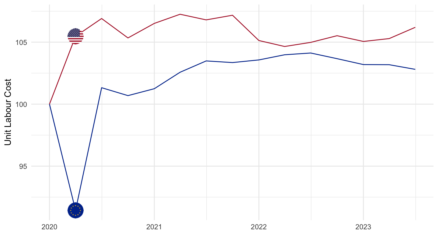
Labour Compensation per employed person - ULQECU01
All
Code
ULC_EEQ %>%
  filter(MEASURE == "IXOBSA",
         SUBJECT == "ULQECU01",
         LOCATION %in% c("EA19", "USA"),
         FREQUENCY == "Q") %>%
  left_join(ULC_EEQ_var$LOCATION, by = "LOCATION") %>%
  quarter_to_date %>%
  filter(year(date) >= 1990) %>%
  group_by(Location) %>%
  mutate(obsValue = 100*obsValue/obsValue[date == as.Date("1996-01-01")]) %>%
  ggplot() + geom_line(aes(x = date, y = obsValue, color = Location)) +

  theme_minimal() + ylab("Labour Compensation per employed person") + xlab("") +
  scale_x_date(breaks = seq(1920, 2100, 2) %>% paste0("-01-01") %>% as.Date,
               labels = date_format("%Y")) +
  theme(legend.position = c(0.8, 0.2),
        legend.title = element_blank()) +
  scale_y_continuous(breaks = seq(0, 300, 10))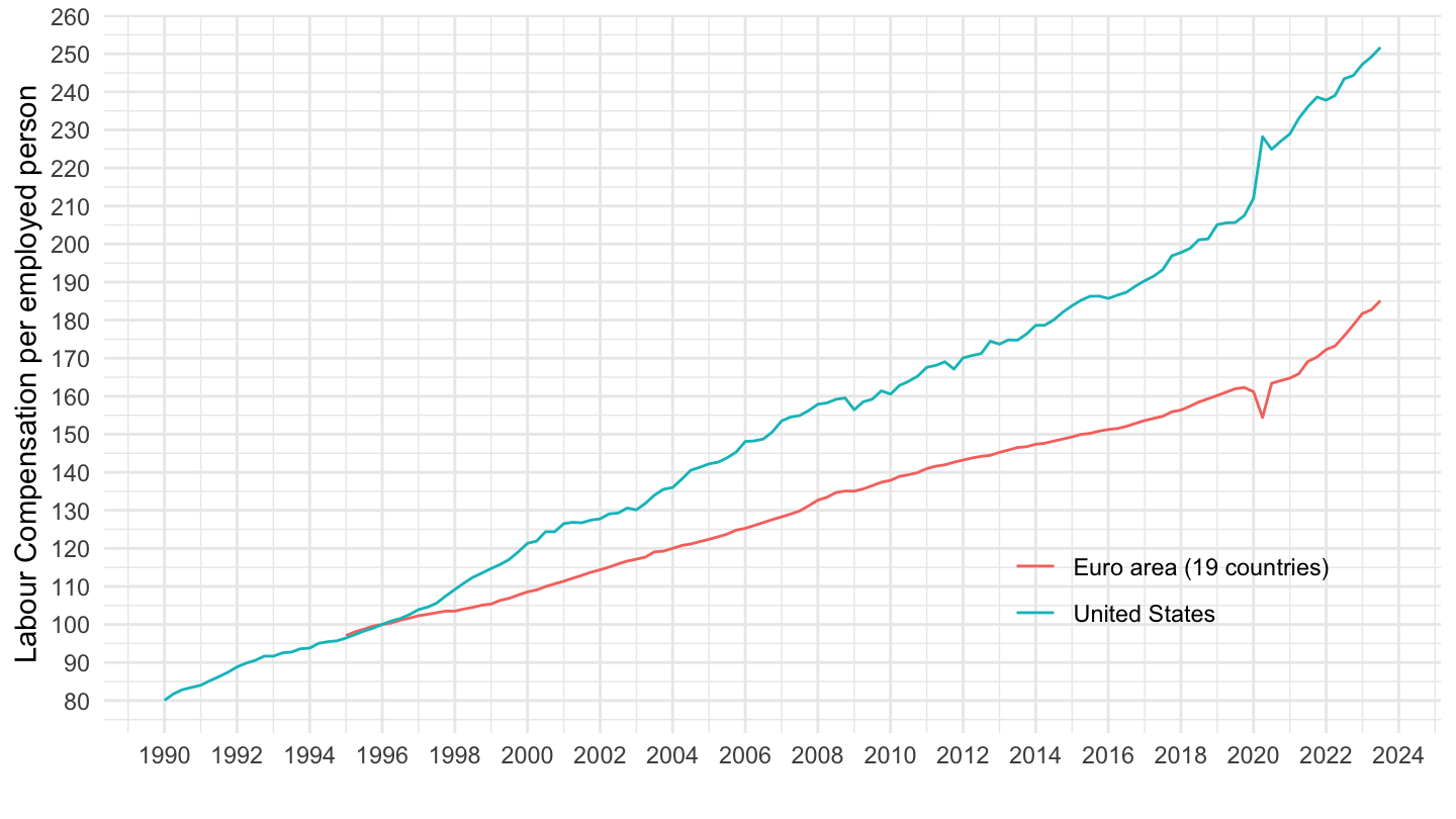
2017-
Code
ULC_EEQ %>%
  filter(MEASURE == "IXOBSA",
         SUBJECT == "ULQECU01",
         LOCATION %in% c("EA19", "USA"),
         FREQUENCY == "Q") %>%
  left_join(ULC_EEQ_var$LOCATION, by = "LOCATION") %>%
  quarter_to_date %>%
  filter(year(date) >= 2017) %>%
  group_by(Location) %>%
  mutate(obsValue = 100*obsValue/obsValue[date == as.Date("2017-01-01")]) %>%
  ggplot() + geom_line(aes(x = date, y = obsValue, color = Location)) +

  theme_minimal() + ylab("Labour Compensation per employed person") + xlab("") +
  scale_x_date(breaks = seq(1920, 2100, 1) %>% paste0("-01-01") %>% as.Date,
               labels = date_format("%Y")) +
  theme(legend.position = c(0.8, 0.2),
        legend.title = element_blank()) +
  scale_y_continuous(breaks = seq(0, 300, 10))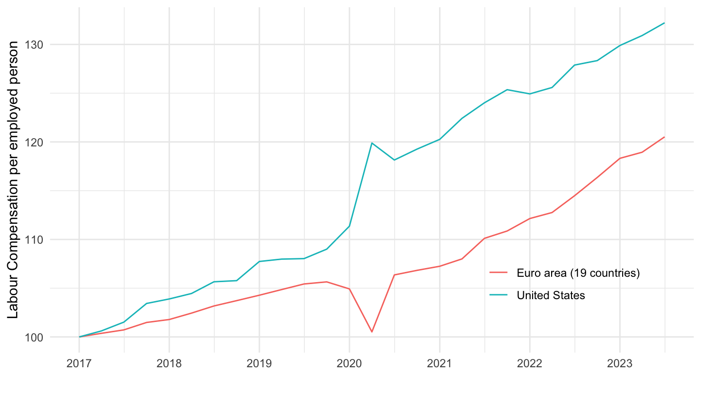
2019-Q4
Code
ULC_EEQ %>%
  filter(MEASURE == "IXOBSA",
         SUBJECT == "ULQECU01",
         LOCATION %in% c("EA19", "USA"),
         FREQUENCY == "Q") %>%
  mutate(Location = ifelse(LOCATION == "EA19", "Euro area", "US"),
         date = zoo::as.yearqtr(obsTime, format = "%Y-Q%q")) %>%
  filter(date >= zoo::as.yearqtr("2019 Q4")) %>%
  group_by(Location) %>%
  mutate(obsValue = 100*obsValue/obsValue[date == zoo::as.yearqtr("2019 Q4")]) %>%
  ggplot() + geom_line(aes(x = date, y = obsValue, color = Location)) +
  theme_minimal() + ylab("100 = 2019-Q4") + xlab("") +
  zoo::scale_x_yearqtr(format = "%Y-Q%q",
                       n = 15) +
  scale_color_manual(values = c("#003399", "#B22234")) +
  theme(legend.position = c(0.8, 0.2),
        legend.title = element_blank(),
        axis.text.x = element_text(angle = 45, hjust = 1)) +
  scale_y_continuous(breaks = seq(0, 300, 2))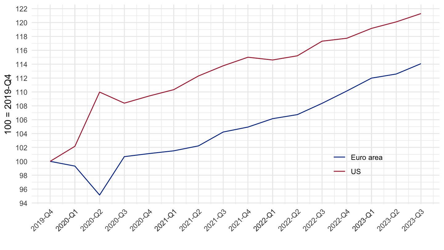
2020-
Code
ULC_EEQ %>%
  filter(MEASURE == "IXOBSA",
         SUBJECT == "ULQECU01",
         LOCATION %in% c("EA19", "USA"),
         FREQUENCY == "Q") %>%
  left_join(ULC_EEQ_var$LOCATION, by = "LOCATION") %>%
  quarter_to_date %>%
  filter(year(date) >= 2020) %>%
  group_by(Location) %>%
  mutate(obsValue = 100*obsValue/obsValue[date == as.Date("2020-01-01")]) %>%
  ggplot() + geom_line(aes(x = date, y = obsValue, color = Location)) +

  theme_minimal() + ylab("Labour Compensation per employed person") + xlab("") +
  scale_x_date(breaks = seq(1920, 2100, 1) %>% paste0("-01-01") %>% as.Date,
               labels = date_format("%Y")) +
  theme(legend.position = c(0.8, 0.2),
        legend.title = element_blank()) +
  scale_y_continuous(breaks = seq(0, 300, 2))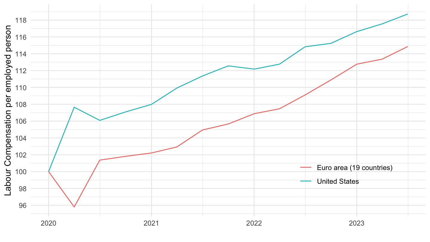
Euro area vs. US
2017-Q2
Code
ULC_EEQ %>%
  filter(MEASURE == "IXOBSA",
         LOCATION %in% c("EA19", "USA"),
         FREQUENCY == "Q") %>%
  left_join(ULC_EEQ_var$SUBJECT, by = "SUBJECT") %>%
  mutate(Subject = ifelse(SUBJECT == "ULQECU01", "Labour Compensation\nper person employed", Subject)) %>%
  mutate(Location = ifelse(LOCATION == "EA19", "Euro area", "US"),
         date = zoo::as.yearqtr(obsTime, format = "%Y-Q%q")) %>%
  filter(date >= zoo::as.yearqtr("2017 Q2")) %>%
  mutate(Subject = factor(Subject, levels = c("Unit Labour Costs ",
                                              "Labour Compensation\nper person employed",
                                              "GDP per person employed"))) %>%
  group_by(Location, Subject) %>%
  mutate(obsValue = 100*obsValue/obsValue[date == zoo::as.yearqtr("2017 Q2")]) %>%
  ggplot() + geom_line(aes(x = date, y = obsValue, color = Location)) +
  theme_minimal() + ylab("100 = 2019-Q4") + xlab("") +
  zoo::scale_x_yearqtr(format = "%Y-Q%q",
                       breaks = zoo::as.yearqtr(c("2017 Q2", "2017 Q4", "2018 Q2", "2018 Q4",
                                                  "2019 Q2", "2019 Q4", "2020 Q2", "2020 Q4",
                                                  "2021 Q2", "2021 Q4", "2022 Q2", "2022 Q4",
                                                  "2023 Q2"))) +
  scale_color_manual(values = c("#003399", "#B22234")) +
  theme(legend.position = "top",
        legend.title = element_blank(),
        axis.text.x = element_text(angle = 45, hjust = 1)) +
  scale_y_continuous(breaks = seq(0, 300, 2)) +
  facet_wrap(~ Subject)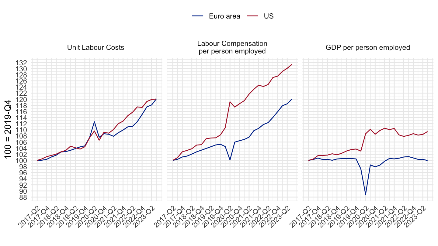
2019-Q4
Code
ULC_EEQ %>%
  filter(MEASURE == "IXOBSA",
         LOCATION %in% c("EA19", "USA"),
         FREQUENCY == "Q") %>%
  left_join(ULC_EEQ_var$SUBJECT, by = "SUBJECT") %>%
  mutate(Subject = ifelse(SUBJECT == "ULQECU01", "Labour Compensation\nper person employed", Subject)) %>%
  mutate(Location = ifelse(LOCATION == "EA19", "Euro area", "US"),
         date = zoo::as.yearqtr(obsTime, format = "%Y-Q%q")) %>%
  filter(date >= zoo::as.yearqtr("2019 Q4")) %>%
  mutate(Subject = factor(Subject, levels = c("Unit Labour Costs ",
                                              "Labour Compensation\nper person employed",
                                              "GDP per person employed"))) %>%
  group_by(Location, Subject) %>%
  mutate(obsValue = 100*obsValue/obsValue[date == zoo::as.yearqtr("2019 Q4")]) %>%
  ggplot() + geom_line(aes(x = date, y = obsValue, color = Location)) +
  theme_minimal() + ylab("100 = 2019-Q4") + xlab("") +
  zoo::scale_x_yearqtr(format = "%Y-Q%q",
                       breaks = zoo::as.yearqtr(c("2019 Q4", "2020 Q2", "2020 Q4",
                                                  "2021 Q2", "2021 Q4", "2022 Q2",
                                                  "2022 Q4", "2023 Q2"))) +
  scale_color_manual(values = c("#003399", "#B22234")) +
  theme(legend.position = "top",
        legend.title = element_blank(),
        axis.text.x = element_text(angle = 45, hjust = 1)) +
  scale_y_continuous(breaks = seq(0, 300, 2)) +
  facet_wrap(~ Subject)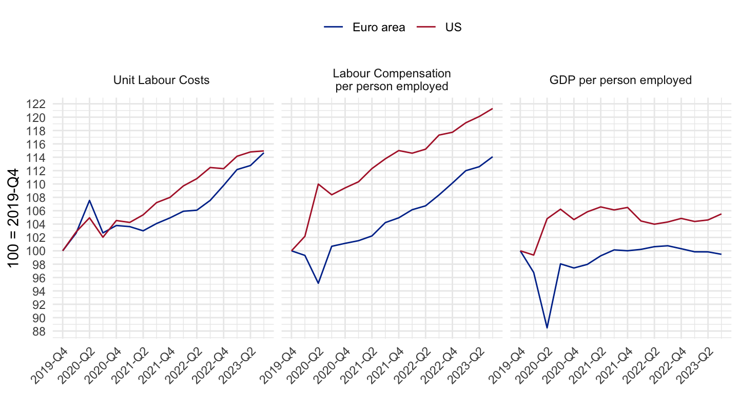
France, US, Eurozone
2019-Q4
Code
ULC_EEQ %>%
  filter(MEASURE == "IXOBSA",
         LOCATION %in% c("EA19", "USA", "FRA"),
         FREQUENCY == "Q") %>%
  left_join(ULC_EEQ_var$SUBJECT, by = "SUBJECT") %>%
  mutate(Subject = ifelse(SUBJECT == "ULQECU01", "Labour Compensation\nper person employed", Subject)) %>%
  mutate(Location = case_when(LOCATION == "EA19" ~ "Euro area",
                              LOCATION == "USA" ~ "United States",
                              LOCATION == "FRA" ~ "France",
                              T ~ "NA"),
         date = zoo::as.yearqtr(obsTime, format = "%Y-Q%q")) %>%
  filter(date >= zoo::as.yearqtr("2019 Q4")) %>%
  mutate(Subject = factor(Subject, levels = c("Unit Labour Costs ",
                                              "Labour Compensation\nper person employed",
                                              "GDP per person employed"))) %>%
  group_by(Location, Subject) %>%
  mutate(obsValue = 100*obsValue/obsValue[date == zoo::as.yearqtr("2019 Q4")]) %>%
  ggplot() + geom_line(aes(x = date, y = obsValue, color = Location)) +
  theme_minimal() + ylab("100 = 2019-Q4") + xlab("") + add_9flags +
  zoo::scale_x_yearqtr(format = "%Y-Q%q",
                       breaks = zoo::as.yearqtr(c("2019 Q4", "2020 Q2", "2020 Q4",
                                                  "2021 Q2", "2021 Q4", "2022 Q2",
                                                  "2022 Q4", "2023 Q2"))) +
  scale_color_manual(values = c("#FFCC00", "#002395", "#B22234")) +
  theme(legend.position = "top",
        legend.title = element_blank(),
        axis.text.x = element_text(angle = 45, hjust = 1)) +
  scale_y_continuous(breaks = seq(0, 300, 2)) +
  facet_wrap(~ Subject)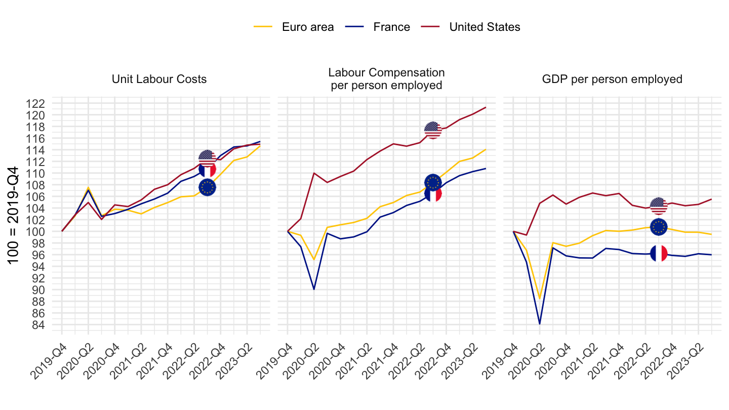
2000-
Code
ULC_EEQ %>%
  filter(MEASURE == "IXOBSA",
         SUBJECT == "ULQELP01",
         LOCATION %in% c("EA19", "USA", "FRA"),
         FREQUENCY == "Q") %>%
  left_join(ULC_EEQ_var$LOCATION, by = "LOCATION") %>%
  quarter_to_date %>%
  filter(year(date) >= 2008) %>%
  group_by(Location) %>%
  mutate(obsValue = 100*obsValue/obsValue[date == as.Date("2008-01-01")]) %>%
  mutate(Location = ifelse(LOCATION == "EA19", "Europe", Location)) %>%
  left_join(colors, by = c("Location" = "country")) %>%
  mutate(color = color2) %>%
  ggplot() + geom_line(aes(x = date, y = obsValue, color = color)) +

  theme_minimal() + ylab("GDP Per person employed") + xlab("") + add_3flags +
  scale_x_date(breaks = seq(1920, 2100, 1) %>% paste0("-01-01") %>% as.Date,
               labels = date_format("%Y")) +
  scale_color_identity() +
  theme(legend.position = c(0.8, 0.2),
        legend.title = element_blank()) +
  scale_y_continuous(breaks = seq(0, 200, 5))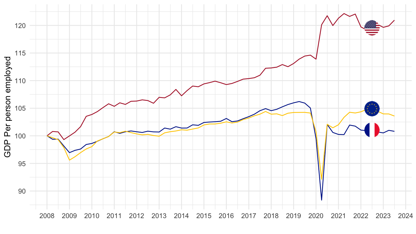
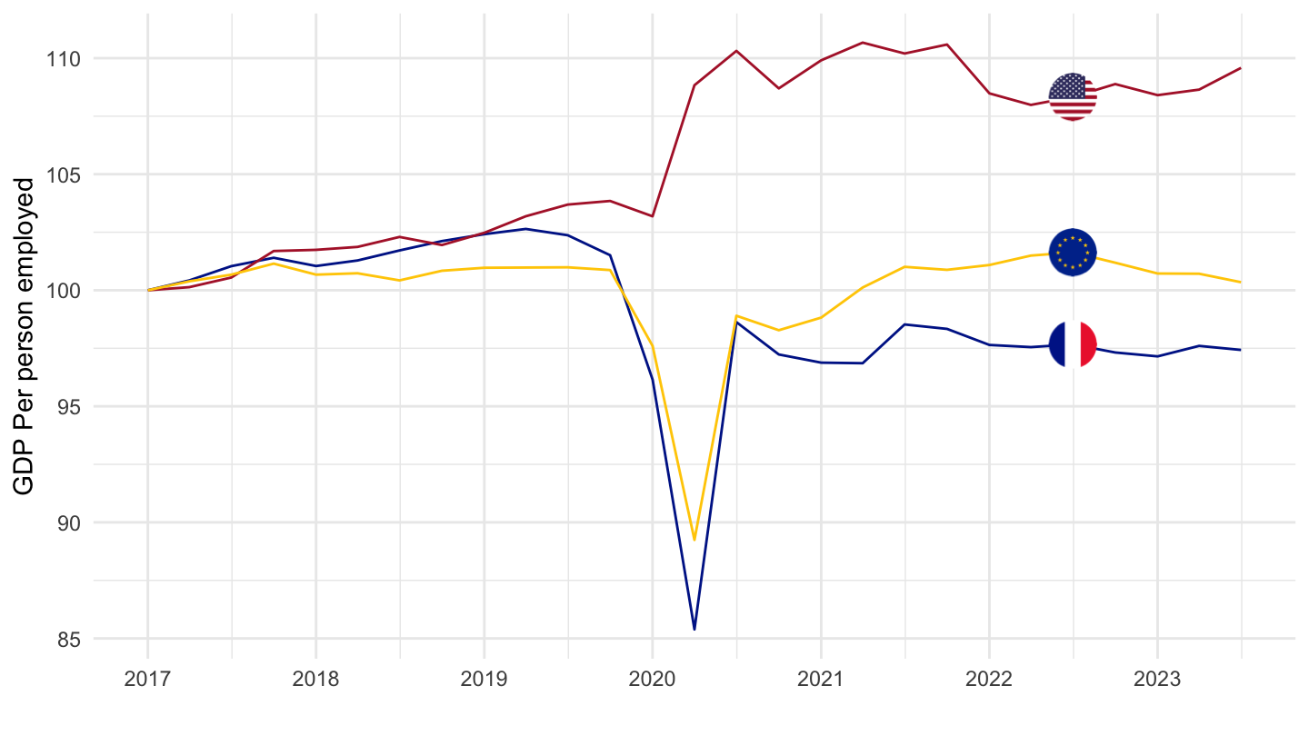
2017-
Code
ULC_EEQ %>%
  filter(MEASURE == "IXOBSA",
         SUBJECT == "ULQELP01",
         LOCATION %in% c("EA19", "USA", "FRA"),
         FREQUENCY == "Q") %>%
  left_join(ULC_EEQ_var$LOCATION, by = "LOCATION") %>%
  quarter_to_date %>%
  filter(year(date) >= 2017) %>%
  group_by(Location) %>%
  mutate(obsValue = 100*obsValue/obsValue[date == as.Date("2017-01-01")]) %>%
  mutate(Location = ifelse(LOCATION == "EA19", "Europe", Location)) %>%
  left_join(colors, by = c("Location" = "country")) %>%
  mutate(color = color2) %>%
  ggplot() + geom_line(aes(x = date, y = obsValue, color = color)) +

  theme_minimal() + ylab("GDP Per person employed") + xlab("") + add_3flags +
  scale_x_date(breaks = seq(1920, 2100, 1) %>% paste0("-01-01") %>% as.Date,
               labels = date_format("%Y")) +
  scale_color_identity() +
  theme(legend.position = c(0.8, 0.2),
        legend.title = element_blank()) +
  scale_y_continuous(breaks = seq(0, 200, 5))