Labour cost levels by NACE Rev. 2 activity
Data - Eurostat
Info
Last observation: Annual: 2025 (N = 10,286)
First observation: Annual: 2008 (N = 6,080)
Last data update: 23 jul 2026, 22:14. Last compile: 24 jul 2026, 02:10
Structure
Individual countries
France
2020
Code
lc_lci_lev %>%
  filter(time == "2020",
         unit == "EUR",
         geo %in% c("FR"),
         lcstruct != "D2-D4_MD5_RAT") %>%

  select(Lcstruct, nace_r2, values) %>%

  spread(Lcstruct, values) %>%
  arrange(-`Labour cost for LCI (compensation of employees plus taxes minus subsidies)`) %>%
  {if (is_html_output()) datatable(., filter = 'top', rownames = F, escape = F) else .}
2019
Code
lc_lci_lev %>%
  filter(time == "2019",
         unit == "EUR",
         geo %in% c("FR"),
         lcstruct != "D2-D4_MD5_RAT") %>%

  select(Lcstruct, nace_r2, values) %>%

  spread(Lcstruct, values) %>%
  {if (is_html_output()) datatable(., filter = 'top', rownames = F, escape = F) else .}
Germany
2020
Code
lc_lci_lev %>%
  filter(time == "2020",
         unit == "EUR",
         geo %in% c("DE"),
         lcstruct != "D2-D4_MD5_RAT") %>%

  select(Lcstruct, nace_r2, values) %>%

  spread(Lcstruct, values) %>%
  {if (is_html_output()) datatable(., filter = 'top', rownames = F, escape = F) else .}
2019
Code
lc_lci_lev %>%
  filter(time == "2019",
         unit == "EUR",
         geo %in% c("DE"),
         lcstruct != "D2-D4_MD5_RAT") %>%

  select(Lcstruct, nace_r2, values) %>%

  spread(Lcstruct, values) %>%
  {if (is_html_output()) datatable(., filter = 'top', rownames = F, escape = F) else .}
France VS Germany
B-E - Industry (except construction)
France, Germany
All
Code
load_data("eurostat/nace_r2_fr.RData")
lc_lci_lev %>%
  filter(geo %in% c("FR", "DE"),
         # SCPOLDPEN: Old age pension
         lcstruct == "D1_D4_MD5",
         # TOTAL: Total
         nace_r2 %in% c("B-E", "B-N", "C"),
         unit == "EUR") %>%
  year_to_date %>%


  left_join(colors, by = c("Geo" = "country")) %>%
  ggplot + theme_minimal() + geom_line(aes(x = date, y = values, color = color, linetype = Nace_r2)) +
  xlab("") + ylab("Coût horaire du travail") + add_4flags + scale_color_identity() +
  scale_linetype_manual(values = c("dashed", "solid", "dotted")) +
  scale_x_date(breaks = as.Date(paste0(seq(1960, 2100, 1), "-01-01")),
               labels = date_format("%Y")) +
  theme(legend.position = c(0.2, 0.8),
        legend.title = element_blank()) +
  scale_y_continuous(breaks = seq(0, 60, 1),
                     labels = scales::dollar_format(su = "€", p = ""))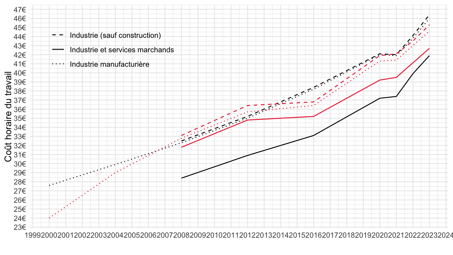
2009-
Code
load_data("eurostat/nace_r2_fr.RData")
lc_lci_lev %>%
  filter(geo %in% c("FR", "DE"),
         # SCPOLDPEN: Old age pension
         lcstruct == "D1_D4_MD5",
         # TOTAL: Total
         nace_r2 %in% c("C", "B-N"),
         unit == "EUR") %>%
  year_to_date %>%
  filter(date >= as.Date("2008-01-01")) %>%


  left_join(colors, by = c("Geo" = "country")) %>%
  ggplot + theme_minimal() + geom_line(aes(x = date, y = values, color = color, linetype = Nace_r2)) +
  xlab("") + ylab("Coût horaire du travail") + add_4flags + scale_color_identity() +
  scale_linetype_manual(values = c("dashed", "solid")) +
  scale_x_date(breaks = as.Date(paste0(seq(1960, 2100, 1), "-01-01")),
               labels = date_format("%Y")) +
  theme(legend.position = c(0.2, 0.8),
        legend.title = element_blank()) +
  scale_y_continuous(breaks = seq(0, 60, 1),
                     labels = scales::dollar_format(su = "€", p = ""))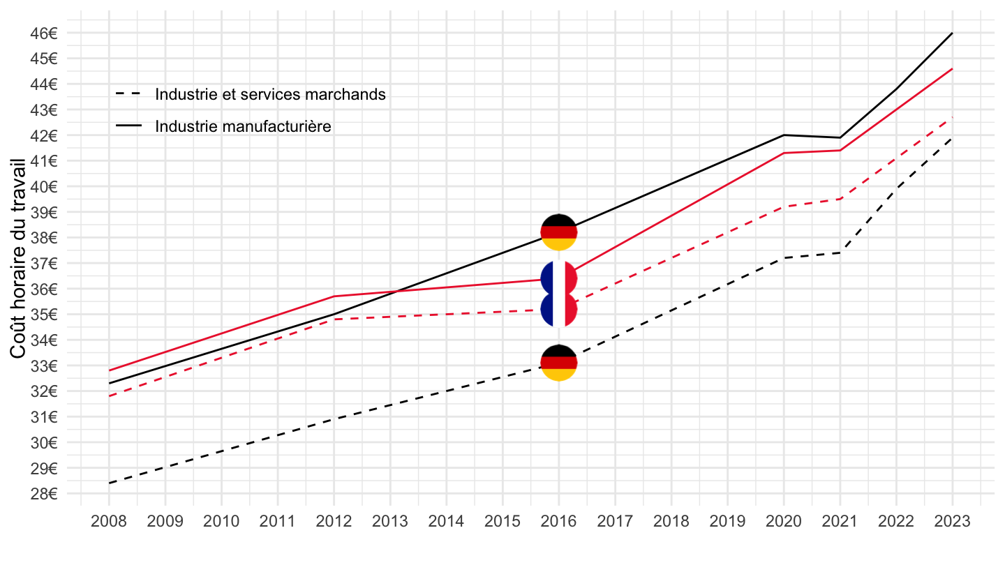
D1_D4_MD5 - Labour cost for LCI (compensation of employees plus taxes minus subsidies)
France, Germany, Italy, Spain
Code
lc_lci_lev %>%
  filter(lcstruct == "D1_D4_MD5",
         time == "2019",
         unit == "EUR",
         geo %in% c("FR", "DE", "IT", "ES")) %>%

  mutate(Geo = ifelse(geo == "DE", "Germany", Geo)) %>%
  mutate(Geo = gsub(" ", "-", str_to_lower(Geo)),
         Geo = paste0('<img src="../../bib/flags/vsmall/', Geo, '.png" alt="Flag">')) %>%
  select(nace_r2, Geo, values) %>%

  spread(Geo, values) %>%
  {if (is_html_output()) datatable(., filter = 'top', rownames = F, escape = F) else .}
B - Mining
Code
lc_lci_lev %>%
  filter(geo %in% c("FR", "DE", "IT"),
         # SCPOLDPEN: Old age pension
         lcstruct == "D1_D4_MD5",
         # TOTAL: Total
         nace_r2 == "B",
         unit == "EUR") %>%
  year_to_date %>%

  left_join(colors, by = c("Geo" = "country")) %>%
  ggplot + theme_minimal() + geom_line(aes(x = date, y = values, color = color)) +
  xlab("") + ylab("Hourly wages + taxes - subsidies (Industry)") + add_3flags + scale_color_identity() +
  scale_x_date(breaks = as.Date(paste0(seq(1960, 2100, 2), "-01-01")),
               labels = date_format("%Y")) +
  theme(legend.position = "none") +
  scale_y_continuous(breaks = seq(0, 60, 1),
                     labels = scales::dollar_format(su = "€", p = ""))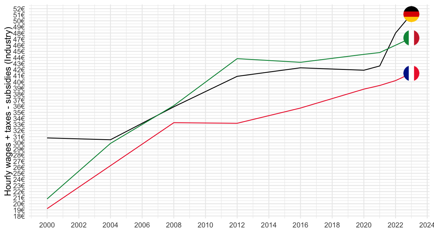
B-E - Industry (except construction)
France, Italy, Spain
Code
lc_lci_lev %>%
  filter(geo %in% c("FR", "ES", "IT"),
         # SCPOLDPEN: Old age pension
         lcstruct == "D1_D4_MD5",
         # TOTAL: Total
         nace_r2 == "B-E",
         unit == "EUR") %>%
  year_to_date %>%

  left_join(colors, by = c("Geo" = "country")) %>%
  ggplot + theme_minimal() + geom_line(aes(x = date, y = values, color = color)) +
  xlab("") + ylab("Hourly wages + taxes - subsidies (Industry)") + add_3flags + scale_color_identity() +
  scale_x_date(breaks = as.Date(paste0(seq(1960, 2100, 2), "-01-01")),
               labels = date_format("%Y")) +
  theme(legend.position = "none") +
  scale_y_continuous(breaks = seq(0, 60, 1),
                     labels = scales::dollar_format(su = "€", p = ""))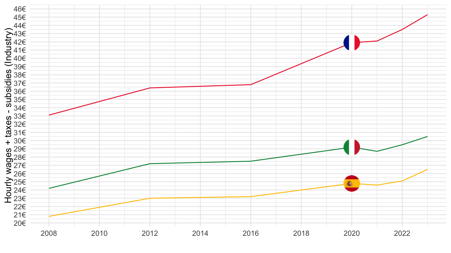
France, Germany, Italy
Code
lc_lci_lev %>%
  filter(geo %in% c("FR", "DE", "IT"),
         # SCPOLDPEN: Old age pension
         lcstruct == "D1_D4_MD5",
         # TOTAL: Total
         nace_r2 == "B-E",
         unit == "EUR") %>%
  year_to_date %>%

  left_join(colors, by = c("Geo" = "country")) %>%
  ggplot + theme_minimal() + geom_line(aes(x = date, y = values, color = color)) +
  xlab("") + ylab("Hourly wages + taxes - subsidies (Industry)") + add_3flags + scale_color_identity() +
  scale_x_date(breaks = as.Date(paste0(seq(1960, 2100, 2), "-01-01")),
               labels = date_format("%Y")) +
  theme(legend.position = "none") +
  scale_y_continuous(breaks = seq(0, 60, 1),
                     labels = scales::dollar_format(su = "€", p = ""))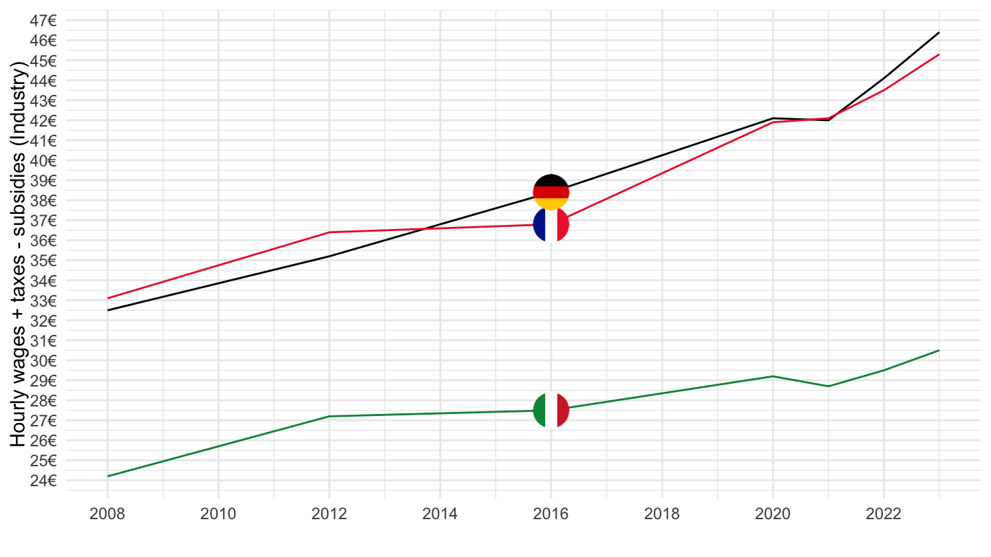
Greece, Portugal, Spain
Code
lc_lci_lev %>%
  filter(geo %in% c("EL", "PT", "ES"),
         # SCPOLDPEN: Old age pension
         lcstruct == "D1_D4_MD5",
         # TOTAL: Total
         nace_r2 == "B-E",
         unit == "EUR") %>%
  year_to_date %>%

  left_join(colors, by = c("Geo" = "country")) %>%
  ggplot + theme_minimal() + geom_line(aes(x = date, y = values, color = color)) +
  xlab("") + ylab("Hourly wages + taxes - subsidies (Industry)") + add_3flags + scale_color_identity() +
  scale_x_date(breaks = as.Date(paste0(seq(1960, 2100, 2), "-01-01")),
               labels = date_format("%Y")) +
  theme(legend.position = "none") +
  scale_y_continuous(breaks = seq(0, 60, 1),
                     labels = scales::dollar_format(su = "€", p = ""))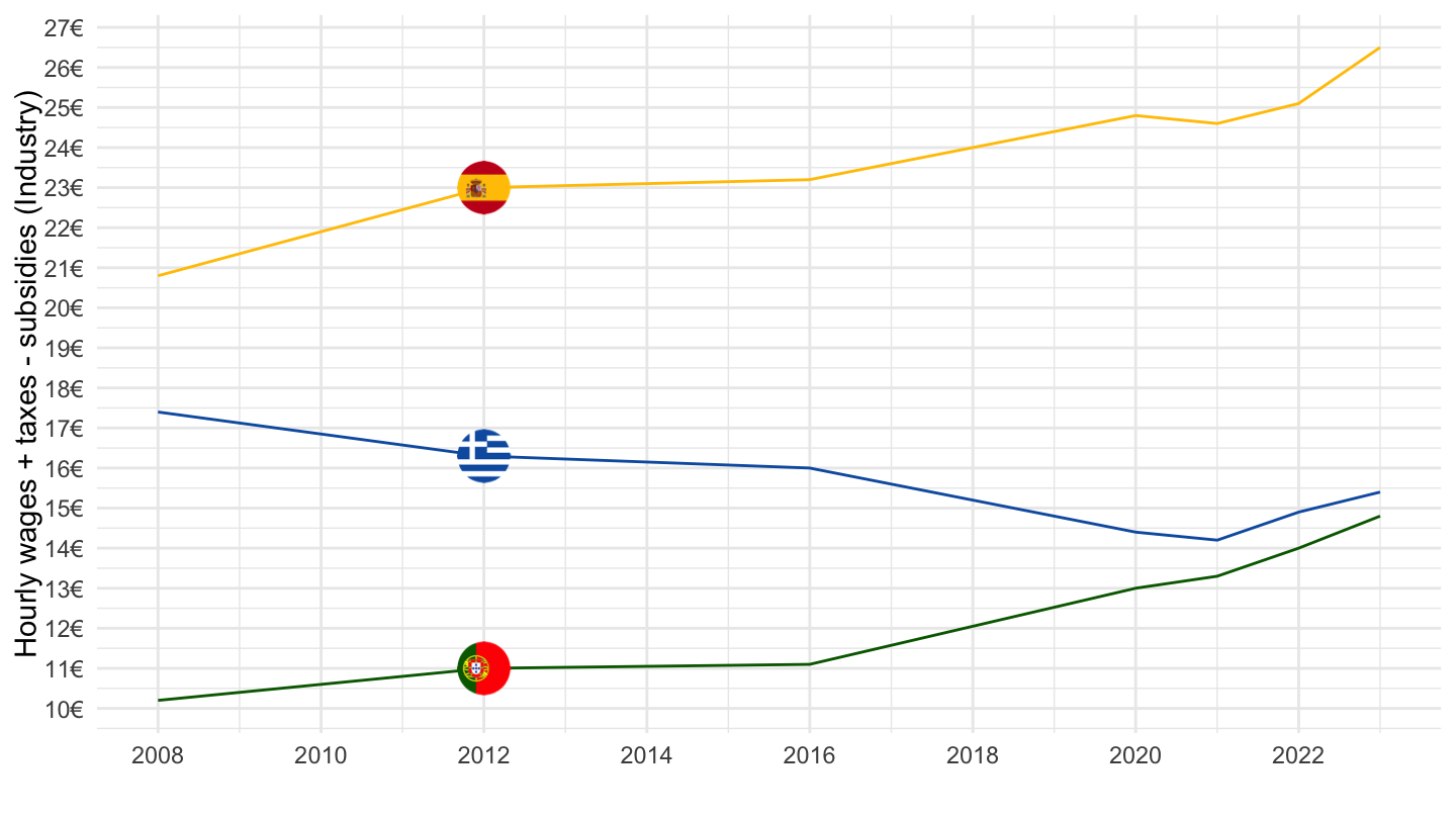
C - Manufacturing
Code
lc_lci_lev %>%
  filter(geo %in% c("FR", "DE", "IT"),
         # SCPOLDPEN: Old age pension
         lcstruct == "D1_D4_MD5",
         # TOTAL: Total
         nace_r2 == "C",
         unit == "EUR") %>%
  year_to_date %>%

  left_join(colors, by = c("Geo" = "country")) %>%
  ggplot + theme_minimal() + geom_line(aes(x = date, y = values, color = color)) +
  xlab("") + ylab("Hourly wages + taxes - subsidies (Manufacturing)") + add_3flags + scale_color_identity() +
  scale_x_date(breaks = as.Date(paste0(seq(1960, 2100, 2), "-01-01")),
               labels = date_format("%Y")) +
  theme(legend.position = "none") +
  scale_y_continuous(breaks = seq(0, 60, 1),
                     labels = scales::dollar_format(su = "€", p = ""))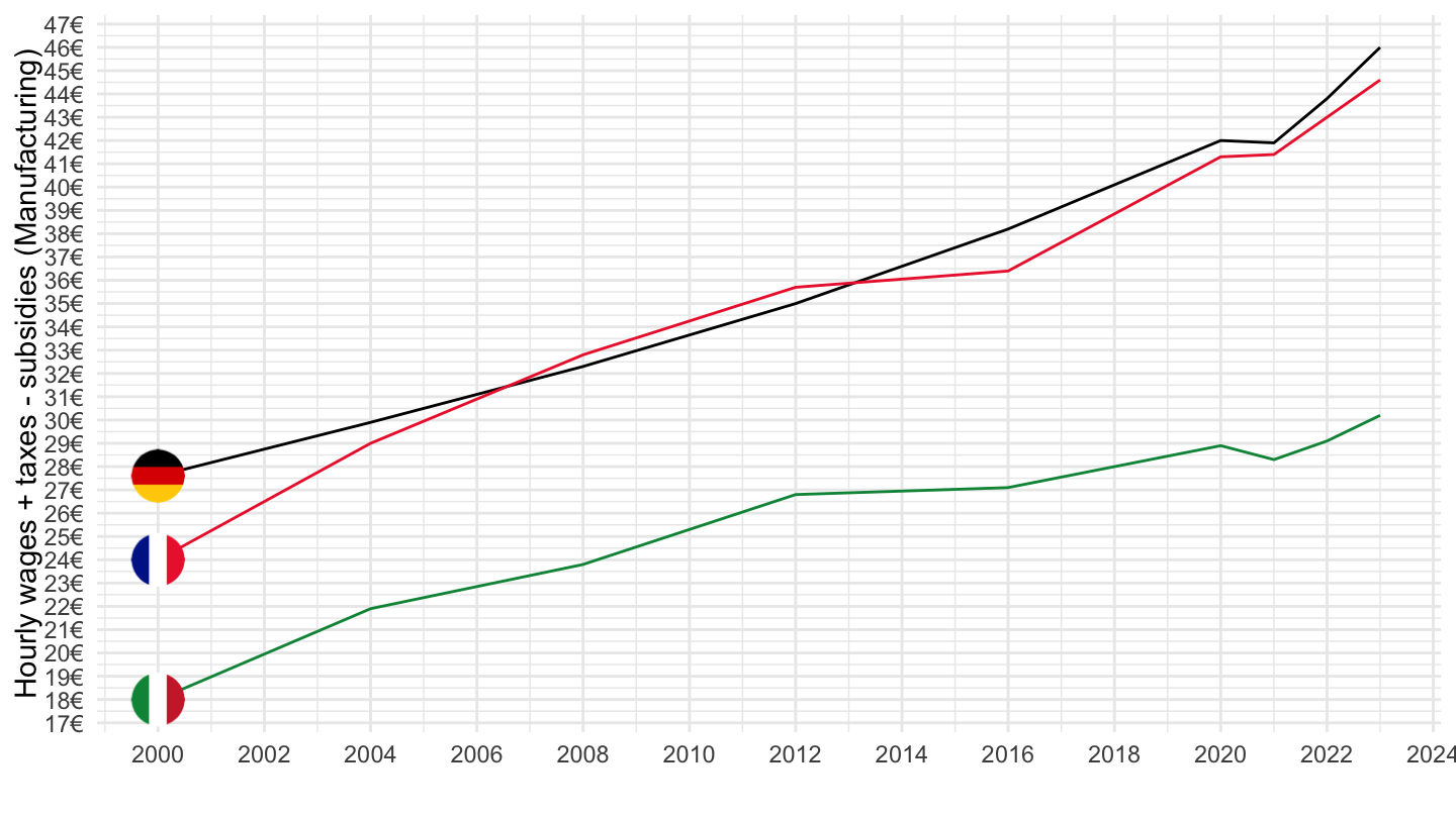
D11 - Wages and salaries (total)
France, Germany, Italy, Spain
Code
lc_lci_lev %>%
  filter(lcstruct == "D11",
         time == "2019",
         unit == "EUR",
         geo %in% c("FR", "DE", "IT", "ES")) %>%

  mutate(Geo = ifelse(geo == "DE", "Germany", Geo)) %>%
  mutate(Geo = gsub(" ", "-", str_to_lower(Geo)),
         Geo = paste0('<img src="../../bib/flags/vsmall/', Geo, '.png" alt="Flag">')) %>%
  select(nace_r2, Geo, values) %>%

  spread(Geo, values) %>%
  {if (is_html_output()) datatable(., filter = 'top', rownames = F, escape = F) else .}
Greece, Portugal, Spain
Code
lc_lci_lev %>%
  filter(lcstruct == "D11",
         time == "2019",
         unit == "EUR",
         geo %in% c("EL", "ES", "PT")) %>%

  mutate(Geo = gsub(" ", "-", str_to_lower(Geo)),
         Geo = paste0('<img src="../../bib/flags/vsmall/', Geo, '.png" alt="Flag">')) %>%
  select(nace_r2, Geo, values) %>%

  spread(Geo, values) %>%
  {if (is_html_output()) datatable(., filter = 'top', rownames = F, escape = F) else .}
B-N - Business economy
France, Germany, Italy
Code
lc_lci_lev %>%
  filter(geo %in% c("FR", "DE", "IT"),
         # SCPOLDPEN: Old age pension
         lcstruct == "D11",
         # TOTAL: Total
         nace_r2 == "B-N",
         unit == "EUR") %>%
  year_to_date %>%

  left_join(colors, by = c("Geo" = "country")) %>%
  ggplot + theme_minimal() + geom_line(aes(x = date, y = values, color = color)) +
  xlab("") + ylab("Hourly Wage") + add_3flags + scale_color_identity() +
  scale_x_date(breaks = as.Date(paste0(seq(1960, 2100, 2), "-01-01")),
               labels = date_format("%Y")) +
  theme(legend.position = "none") +
  scale_y_continuous(breaks = seq(0, 60, 1),
                     labels = scales::dollar_format(su = "€", p = ""))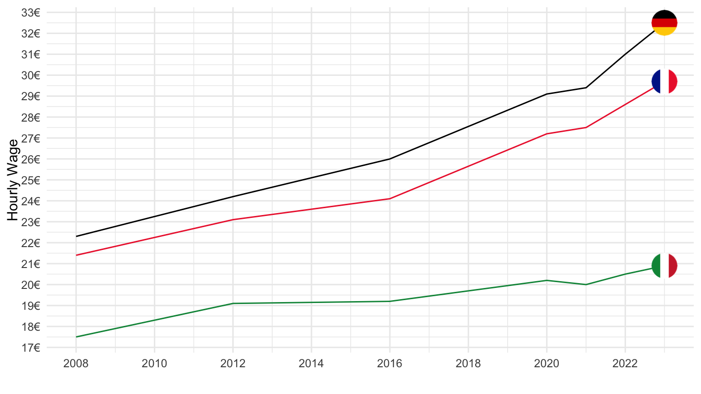
Greece, Portugal, Spain
Code
lc_lci_lev %>%
  filter(geo %in% c("EL", "ES", "PT"),
         # SCPOLDPEN: Old age pension
         lcstruct == "D11",
         # TOTAL: Total
         nace_r2 == "B-N",
         unit == "EUR") %>%
  year_to_date %>%

  left_join(colors, by = c("Geo" = "country")) %>%
  ggplot + theme_minimal() + geom_line(aes(x = date, y = values, color = color)) +
  xlab("") + ylab("Hourly Wage") + add_3flags + scale_color_identity() +
  scale_x_date(breaks = as.Date(paste0(seq(1960, 2100, 2), "-01-01")),
               labels = date_format("%Y")) +
  theme(legend.position = "none") +
  scale_y_continuous(breaks = seq(0, 60, 1),
                     labels = scales::dollar_format(su = "€", p = ""))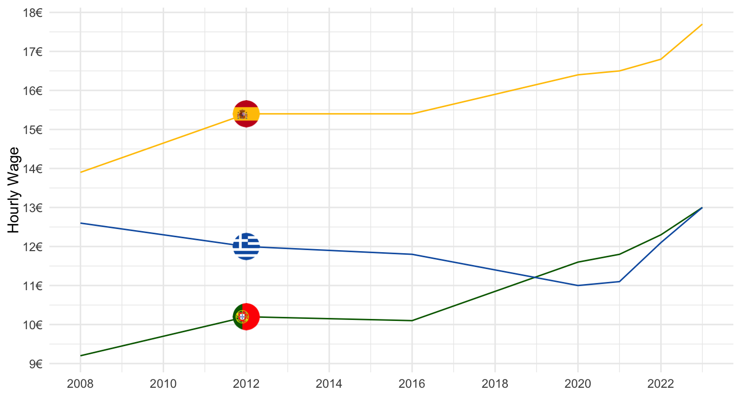
B - Mining
Code
lc_lci_lev %>%
  filter(geo %in% c("FR", "DE", "IT"),
         # SCPOLDPEN: Old age pension
         lcstruct == "D11",
         # TOTAL: Total
         nace_r2 == "B",
         unit == "EUR") %>%
  year_to_date %>%

  left_join(colors, by = c("Geo" = "country")) %>%
  ggplot + theme_minimal() + geom_line(aes(x = date, y = values, color = color)) +
  xlab("") + ylab("Hourly Wage") + add_3flags + scale_color_identity() +
  scale_x_date(breaks = as.Date(paste0(seq(1960, 2100, 2), "-01-01")),
               labels = date_format("%Y")) +
  theme(legend.position = "none") +
  scale_y_continuous(breaks = seq(0, 60, 1),
                     labels = scales::dollar_format(su = "€", p = ""))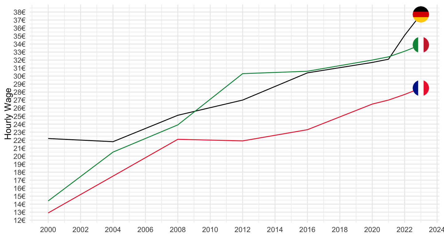
B-E - Industry (except construction)
English
Code
lc_lci_lev %>%
  filter(geo %in% c("FR", "DE", "IT"),
         # SCPOLDPEN: Old age pension
         lcstruct == "D11",
         # TOTAL: Total
         nace_r2 == "B-E",
         unit == "EUR") %>%
  year_to_date %>%

  left_join(colors, by = c("Geo" = "country")) %>%
  ggplot + theme_minimal() + geom_line(aes(x = date, y = values, color = color)) +
  xlab("") + ylab("Hourly Wage") + add_3flags + scale_color_identity() +
  scale_x_date(breaks = as.Date(paste0(seq(1960, 2100, 2), "-01-01")),
               labels = date_format("%Y")) +
  theme(legend.position = "none") +
  scale_y_continuous(breaks = seq(0, 60, 1),
                     labels = scales::dollar_format(su = "€", p = ""))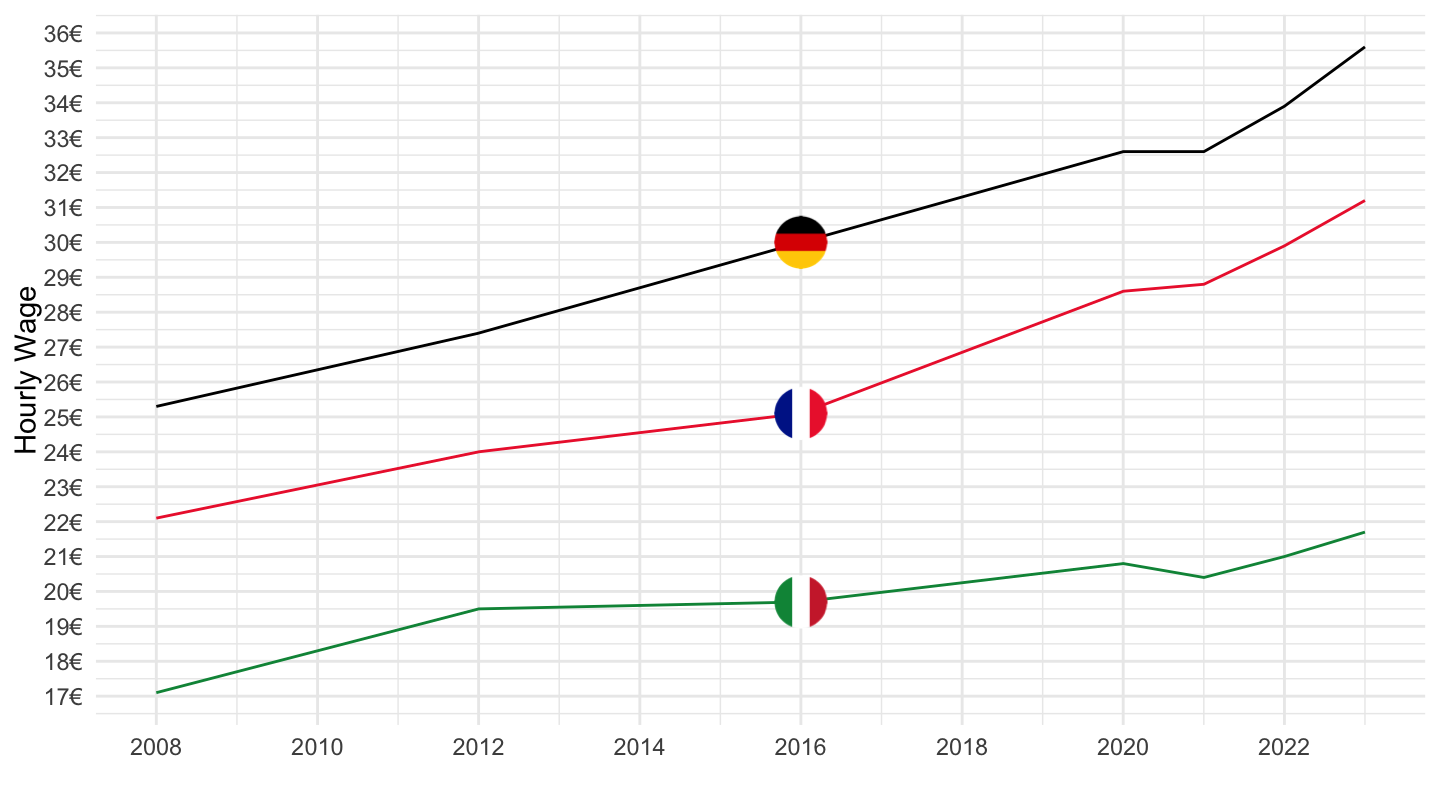
French
Code
lc_lci_lev %>%
  filter(geo %in% c("FR", "DE", "IT"),
         # SCPOLDPEN: Old age pension
         lcstruct == "D11",
         # TOTAL: Total
         nace_r2 == "B-E",
         unit == "EUR") %>%
  year_to_date %>%

  left_join(colors, by = c("Geo" = "country")) %>%
  ggplot + theme_minimal() + geom_line(aes(x = date, y = values, color = color)) +
  xlab("") + ylab("Hourly Wage") + add_3flags + scale_color_identity() +
  scale_x_date(breaks = as.Date(paste0(seq(1960, 2100, 2), "-01-01")),
               labels = date_format("%Y")) +
  theme(legend.position = "none") +
  scale_y_continuous(breaks = seq(0, 60, 1),
                     labels = scales::dollar_format(su = "€", p = ""))
C - Manufacturing
English
Code
lc_lci_lev %>%
  filter(geo %in% c("FR", "DE", "IT"),
         # SCPOLDPEN: Old age pension
         lcstruct == "D11",
         # TOTAL: Total
         nace_r2 == "C",
         unit == "EUR") %>%
  year_to_date %>%

  left_join(colors, by = c("Geo" = "country")) %>%
  ggplot + theme_minimal() + geom_line(aes(x = date, y = values, color = color)) +
  xlab("") + ylab("Hourly Wage") + add_3flags + scale_color_identity() +
  scale_x_date(breaks = as.Date(paste0(seq(1960, 2100, 2), "-01-01")),
               labels = date_format("%Y")) +
  theme(legend.position = "none") +
  scale_y_continuous(breaks = seq(0, 60, 1),
                     labels = scales::dollar_format(su = "€", p = ""))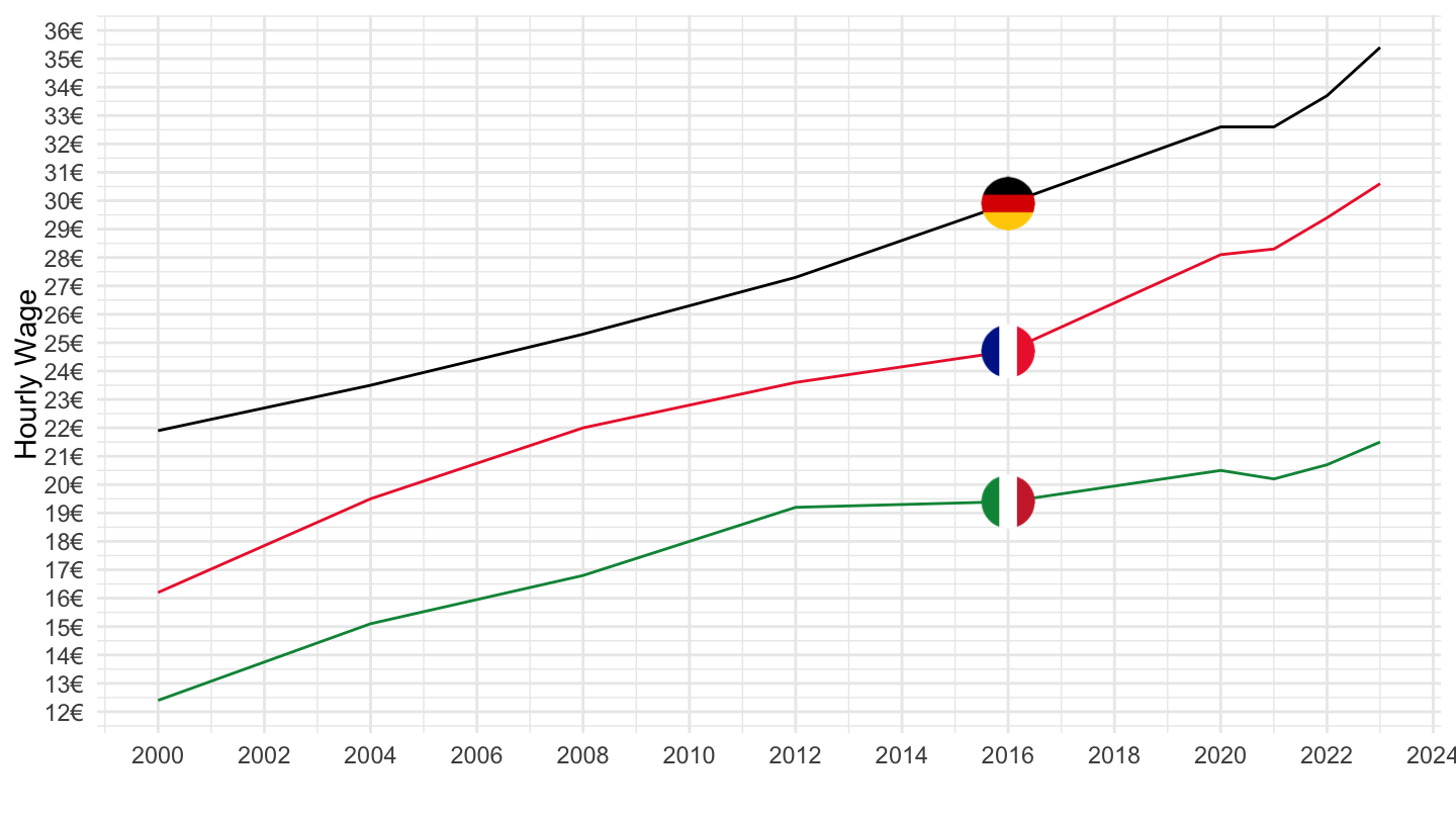
French
Code
lc_lci_lev %>%
  filter(geo %in% c("FR", "DE", "IT"),
         # SCPOLDPEN: Old age pension
         lcstruct == "D11",
         # TOTAL: Total
         nace_r2 == "C",
         unit == "EUR") %>%
  year_to_date %>%

  left_join(colors, by = c("Geo" = "country")) %>%
  ggplot + theme_minimal() + geom_line(aes(x = date, y = values, color = color)) +
  xlab("") + ylab("Salaire Horaire") + add_3flags + scale_color_identity() +
  scale_x_date(breaks = as.Date(paste0(seq(1960, 2100, 2), "-01-01")),
               labels = date_format("%Y")) +
  theme(legend.position = "none") +
  scale_y_continuous(breaks = seq(0, 60, 1),
                     labels = scales::dollar_format(su = "€", p = ""))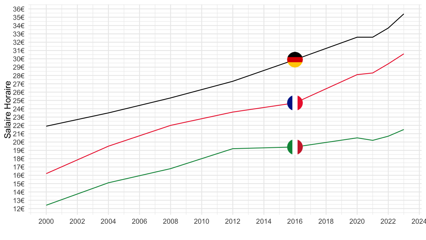
D12_D4_MD5 - Labour Costs Other than Wages and Salaries
France, Germany, Italy, Spain
Code
lc_lci_lev %>%
  filter(lcstruct == "D12_D4_MD5",
         time == "2019",
         unit == "EUR",
         geo %in% c("FR", "DE", "IT", "ES")) %>%

  mutate(Geo = ifelse(geo == "DE", "Germany", Geo)) %>%
  mutate(Geo = gsub(" ", "-", str_to_lower(Geo)),
         Geo = paste0('<img src="../../bib/flags/vsmall/', Geo, '.png" alt="Flag">')) %>%
  select(nace_r2, Geo, values) %>%

  spread(Geo, values) %>%
  {if (is_html_output()) datatable(., filter = 'top', rownames = F, escape = F) else .}
B - Mining
Code
lc_lci_lev %>%
  filter(geo %in% c("FR", "DE", "IT"),
         # SCPOLDPEN: Old age pension
         lcstruct == "D12_D4_MD5",
         # TOTAL: Total
         nace_r2 == "B",
         unit == "EUR") %>%
  year_to_date %>%

  ggplot + theme_minimal() + geom_line(aes(x = date, y = values, color = Geo)) +
  xlab("") + ylab("Labour Costs Other than Wages and Salaries") +
  scale_color_manual(values = c("#002395", "#000000", "#009246")) +
  add_3flags +
  scale_x_date(breaks = as.Date(paste0(seq(1960, 2100, 2), "-01-01")),
               labels = date_format("%Y")) +
  theme(legend.position = "none") +
  scale_y_continuous(breaks = seq(0, 60, 1),
                     labels = scales::dollar_format(su = "€", p = ""))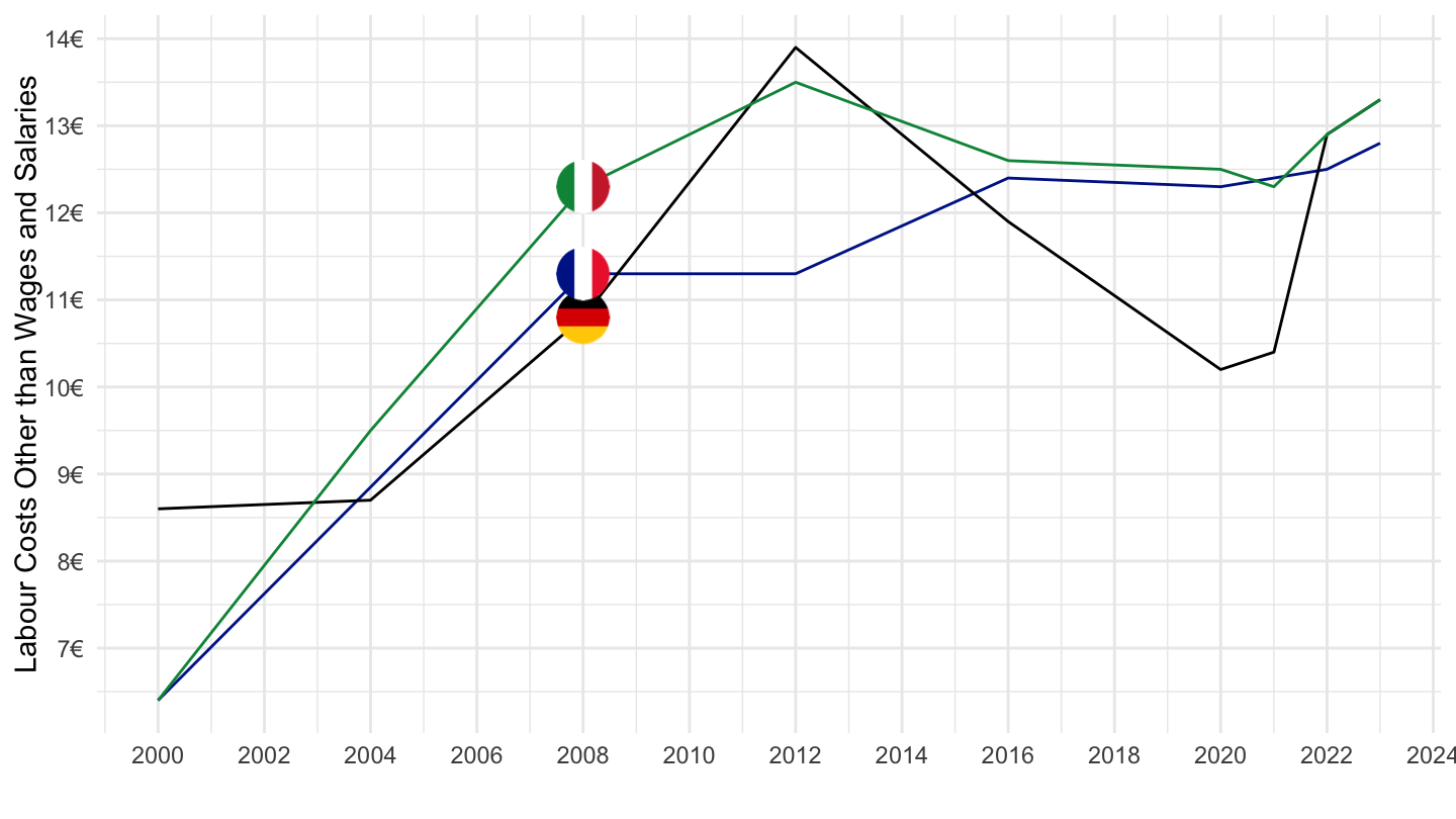
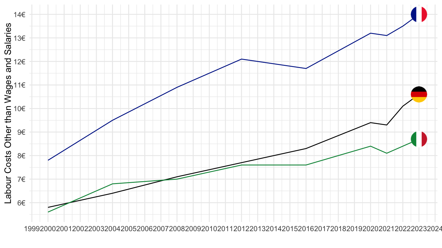
B-E - Industry (except construction)
Code
lc_lci_lev %>%
  filter(geo %in% c("FR", "DE", "IT"),
         # SCPOLDPEN: Old age pension
         lcstruct == "D12_D4_MD5",
         # TOTAL: Total
         nace_r2 == "B-E",
         unit == "EUR") %>%
  year_to_date %>%

  ggplot + theme_minimal() + geom_line(aes(x = date, y = values, color = Geo)) +
  xlab("") + ylab("Labour Costs Other than Wages and Salaries") +
  scale_color_manual(values = c("#002395", "#000000", "#009246")) +
  add_3flags +
  scale_x_date(breaks = as.Date(paste0(seq(1960, 2100, 1), "-01-01")),
               labels = date_format("%Y")) +
  theme(legend.position = "none") +
  scale_y_continuous(breaks = seq(0, 60, 1),
                     labels = scales::dollar_format(su = "€", p = ""))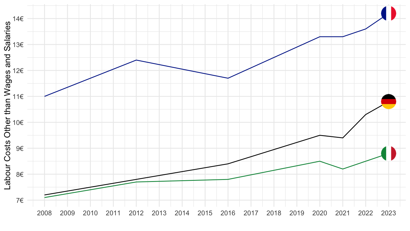
C - Manufacturing
Code
lc_lci_lev %>%
  filter(geo %in% c("FR", "DE", "IT"),
         # SCPOLDPEN: Old age pension
         lcstruct == "D12_D4_MD5",
         # TOTAL: Total
         nace_r2 == "C",
         unit == "EUR") %>%
  year_to_date %>%

  ggplot + theme_minimal() + geom_line(aes(x = date, y = values, color = Geo)) +
  xlab("") + ylab("Labour Costs Other than Wages and Salaries") +
  scale_color_manual(values = c("#002395", "#000000", "#009246")) +
  add_3flags +
  scale_x_date(breaks = as.Date(paste0(seq(1960, 2100, 1), "-01-01")),
               labels = date_format("%Y")) +
  theme(legend.position = "none") +
  scale_y_continuous(breaks = seq(0, 60, 1),
                     labels = scales::dollar_format(su = "€", p = ""))