| source | dataset | Title | .html | .rData |
|---|---|---|---|---|
| oecd | EAR_MEI | Hourly Earnings (MEI) | 2026-07-23 | 2024-04-16 |
| oecd | PRICES_CPI | Consumer price indices (CPIs) | 2024-04-16 | 2024-04-15 |
Hourly Earnings (MEI)
Data - OECD
Info
Data on wages
Code
load_data("wages.RData")
wages %>%
source_dataset_file_updates()| source | dataset | Title | .html | .rData |
|---|---|---|---|---|
| eurostat | earn_mw_cur | Monthly minimum wages - bi-annual data | 2026-07-23 | 2026-07-23 |
| eurostat | ei_lmlc_q | Labour cost index, nominal value - quarterly data | 2026-07-23 | 2026-07-23 |
| eurostat | lc_lci_lev | Labour cost levels by NACE Rev. 2 activity | 2026-07-23 | 2026-07-23 |
| eurostat | lc_lci_r2_q | Labour cost index by NACE Rev. 2 activity - nominal value, quarterly data | 2026-07-23 | 2026-07-23 |
| eurostat | nama_10_lp_ulc | Labour productivity and unit labour costs | 2026-07-22 | 2026-07-23 |
| eurostat | namq_10_lp_ulc | Labour productivity and unit labour costs | 2026-07-23 | 2026-07-23 |
| eurostat | tps00155 | Minimum wages | 2026-07-23 | 2026-07-23 |
| fred | wage | Wage | 2026-07-22 | 2026-07-22 |
| ilo | EAR_4MTH_SEX_ECO_CUR_NB_A | Mean nominal monthly earnings of employees by sex and economic activity -- Harmonized series | 2024-06-20 | 2023-06-01 |
| ilo | EAR_XEES_SEX_ECO_NB_Q | Mean nominal monthly earnings of employees by sex and economic activity -- Harmonized series | 2024-06-20 | 2023-06-01 |
| oecd | AV_AN_WAGE | Average annual wages | 2026-07-23 | 2026-07-23 |
| oecd | AWCOMP | Taxing Wages - Comparative tables | 2026-07-23 | 2023-09-09 |
| oecd | EAR_MEI | Hourly Earnings (MEI) | 2026-07-23 | 2024-04-16 |
| oecd | HH_DASH | Household Dashboard | 2026-07-23 | 2023-09-09 |
| oecd | MIN2AVE | Minimum relative to average wages of full-time workers - MIN2AVE | 2026-02-22 | 2023-09-09 |
| oecd | RMW | Real Minimum Wages - RMW | 2026-07-23 | 2024-03-12 |
| oecd | ULC_EEQ | Unit labour costs and labour productivity (employment based), Total economy | 2026-07-23 | 2024-04-15 |
Last
| obsTime | FREQUENCY | Nobs |
|---|---|---|
| 2022 | A | 93 |
| 2021 | A | 95 |
| 2020 | A | 93 |
| 2023-11 | M | 5 |
| 2023-10 | M | 14 |
| 2023-09 | M | 32 |
| 2023-Q3 | Q | 71 |
| 2023-Q2 | Q | 86 |
| 2023-Q1 | Q | 91 |
Detail
The Hourly Earnings (MEI) dataset contains predominantly monthly statistics, and associated statistical methodological information, for the 38 OECD member countries and for selected non-member economies.
The MEI Earnings dataset provides monthly and quarterly data on employees’ earnings series. It includes earnings series in manufacturing and for the private economic sector. Mostly the sources of the data are business surveys covering different economic sectors, but in some cases administrative data are also used. The target series for hourly earnings correspond to seasonally adjusted average total earnings paid per employed person per hour, including overtime pay and regularly recurring cash supplements. Where hourly earnings series are not available, a series could refer to weekly or monthly earnings. In this case, a series for full-time or full-time equivalent employees is preferred to an all employees series.
SUBJECT
Code
EAR_MEI %>%
  left_join(EAR_MEI_var$SUBJECT, by = "SUBJECT") %>%
  group_by(SUBJECT, Subject) %>%
  summarise(nobs = n()) %>%
  arrange(-nobs) %>%
print_table_conditional()| SUBJECT | Subject | nobs |
|---|---|---|
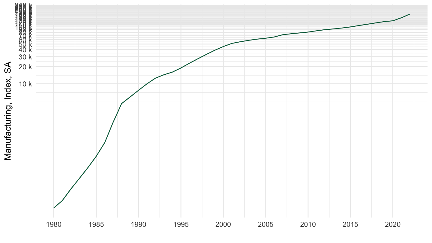
| LCEAMN01_IXOBSA | Manufacturing, Index, SA | 19040 |
| LCEAMN01_IXOB | Manufacturing, Index | 15978 |
| LCEAPR_IXOBSA | Private Sector, Index, SA | 6568 |
FREQUENCY
Code
EAR_MEI %>%
  left_join(EAR_MEI_var$FREQUENCY, by = "FREQUENCY") %>%
  group_by(FREQUENCY, Frequency) %>%
  summarise(nobs = n()) %>%
  arrange(-nobs) %>%
print_table_conditional()| FREQUENCY | Frequency | nobs |
|---|---|---|
| M | Monthly | 22249 |
| Q | Quarterly | 15555 |
| A | Annual | 3782 |
LOCATION
All
Code
EAR_MEI %>%
  left_join(EAR_MEI_var$LOCATION, by = "LOCATION") %>%
  group_by(LOCATION, Location) %>%
  summarise(Nobs = n()) %>%
  arrange(-Nobs) %>%
  mutate(Flag = gsub(" ", "-", str_to_lower(gsub(" ", "-", Location))),
         Flag = paste0('<img src="../../icon/flag/vsmall/', Flag, '.png" alt="Flag">')) %>%
  select(Flag, everything()) %>%
  {if (is_html_output()) datatable(., filter = 'top', rownames = F, escape = F) else .}
Location x Frequency
Code
EAR_MEI %>%
  left_join(EAR_MEI_var$LOCATION, by = "LOCATION") %>%
  group_by(LOCATION, Location, FREQUENCY) %>%
  summarise(Nobs = n()) %>%
  arrange(-Nobs) %>%
  mutate(Flag = gsub(" ", "-", str_to_lower(gsub(" ", "-", Location))),
         Flag = paste0('<img src="../../icon/flag/vsmall/', Flag, '.png" alt="Flag">')) %>%
  select(Flag, everything()) %>%
  {if (is_html_output()) datatable(., filter = 'top', rownames = F, escape = F) else .}
Annual
Code
EAR_MEI %>%
  filter(FREQUENCY == "A") %>%
  left_join(EAR_MEI_var$LOCATION, by = "LOCATION") %>%
  group_by(LOCATION, Location) %>%
  summarise(Nobs = n()) %>%
  arrange(-Nobs) %>%
  mutate(Flag = gsub(" ", "-", str_to_lower(gsub(" ", "-", Location))),
         Flag = paste0('<img src="../../icon/flag/vsmall/', Flag, '.png" alt="Flag">')) %>%
  select(Flag, everything()) %>%
  {if (is_html_output()) datatable(., filter = 'top', rownames = F, escape = F) else .}
Quarterly
Code
EAR_MEI %>%
  filter(FREQUENCY == "Q") %>%
  left_join(EAR_MEI_var$LOCATION, by = "LOCATION") %>%
  group_by(LOCATION, Location) %>%
  summarise(Nobs = n()) %>%
  arrange(-Nobs) %>%
  mutate(Flag = gsub(" ", "-", str_to_lower(gsub(" ", "-", Location))),
         Flag = paste0('<img src="../../icon/flag/vsmall/', Flag, '.png" alt="Flag">')) %>%
  select(Flag, everything()) %>%
  {if (is_html_output()) datatable(., filter = 'top', rownames = F, escape = F) else .}
Monthly
Code
EAR_MEI %>%
  filter(FREQUENCY == "M") %>%
  left_join(EAR_MEI_var$LOCATION, by = "LOCATION") %>%
  group_by(LOCATION, Location) %>%
  summarise(Nobs = n()) %>%
  arrange(-Nobs) %>%
  mutate(Flag = gsub(" ", "-", str_to_lower(gsub(" ", "-", Location))),
         Flag = paste0('<img src="../../icon/flag/vsmall/', Flag, '.png" alt="Flag">')) %>%
  select(Flag, everything()) %>%
  {if (is_html_output()) datatable(., filter = 'top', rownames = F, escape = F) else .}
obsTime
Code
EAR_MEI %>%
  group_by(obsTime) %>%
  summarise(Nobs = n()) %>%
  arrange(desc(obsTime)) %>%
  print_table_conditional()
Europe VS U.S.
LCEAMN01_IXOBSA - Manufacturing, Index, SA
Code
EAR_MEI %>%
  filter(SUBJECT == "LCEAMN01_IXOBSA",
         FREQUENCY == "Q",
         LOCATION %in% c("USA", "EA19")) %>%
  quarter_to_date %>%
  filter(date >= as.Date("2019-01-01")) %>%
  left_join(EAR_MEI_var$LOCATION, by = "LOCATION") %>%
  mutate(Location = ifelse(LOCATION == "EA19", "Europe", Location)) %>%
  left_join(colors, by = c("Location" = "country")) %>%
  mutate(color = ifelse(LOCATION == "USA", color2, color)) %>%
  group_by(Location) %>%
  arrange(date) %>%
  mutate(obsValue = 100*obsValue / obsValue[date == as.Date("2019-01-01")]) %>%
  ggplot(.) + geom_line(aes(x = date, y = obsValue, color = color)) +
  scale_color_identity() + theme_minimal() + add_2flags +
  scale_x_date(breaks = seq(1920, 2100, 1) %>% paste0("-01-01") %>% as.Date,
               labels = date_format("%Y")) +
  scale_y_log10(breaks = seq(10, 500, 5),
                     labels = scales::dollar_format(accuracy = 1, suffix = "", prefix = "")) +
  ylab("Manufacturing, Index, SA") + xlab("")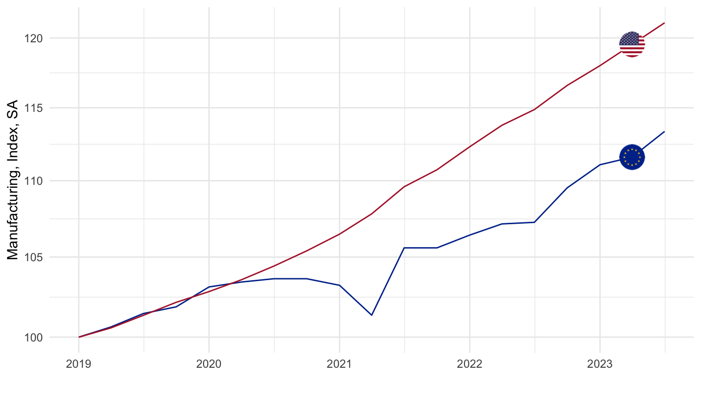
LCEAPR_IXOBSA
Code
EAR_MEI %>%
  filter(SUBJECT == "LCEAPR_IXOBSA",
         FREQUENCY == "Q",
         LOCATION %in% c("USA", "EA19")) %>%
  quarter_to_date %>%
  filter(date >= as.Date("2019-01-01")) %>%
  left_join(EAR_MEI_var$LOCATION, by = "LOCATION") %>%
  mutate(Location = ifelse(LOCATION == "EA19", "Europe", Location)) %>%
  left_join(colors, by = c("Location" = "country")) %>%
  mutate(color = ifelse(LOCATION == "USA", color2, color)) %>%
  group_by(Location) %>%
  arrange(date) %>%
  mutate(obsValue = 100*obsValue / obsValue[date == as.Date("2019-01-01")]) %>%
  ggplot(.) + geom_line(aes(x = date, y = obsValue, color = color)) +
  scale_color_identity() + theme_minimal() + add_2flags +
  scale_x_date(breaks = seq(1920, 2100, 1) %>% paste0("-01-01") %>% as.Date,
               labels = date_format("%Y")) +
  scale_y_log10(breaks = seq(10, 500, 5),
                     labels = scales::dollar_format(accuracy = 1, suffix = "", prefix = "")) +
  ylab("Private Sector, Index, SA") + xlab("")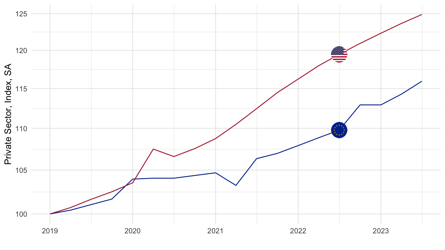
Eurozone, Japan, United States, United Kingdom
All
Code
EAR_MEI %>%
  filter(SUBJECT == "LCEAPR_IXOBSA",
         FREQUENCY == "Q",
         LOCATION %in% c("USA", "JPN", "EA19", "GBR", "HUN", "POL")) %>%
  quarter_to_date %>%
  left_join(EAR_MEI_var$LOCATION, by = "LOCATION") %>%
  mutate(Location = ifelse(LOCATION == "EA19", "Europe", Location)) %>%
  left_join(colors, by = c("Location" = "country")) %>%
  mutate(color = ifelse(LOCATION == "EA19", color2, color)) %>%
  ggplot(.) + geom_line(aes(x = date, y = obsValue, color = color)) +
  scale_color_identity() + theme_minimal() + add_6flags +
  scale_x_date(breaks = seq(1920, 2100, 2) %>% paste0("-01-01") %>% as.Date,
               labels = date_format("%Y")) +
  scale_y_log10(breaks = seq(10, 500, 10),
                     labels = scales::dollar_format(accuracy = 1, suffix = " k", prefix = "")) +
  ylab("Manufacturing, Index, SA") + xlab("")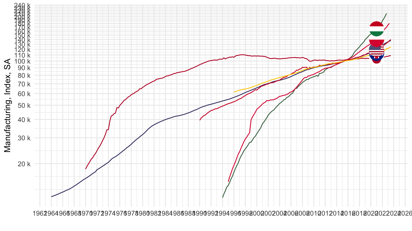
2015-
Code
EAR_MEI %>%
  filter(SUBJECT == "LCEAPR_IXOBSA",
         FREQUENCY == "Q",
         LOCATION %in% c("USA", "JPN", "EA19", "GBR", "HUN", "POL")) %>%
  quarter_to_date %>%
  filter(date >= as.Date("2015-01-01")) %>%
  left_join(EAR_MEI_var$LOCATION, by = "LOCATION") %>%
  mutate(Location = ifelse(LOCATION == "EA19", "Europe", Location)) %>%
  left_join(colors, by = c("Location" = "country")) %>%
  mutate(color = ifelse(LOCATION == "EA19", color2, color)) %>%
  group_by(Location) %>%
  mutate(obsValue = 100*obsValue / obsValue[date == as.Date("2015-01-01")]) %>%
  ggplot(.) + geom_line(aes(x = date, y = obsValue, color = color)) +
  scale_color_identity() + theme_minimal() + add_6flags +
  scale_x_date(breaks = seq(1920, 2100, 1) %>% paste0("-01-01") %>% as.Date,
               labels = date_format("%Y")) +
  scale_y_log10(breaks = seq(10, 500, 10),
                     labels = scales::dollar_format(accuracy = 1, suffix = "", prefix = "")) +
  ylab("Private Sector, Index, SA") + xlab("")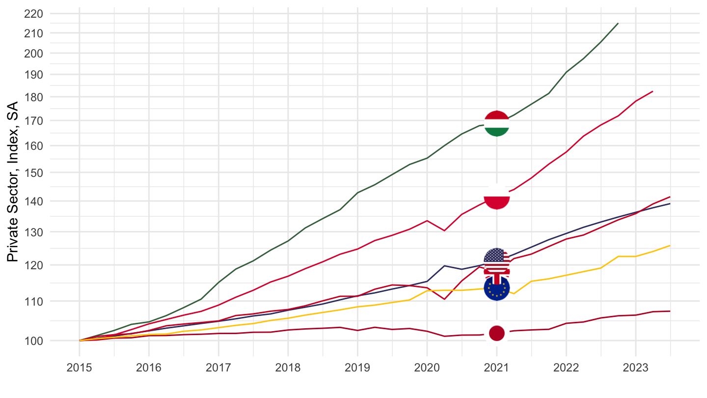
Eurozone, United States, United Kingdom
All
Code
EAR_MEI %>%
  filter(SUBJECT == "LCEAPR_IXOBSA",
         FREQUENCY == "Q",
         LOCATION %in% c("USA", "EA19", "GBR")) %>%
  quarter_to_date %>%
  left_join(EAR_MEI_var$LOCATION, by = "LOCATION") %>%
  left_join(PRICES_CPI_CPALTT01_IXOB, by = c("date", "Location", "LOCATION")) %>%
  mutate(Location = ifelse(LOCATION == "EA19", "Europe", Location)) %>%
  left_join(colors, by = c("Location" = "country")) %>%
  mutate(color = ifelse(LOCATION == "EA19", color2, color)) %>%
  ggplot(.) + geom_line(aes(x = date, y = obsValue, color = color)) +
  scale_color_identity() + theme_minimal() + add_3flags +
  scale_x_date(breaks = seq(1920, 2100, 5) %>% paste0("-01-01") %>% as.Date,
               labels = date_format("%Y")) +
  scale_y_log10(breaks = seq(10, 500, 10),
                     labels = scales::dollar_format(accuracy = 1, suffix = " k", prefix = "")) +
  ylab("Manufacturing, Index, SA") + xlab("")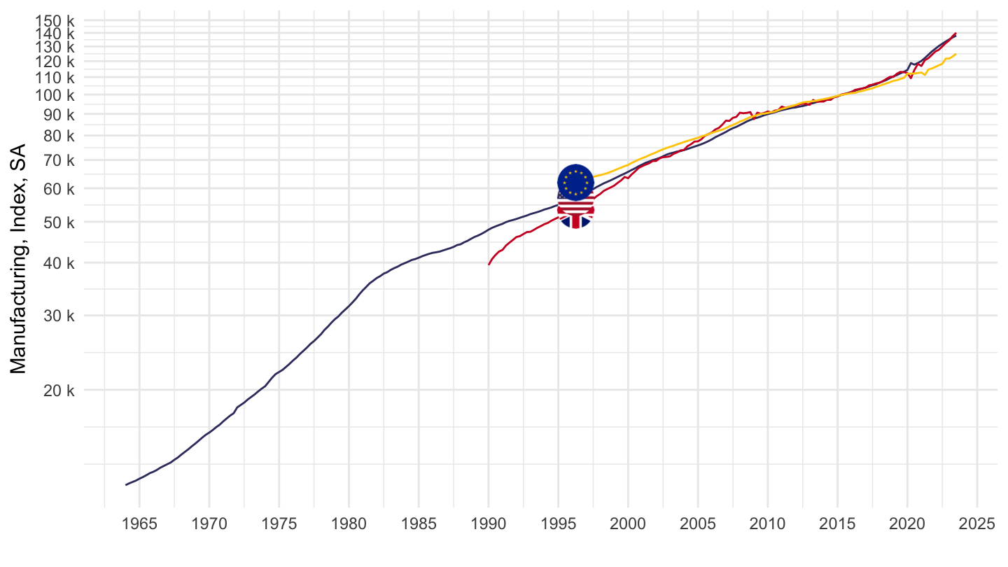
1996-
Nominal
Code
EAR_MEI %>%
  filter(SUBJECT == "LCEAPR_IXOBSA",
         FREQUENCY == "Q",
         LOCATION %in% c("USA", "EA19", "GBR")) %>%
  quarter_to_date %>%
  filter(date >= as.Date("1996-01-01")) %>%
  left_join(EAR_MEI_var$LOCATION, by = "LOCATION") %>%
  left_join(PRICES_CPI_CPALTT01_IXOB, by = c("date", "Location", "LOCATION")) %>%
  mutate(Location = ifelse(LOCATION == "EA19", "Europe", Location)) %>%
  left_join(colors, by = c("Location" = "country")) %>%
  mutate(color = ifelse(LOCATION == "EA19", color2, color)) %>%
  group_by(Location) %>%
  mutate(obsValue = 100*obsValue / obsValue[date == as.Date("1996-01-01")]) %>%
  ggplot(.) + geom_line(aes(x = date, y = obsValue, color = color)) +
  scale_color_identity() + theme_minimal() + add_3flags +
  scale_x_date(breaks = seq(1920, 2100, 2) %>% paste0("-01-01") %>% as.Date,
               labels = date_format("%Y")) +
  scale_y_log10(breaks = seq(10, 500, 5),
                     labels = scales::dollar_format(accuracy = 1, suffix = "", prefix = "")) +
  ylab("Private Sector, Index, SA") + xlab("")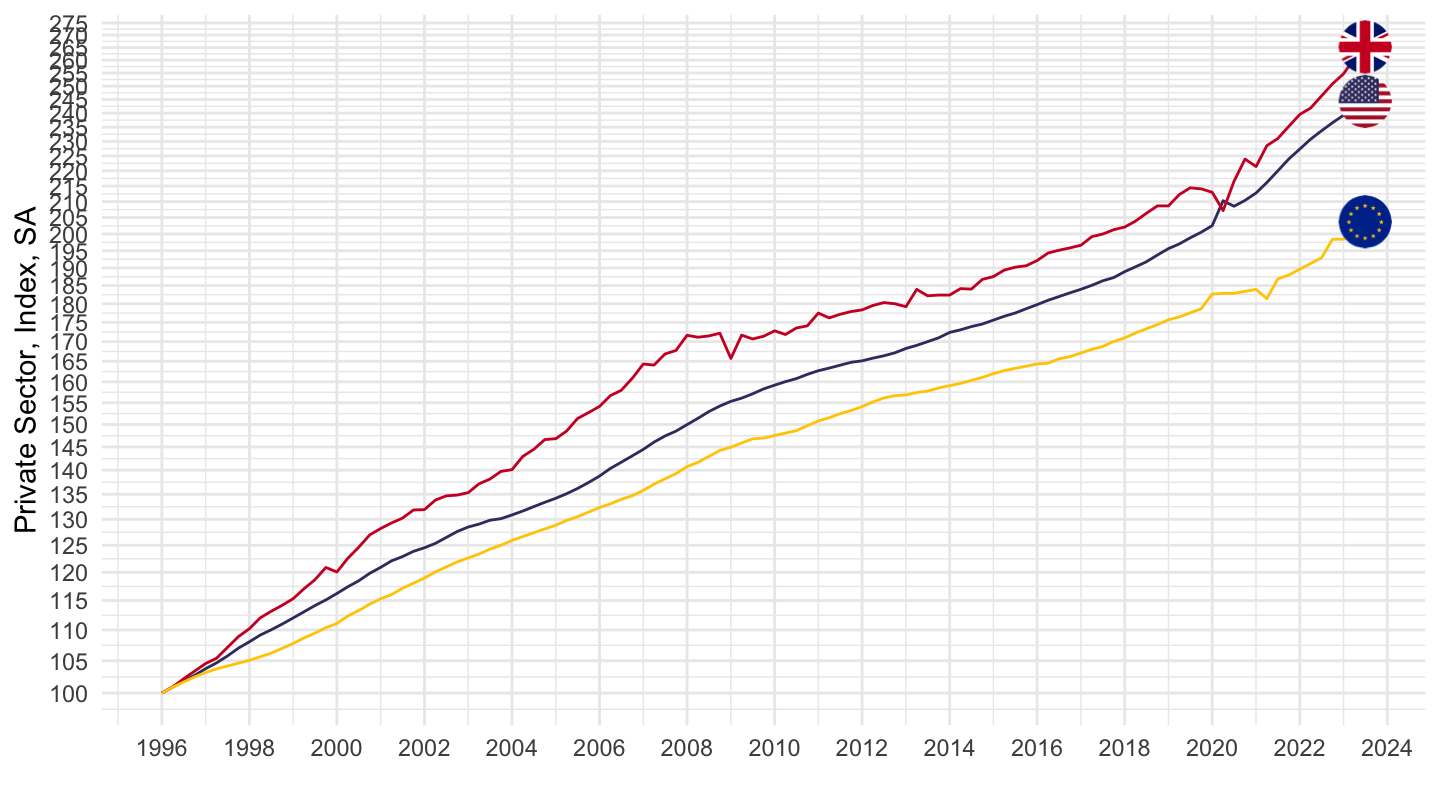
Real
Code
EAR_MEI %>%
  filter(SUBJECT == "LCEAPR_IXOBSA",
         FREQUENCY == "Q",
         LOCATION %in% c("USA", "EA19")) %>%
  quarter_to_date %>%
  filter(date >= as.Date("1996-01-01")) %>%
  left_join(EAR_MEI_var$LOCATION, by = "LOCATION") %>%
  left_join(PRICES_CPI_CPALTT01_IXOB, by = c("date", "Location", "LOCATION")) %>%
  mutate(Location = ifelse(LOCATION == "EA19", "Europe", Location)) %>%
  mutate(obsValue = obsValue/CPALTT01_IXOB) %>%
  left_join(colors, by = c("Location" = "country")) %>%
  mutate(color = ifelse(LOCATION == "EA19", color2, color)) %>%
  group_by(Location) %>%
  mutate(obsValue = 100*obsValue / obsValue[date == as.Date("1996-01-01")]) %>%
  ggplot(.) + geom_line(aes(x = date, y = obsValue, color = color)) +
  scale_color_identity() + theme_minimal() + add_2flags +
  scale_x_date(breaks = seq(1920, 2100, 2) %>% paste0("-01-01") %>% as.Date,
               labels = date_format("%Y")) + add_6flags +
  scale_y_log10(breaks = seq(10, 500, 5),
                     labels = scales::dollar_format(accuracy = 1, suffix = "", prefix = "")) +
  ylab("Private Sector, Index, SA") + xlab("")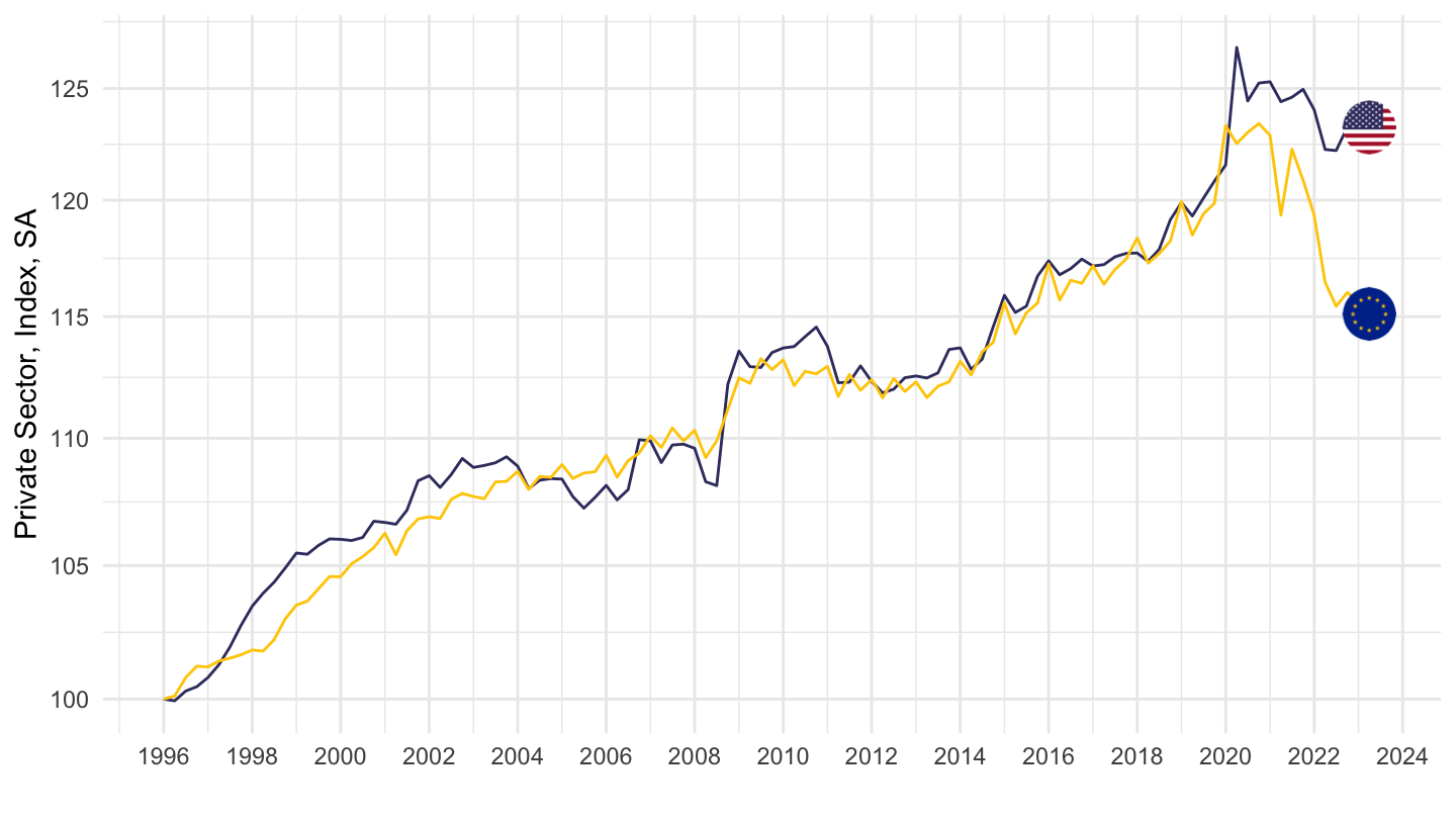
2015-
Nominal
Code
EAR_MEI %>%
  filter(SUBJECT == "LCEAPR_IXOBSA",
         FREQUENCY == "Q",
         LOCATION %in% c("USA", "EA19", "GBR")) %>%
  quarter_to_date %>%
  filter(date >= as.Date("2015-01-01")) %>%
  left_join(EAR_MEI_var$LOCATION, by = "LOCATION") %>%
  mutate(Location = ifelse(LOCATION == "EA19", "Europe", Location)) %>%
  left_join(colors, by = c("Location" = "country")) %>%
  mutate(color = ifelse(LOCATION == "EA19", color2, color)) %>%
  group_by(Location) %>%
  mutate(obsValue = 100*obsValue / obsValue[date == as.Date("2015-01-01")]) %>%
  ggplot(.) + geom_line(aes(x = date, y = obsValue, color = color)) +
  scale_color_identity() + theme_minimal() + add_3flags +
  scale_x_date(breaks = seq(1920, 2100, 1) %>% paste0("-01-01") %>% as.Date,
               labels = date_format("%Y")) + add_6flags +
  scale_y_log10(breaks = seq(10, 500, 5),
                     labels = scales::dollar_format(accuracy = 1, suffix = "", prefix = "")) +
  ylab("Private Sector, Index, SA") + xlab("")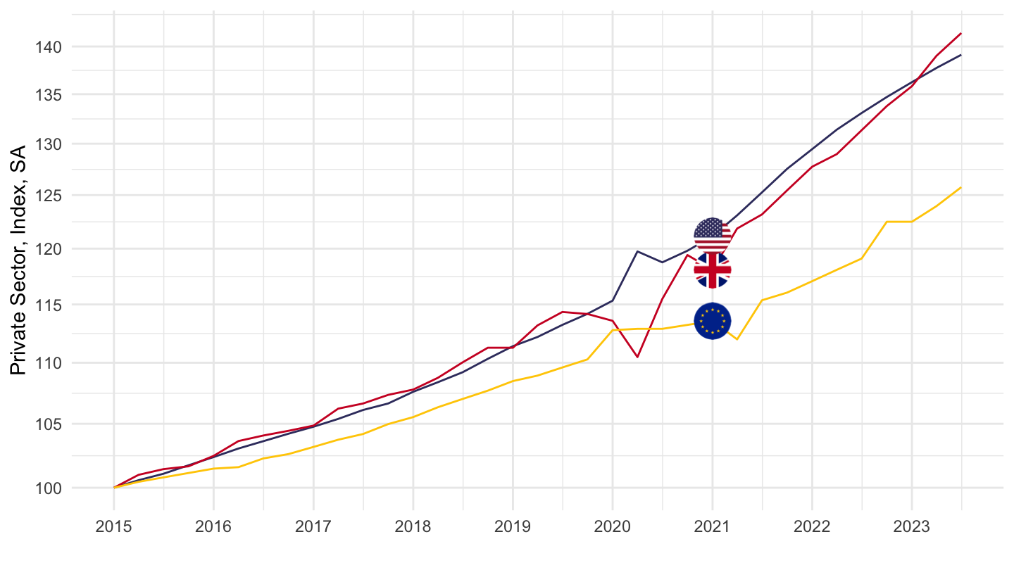
Real
All
Code
EAR_MEI %>%
  filter(SUBJECT == "LCEAPR_IXOBSA",
         FREQUENCY == "Q",
         LOCATION %in% c("USA", "EA19", "GBR")) %>%
  quarter_to_date %>%
  filter(date >= as.Date("2015-01-01")) %>%
  left_join(EAR_MEI_var$LOCATION, by = "LOCATION") %>%
  left_join(PRICES_CPI_CPALTT01_IXOB, by = c("date", "Location", "LOCATION")) %>%
  mutate(Location = ifelse(LOCATION == "EA19", "Europe", Location)) %>%
  mutate(obsValue = obsValue/CPALTT01_IXOB) %>%
  left_join(colors, by = c("Location" = "country")) %>%
  mutate(color = ifelse(LOCATION == "EA19", color2, color)) %>%
  group_by(Location) %>%
  mutate(obsValue = 100*obsValue / obsValue[date == as.Date("2015-01-01")]) %>%
  ggplot(.) + geom_line(aes(x = date, y = obsValue, color = color)) +
  scale_color_identity() + theme_minimal() + add_3flags +
  scale_x_date(breaks = seq(1920, 2100, 1) %>% paste0("-01-01") %>% as.Date,
               labels = date_format("%Y")) + add_6flags +
  scale_y_log10(breaks = seq(10, 500, 1),
                     labels = scales::dollar_format(accuracy = 1, suffix = "", prefix = "")) +
  ylab("Private Sector, Index, SA, Real") + xlab("")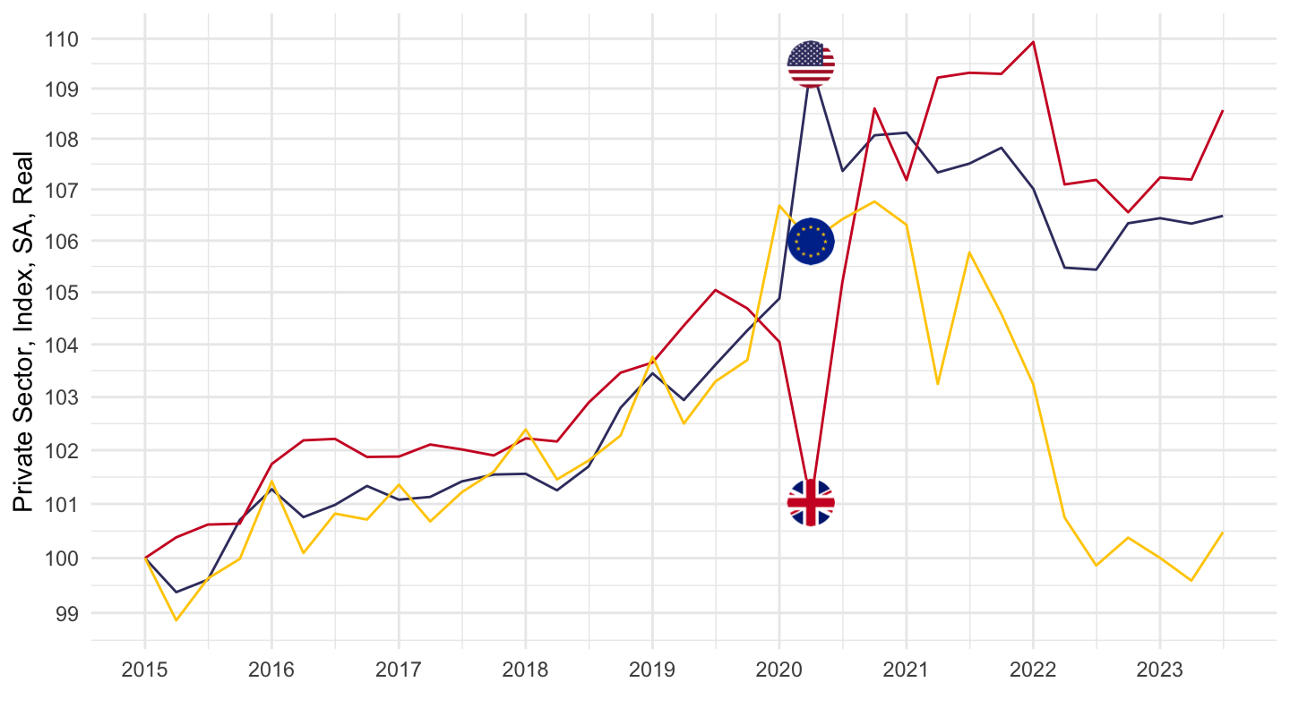
2019-
Nominal
Code
EAR_MEI %>%
  filter(SUBJECT == "LCEAPR_IXOBSA",
         FREQUENCY == "Q",
         LOCATION %in% c("USA", "EA19", "GBR")) %>%
  quarter_to_date %>%
  filter(date >= as.Date("2019-01-01")) %>%
  left_join(EAR_MEI_var$LOCATION, by = "LOCATION") %>%
  mutate(Location = ifelse(LOCATION == "EA19", "Europe", Location)) %>%
  left_join(colors, by = c("Location" = "country")) %>%
  mutate(color = ifelse(LOCATION == "EA19", color2, color)) %>%
  group_by(Location) %>%
  arrange(date) %>%
  mutate(obsValue = 100*obsValue / obsValue[date == as.Date("2019-01-01")]) %>%
  ggplot(.) + geom_line(aes(x = date, y = obsValue, color = color)) +
  scale_color_identity() + theme_minimal() + add_3flags +
  scale_x_date(breaks = seq(1920, 2100, 1) %>% paste0("-01-01") %>% as.Date,
               labels = date_format("%Y")) +
  scale_y_log10(breaks = seq(10, 500, 5),
                     labels = scales::dollar_format(accuracy = 1, suffix = "", prefix = "")) +
  ylab("Private Sector, Index, SA") + xlab("")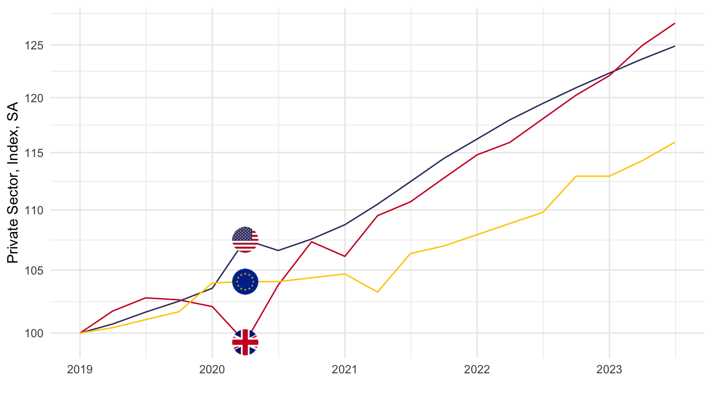
Real
All
Code
EAR_MEI %>%
  filter(SUBJECT == "LCEAPR_IXOBSA",
         FREQUENCY == "Q",
         LOCATION %in% c("USA", "EA19", "GBR")) %>%
  quarter_to_date %>%
  filter(date >= as.Date("2019-01-01")) %>%
  left_join(EAR_MEI_var$LOCATION, by = "LOCATION") %>%
  left_join(PRICES_CPI_CPALTT01_IXOB, by = c("date", "Location", "LOCATION")) %>%
  mutate(Location = ifelse(LOCATION == "EA19", "Europe", Location)) %>%
  mutate(obsValue = obsValue/CPALTT01_IXOB) %>%
  left_join(colors, by = c("Location" = "country")) %>%
  mutate(color = ifelse(LOCATION == "EA19", color2, color)) %>%
  group_by(Location) %>%
  mutate(obsValue = 100*obsValue / obsValue[date == as.Date("2019-01-01")]) %>%
  ggplot(.) + geom_line(aes(x = date, y = obsValue, color = color)) +
  scale_color_identity() + theme_minimal() + add_3flags +
  scale_x_date(breaks = seq(1920, 2100, 1) %>% paste0("-01-01") %>% as.Date,
               labels = date_format("%Y")) +
  scale_y_log10(breaks = seq(10, 500, 1),
                     labels = scales::dollar_format(accuracy = 1, suffix = "", prefix = "")) +
  ylab("Private Sector, Index, SA, Real") + xlab("")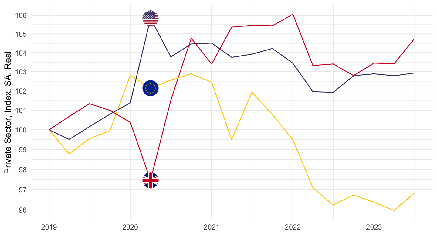
Eurozone, United States, United Kingdom, France, Germany, Italy, Belgium
2015-
Nominal
Code
EAR_MEI %>%
  filter(SUBJECT == "LCEAPR_IXOBSA",
         FREQUENCY == "Q",
         LOCATION %in% c("USA", "DEU", "BEL")) %>%
  quarter_to_date %>%
  filter(date >= as.Date("2015-01-01")) %>%
  left_join(EAR_MEI_var$LOCATION, by = "LOCATION") %>%
  mutate(Location = ifelse(LOCATION == "EA19", "Europe", Location)) %>%
  left_join(colors, by = c("Location" = "country")) %>%
  mutate(color = ifelse(LOCATION == "EA19", color2, color)) %>%
  group_by(Location) %>%
  mutate(obsValue = 100*obsValue / obsValue[date == as.Date("2015-01-01")]) %>%
  ggplot(.) + geom_line(aes(x = date, y = obsValue, color = color)) +
  scale_color_identity() + theme_minimal() + add_3flags +
  scale_x_date(breaks = seq(1920, 2100, 1) %>% paste0("-01-01") %>% as.Date,
               labels = date_format("%Y")) + add_6flags +
  scale_y_log10(breaks = seq(10, 500, 5),
                     labels = scales::dollar_format(accuracy = 1, suffix = "", prefix = "")) +
  ylab("Private Sector, Index, SA") + xlab("")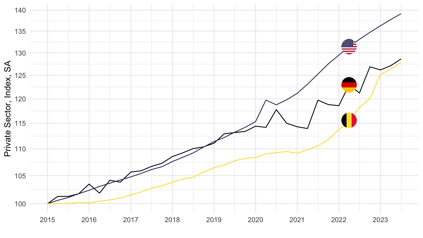
Real
Code
EAR_MEI %>%
  filter(SUBJECT == "LCEAPR_IXOBSA",
         FREQUENCY == "Q",
         LOCATION %in% c("USA", "DEU", "BEL")) %>%
  quarter_to_date %>%
  filter(date >= as.Date("2015-01-01")) %>%
  left_join(EAR_MEI_var$LOCATION, by = "LOCATION") %>%
  left_join(PRICES_CPI_CPALTT01_IXOB, by = c("date", "Location", "LOCATION")) %>%
  mutate(Location = ifelse(LOCATION == "EA19", "Europe", Location)) %>%
  mutate(obsValue = obsValue/CPALTT01_IXOB) %>%
  left_join(colors, by = c("Location" = "country")) %>%
  mutate(color = ifelse(LOCATION == "EA19", color2, color)) %>%
  group_by(Location) %>%
  mutate(obsValue = 100*obsValue / obsValue[date == as.Date("2015-01-01")]) %>%
  ggplot(.) + geom_line(aes(x = date, y = obsValue, color = color)) +
  scale_color_identity() + theme_minimal() + add_3flags +
  scale_x_date(breaks = seq(1920, 2100, 1) %>% paste0("-01-01") %>% as.Date,
               labels = date_format("%Y")) + add_6flags +
  scale_y_log10(breaks = seq(10, 500, 1),
                     labels = scales::dollar_format(accuracy = 1, suffix = "", prefix = "")) +
  ylab("Private Sector, Index, SA, Real") + xlab("")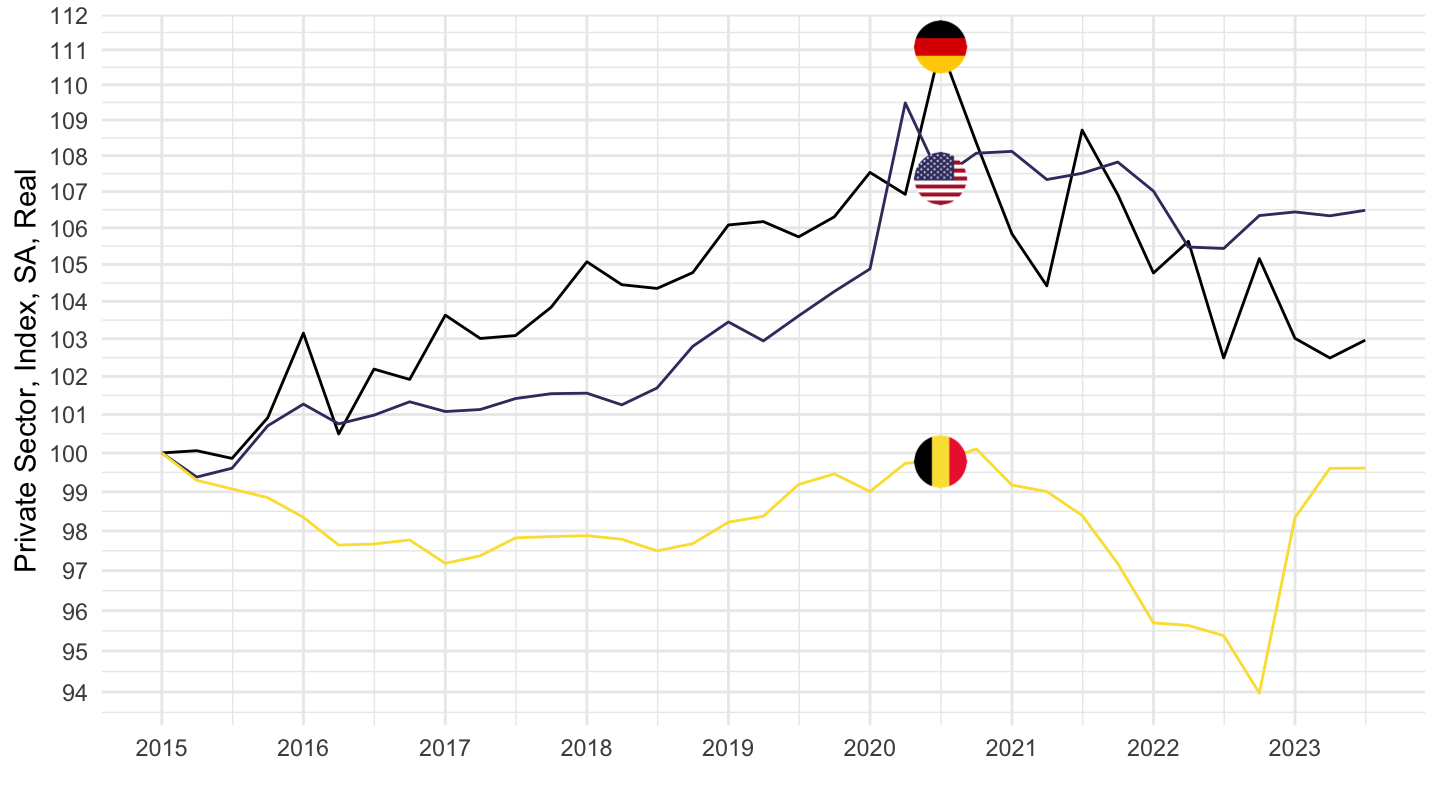
Poland, Hungary
2015-
Nominal
Code
EAR_MEI %>%
  filter(SUBJECT == "LCEAPR_IXOBSA",
         FREQUENCY == "Q",
         LOCATION %in% c("POL", "HUN")) %>%
  quarter_to_date %>%
  filter(date >= as.Date("2015-01-01")) %>%
  left_join(EAR_MEI_var$LOCATION, by = "LOCATION") %>%
  mutate(Location = ifelse(LOCATION == "EA19", "Europe", Location)) %>%
  left_join(colors, by = c("Location" = "country")) %>%
  mutate(color = ifelse(LOCATION == "FRA", color2, color)) %>%
  group_by(Location) %>%
  mutate(obsValue = 100*obsValue / obsValue[date == as.Date("2015-01-01")]) %>%
  ggplot(.) + geom_line(aes(x = date, y = obsValue, color = color)) +
  scale_color_identity() + theme_minimal() +
  scale_x_date(breaks = seq(1920, 2100, 1) %>% paste0("-01-01") %>% as.Date,
               labels = date_format("%Y")) + add_2flags +
  scale_y_log10(breaks = seq(10, 500, 5),
                     labels = scales::dollar_format(accuracy = 1, suffix = "", prefix = "")) +
  ylab("Private Sector, Index, SA") + xlab("")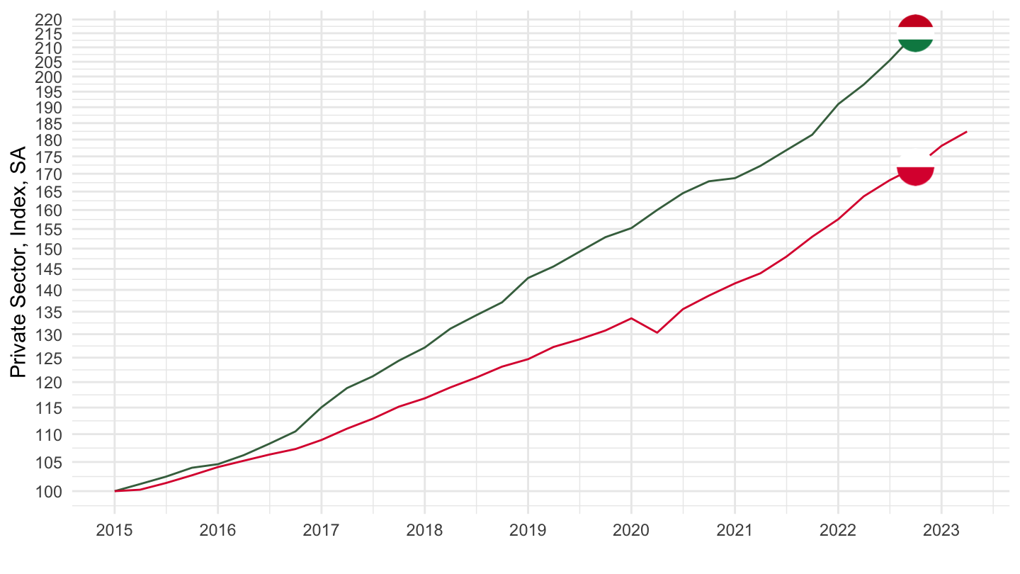
Real
Code
EAR_MEI %>%
  filter(SUBJECT == "LCEAPR_IXOBSA",
         FREQUENCY == "Q",
         LOCATION %in% c("POL", "HUN")) %>%
  quarter_to_date %>%
  filter(date >= as.Date("2015-01-01")) %>%
  left_join(EAR_MEI_var$LOCATION, by = "LOCATION") %>%
  left_join(PRICES_CPI_CPALTT01_IXOB, by = c("date", "Location", "LOCATION")) %>%
  mutate(Location = ifelse(LOCATION == "EA19", "Europe", Location)) %>%
  mutate(obsValue = obsValue/CPALTT01_IXOB) %>%
  left_join(colors, by = c("Location" = "country")) %>%
  mutate(color = ifelse(LOCATION == "FRA", color2, color)) %>%
  group_by(Location) %>%
  mutate(obsValue = 100*obsValue / obsValue[date == as.Date("2015-01-01")]) %>%
  ggplot(.) + geom_line(aes(x = date, y = obsValue, color = color)) +
  scale_color_identity() + theme_minimal() + add_2flags +
  scale_x_date(breaks = seq(1920, 2100, 1) %>% paste0("-01-01") %>% as.Date,
               labels = date_format("%Y")) +
  scale_y_log10(breaks = seq(10, 500, 5),
                     labels = scales::dollar_format(accuracy = 1, suffix = "", prefix = "")) +
  ylab("Private Sector, Index, SA, Real") + xlab("")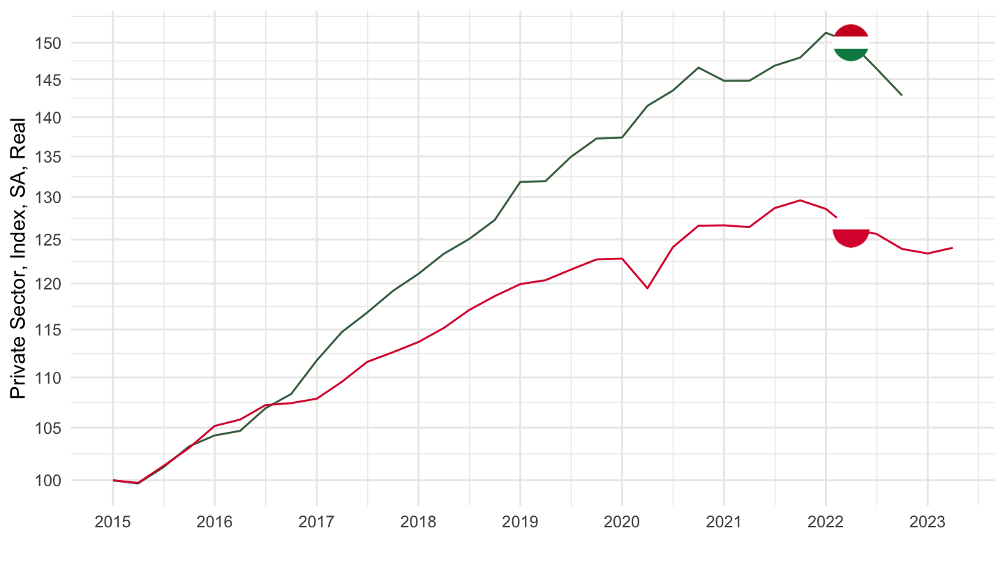
Sweden, Netherlands, Luxembourg, Hungary, Poland, Finland
2015-
Nominal
Code
EAR_MEI %>%
  filter(SUBJECT == "LCEAPR_IXOBSA",
         FREQUENCY == "Q",
         LOCATION %in% c("SWE", "NLD", "LUX", "FIN", "DNK", "IRL")) %>%
  quarter_to_date %>%
  filter(date >= as.Date("2015-01-01")) %>%
  left_join(EAR_MEI_var$LOCATION, by = "LOCATION") %>%
  mutate(Location = ifelse(LOCATION == "EA19", "Europe", Location)) %>%
  left_join(colors, by = c("Location" = "country")) %>%
  mutate(color = ifelse(LOCATION == "FRA", color2, color)) %>%
  group_by(Location) %>%
  mutate(obsValue = 100*obsValue / obsValue[date == as.Date("2015-01-01")]) %>%
  ggplot(.) + geom_line(aes(x = date, y = obsValue, color = color)) +
  scale_color_identity() + theme_minimal() +
  scale_x_date(breaks = seq(1920, 2100, 1) %>% paste0("-01-01") %>% as.Date,
               labels = date_format("%Y")) + add_4flags +
  scale_y_log10(breaks = seq(10, 500, 5),
                     labels = scales::dollar_format(accuracy = 1, suffix = "", prefix = "")) +
  ylab("Private Sector, Index, SA") + xlab("")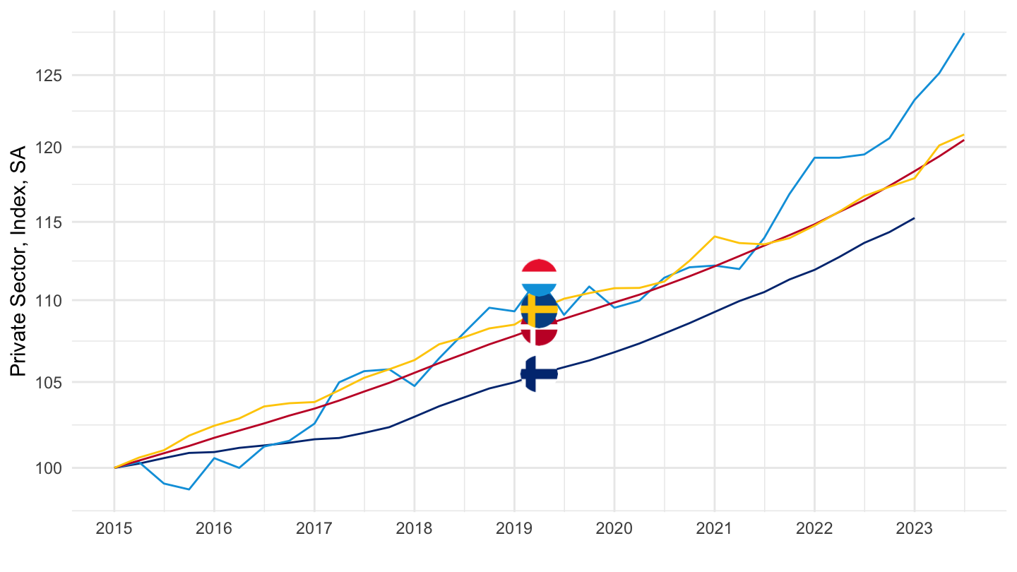
Real
Code
EAR_MEI %>%
  filter(SUBJECT == "LCEAPR_IXOBSA",
         FREQUENCY == "Q",
         LOCATION %in% c("SWE", "NLD", "LUX", "FIN", "DNK", "IRL")) %>%
  quarter_to_date %>%
  filter(date >= as.Date("2015-01-01")) %>%
  left_join(EAR_MEI_var$LOCATION, by = "LOCATION") %>%
  left_join(PRICES_CPI_CPALTT01_IXOB, by = c("date", "Location", "LOCATION")) %>%
  mutate(Location = ifelse(LOCATION == "EA19", "Europe", Location)) %>%
  mutate(obsValue = obsValue/CPALTT01_IXOB) %>%
  left_join(colors, by = c("Location" = "country")) %>%
  mutate(color = ifelse(LOCATION == "FRA", color2, color)) %>%
  group_by(Location) %>%
  mutate(obsValue = 100*obsValue / obsValue[date == as.Date("2015-01-01")]) %>%
  ggplot(.) + geom_line(aes(x = date, y = obsValue, color = color)) +
  scale_color_identity() + theme_minimal() + add_4flags +
  scale_x_date(breaks = seq(1920, 2100, 1) %>% paste0("-01-01") %>% as.Date,
               labels = date_format("%Y")) +
  scale_y_log10(breaks = seq(10, 500, 1),
                     labels = scales::dollar_format(accuracy = 1, suffix = "", prefix = "")) +
  ylab("Private Sector, Index, SA, Real") + xlab("")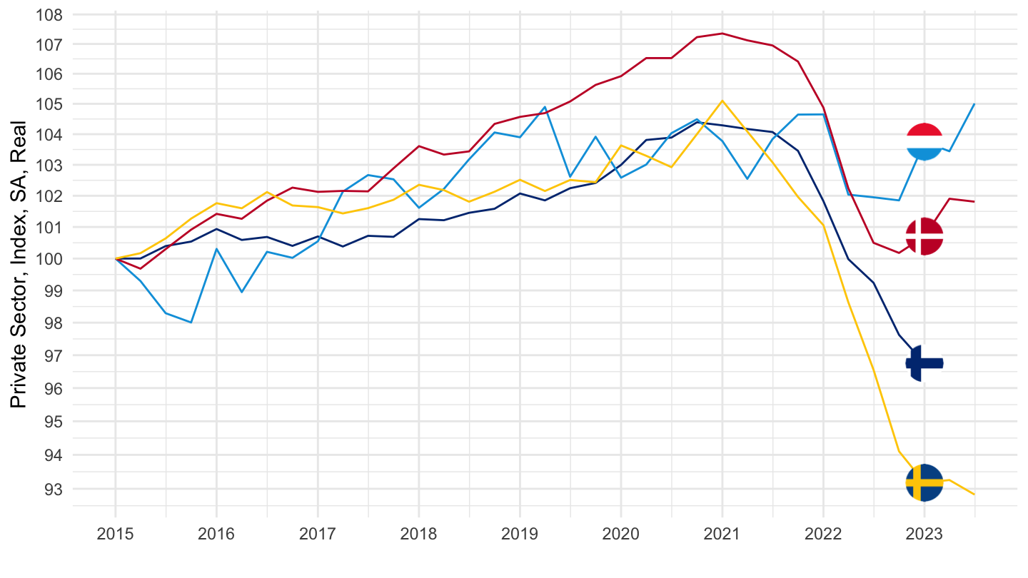
Eurozone, United States, United Kingdom, France, Germany, Italy, Belgium
2015-
Nominal
Code
EAR_MEI %>%
  filter(SUBJECT == "LCEAPR_IXOBSA",
         FREQUENCY == "Q",
         LOCATION %in% c("FRA", "DEU", "ITA", "BEL", "ESP", "PRT", "AUT")) %>%
  quarter_to_date %>%
  filter(date >= as.Date("2015-01-01")) %>%
  left_join(EAR_MEI_var$LOCATION, by = "LOCATION") %>%
  mutate(Location = ifelse(LOCATION == "EA19", "Europe", Location)) %>%
  left_join(colors, by = c("Location" = "country")) %>%
  mutate(color = ifelse(LOCATION == "FRA", color2, color)) %>%
  group_by(Location) %>%
  mutate(obsValue = 100*obsValue / obsValue[date == as.Date("2015-01-01")]) %>%
  ggplot(.) + geom_line(aes(x = date, y = obsValue, color = color)) +
  scale_color_identity() + theme_minimal() +
  scale_x_date(breaks = seq(1920, 2100, 1) %>% paste0("-01-01") %>% as.Date,
               labels = date_format("%Y")) + add_6flags +
  scale_y_log10(breaks = seq(10, 500, 5),
                     labels = scales::dollar_format(accuracy = 1, suffix = "", prefix = "")) +
  ylab("Private Sector, Index, SA") + xlab("")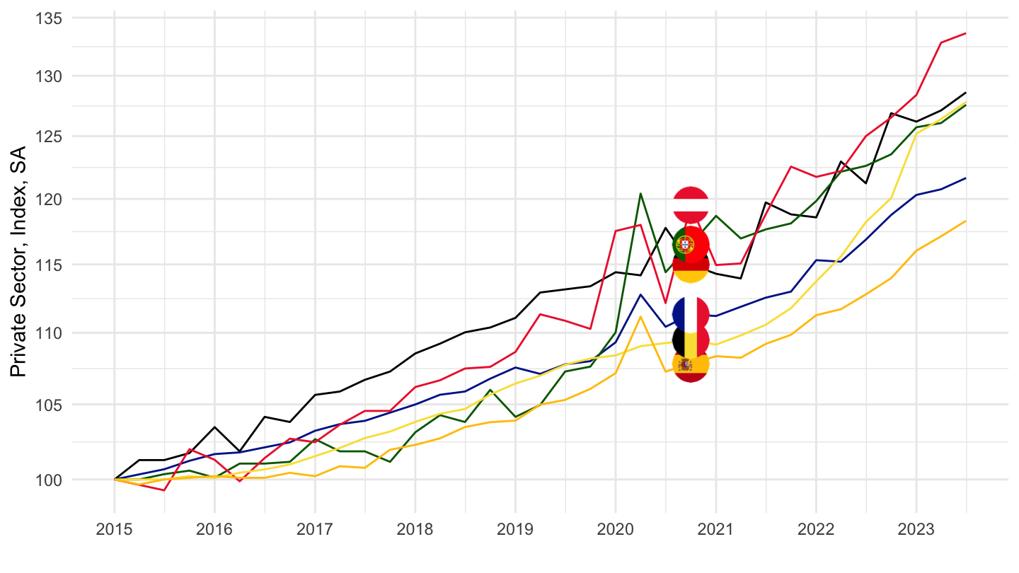
Real
Code
EAR_MEI %>%
  filter(SUBJECT == "LCEAPR_IXOBSA",
         FREQUENCY == "Q",
         LOCATION %in% c("FRA", "DEU", "ITA", "BEL", "ESP", "PRT", "AUT")) %>%
  quarter_to_date %>%
  filter(date >= as.Date("2015-01-01")) %>%
  left_join(EAR_MEI_var$LOCATION, by = "LOCATION") %>%
  left_join(PRICES_CPI_CPALTT01_IXOB, by = c("date", "Location", "LOCATION")) %>%
  mutate(Location = ifelse(LOCATION == "EA19", "Europe", Location)) %>%
  mutate(obsValue = obsValue/CPALTT01_IXOB) %>%
  left_join(colors, by = c("Location" = "country")) %>%
  mutate(color = ifelse(LOCATION == "FRA", color2, color)) %>%
  group_by(Location) %>%
  mutate(obsValue = 100*obsValue / obsValue[date == as.Date("2015-01-01")]) %>%
  ggplot(.) + geom_line(aes(x = date, y = obsValue, color = color)) +
  scale_color_identity() + theme_minimal() + add_6flags +
  scale_x_date(breaks = seq(1920, 2100, 1) %>% paste0("-01-01") %>% as.Date,
               labels = date_format("%Y")) +
  scale_y_log10(breaks = seq(10, 500, 1),
                     labels = scales::dollar_format(accuracy = 1, suffix = "", prefix = "")) +
  ylab("Private Sector, Index, SA, Real") + xlab("")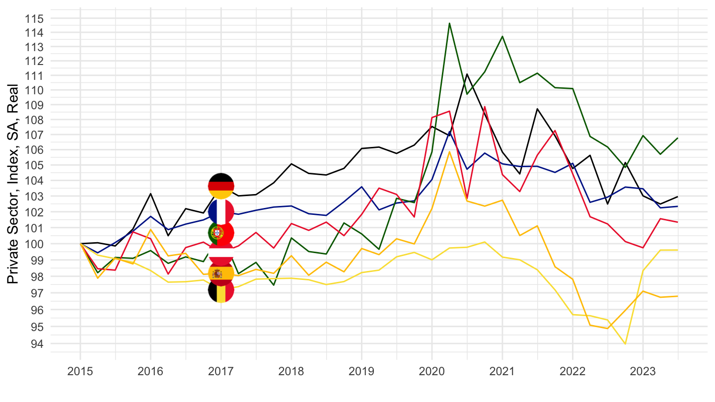
2020-
Nominal
Code
EAR_MEI %>%
  filter(SUBJECT == "LCEAPR_IXOBSA",
         FREQUENCY == "Q",
         LOCATION %in% c("FRA", "DEU", "ITA", "BEL", "ESP", "PRT", "AUT")) %>%
  quarter_to_date %>%
  filter(date >= as.Date("2019-10-01")) %>%
  left_join(EAR_MEI_var$LOCATION, by = "LOCATION") %>%
  mutate(Location = ifelse(LOCATION == "EA19", "Europe", Location)) %>%
  left_join(colors, by = c("Location" = "country")) %>%
  mutate(color = ifelse(LOCATION == "FRA", color2, color)) %>%
  group_by(Location) %>%
  mutate(obsValue = 100*obsValue / obsValue[date == as.Date("2019-10-01")]) %>%
  ggplot(.) + geom_line(aes(x = date, y = obsValue, color = color)) +
  scale_color_identity() + theme_minimal() + add_6flags +
  theme(axis.text.x = element_text(angle = 45, vjust = 1, hjust = 1)) +
  scale_x_date(breaks = seq(as.Date("2015-01-01"), Sys.Date(), "3 months"),
               labels = date_format("%b %Y")) +
  scale_y_log10(breaks = seq(10, 500, 5),
                     labels = scales::dollar_format(accuracy = 1, suffix = "", prefix = "")) +
  ylab("Private Sector, Index, SA") + xlab("")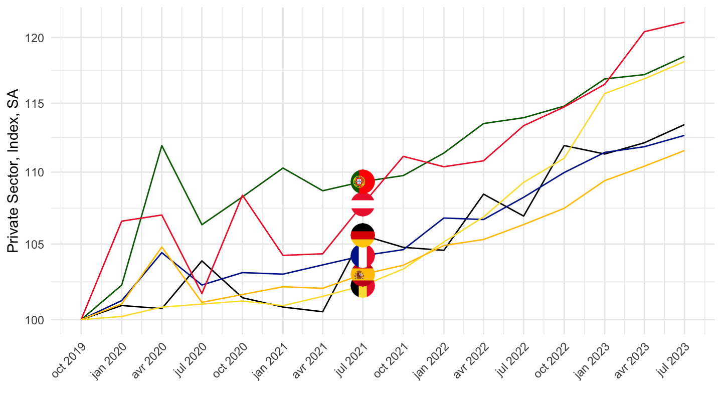
Real
Code
df <- EAR_MEI %>%
  filter(SUBJECT == "LCEAPR_IXOBSA",
         FREQUENCY == "Q",
         LOCATION %in% c("FRA", "DEU", "ITA", "BEL", "ESP", "PRT", "AUT")) %>%
  quarter_to_date %>%
  filter(date >= as.Date("2019-10-01")) %>%
  left_join(EAR_MEI_var$LOCATION, by = "LOCATION") %>%
  left_join(PRICES_CPI_CPALTT01_IXOB, by = c("date", "Location", "LOCATION")) %>%
  mutate(Location = ifelse(LOCATION == "EA19", "Europe", Location)) %>%
  mutate(obsValue = obsValue/CPALTT01_IXOB) %>%
  left_join(colors, by = c("Location" = "country")) %>%
  mutate(color = ifelse(LOCATION == "FRA", color2, color)) %>%
  group_by(Location) %>%
  mutate(obsValue = 100*obsValue / obsValue[date == as.Date("2019-10-01")]) %>%
  mutate(date = zoo::as.yearqtr(paste0(year(date), " Q", quarter(date))))

  ggplot(data = df) + geom_line(aes(x = date, y = obsValue, color = color)) +
  scale_color_identity() + theme_minimal() + add_6flags +
  theme(axis.text.x = element_text(angle = 45, vjust = 1, hjust = 1)) +
  scale_x_yearqtr(labels = date_format("%Y Q%q"),
                  breaks = seq(from = min(df$date), to = max(df$date), by = 0.25)) +
  scale_y_log10(breaks = seq(10, 500, 1),
                     labels = scales::dollar_format(accuracy = 1, suffix = "", prefix = "")) +
  ylab("Private Sector, Index, SA, Real") + xlab("")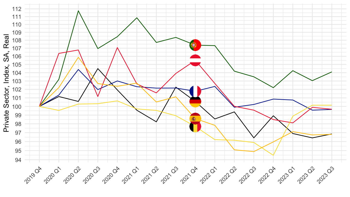
2022-
Real
Code
df <- EAR_MEI %>%
  filter(SUBJECT == "LCEAPR_IXOBSA",
         FREQUENCY == "Q",
         LOCATION %in% c("FRA", "DEU", "ITA", "BEL", "ESP", "PRT", "AUT")) %>%
  quarter_to_date %>%
  filter(date >= as.Date("2021-10-01")) %>%
  left_join(EAR_MEI_var$LOCATION, by = "LOCATION") %>%
  left_join(PRICES_CPI_CPALTT01_IXOB, by = c("date", "Location", "LOCATION")) %>%
  mutate(Location = ifelse(LOCATION == "EA19", "Europe", Location)) %>%
  mutate(obsValue = obsValue/CPALTT01_IXOB) %>%
  left_join(colors, by = c("Location" = "country")) %>%
  mutate(color = ifelse(LOCATION == "FRA", color2, color)) %>%
  group_by(Location) %>%
  mutate(obsValue = 100*obsValue / obsValue[date == as.Date("2021-10-01")]) %>%
  mutate(date = zoo::as.yearqtr(paste0(year(date), " Q", quarter(date))))

  ggplot(data = df) + geom_line(aes(x = date, y = obsValue, color = color)) +
  scale_color_identity() + theme_minimal() + add_6flags +
  theme(axis.text.x = element_text(angle = 45, vjust = 1, hjust = 1)) +
  scale_x_yearqtr(labels = date_format("%Y Q%q"),
                  breaks = seq(from = min(df$date), to = max(df$date), by = 0.25)) +
  scale_y_log10(breaks = seq(10, 500, 1),
                     labels = scales::dollar_format(accuracy = 1, suffix = "", prefix = "")) +
  ylab("Private Sector, Index, SA, Real") + xlab("")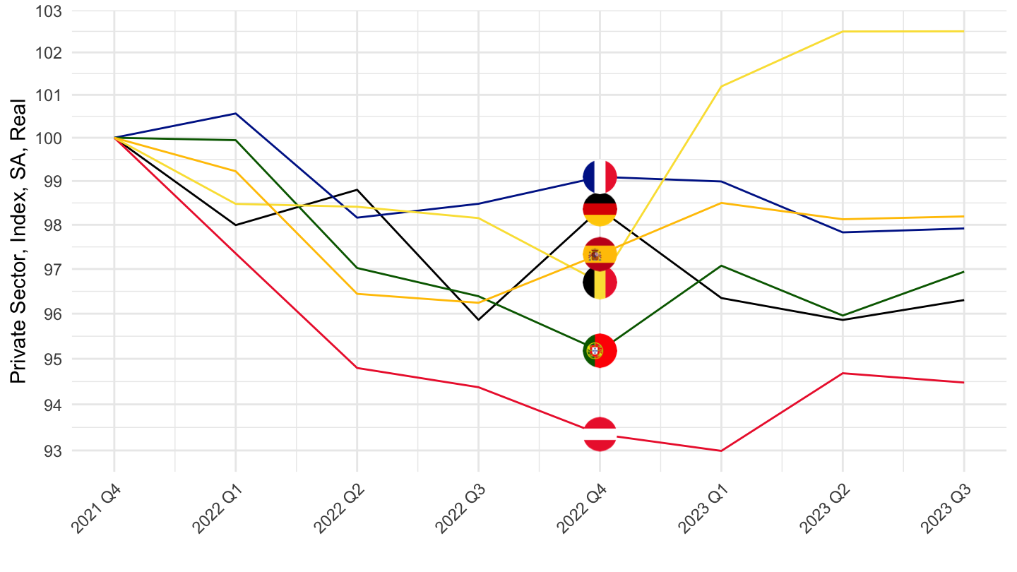
Eurozone, United States, United Kingdom, France
2015-
Nominal
Code
EAR_MEI %>%
  filter(SUBJECT == "LCEAPR_IXOBSA",
         FREQUENCY == "Q",
         LOCATION %in% c("USA", "EA19", "GBR", "FRA")) %>%
  quarter_to_date %>%
  filter(date >= as.Date("2015-01-01")) %>%
  left_join(EAR_MEI_var$LOCATION, by = "LOCATION") %>%
  mutate(Location = ifelse(LOCATION == "EA19", "Europe", Location)) %>%
  left_join(colors, by = c("Location" = "country")) %>%
  mutate(color = ifelse(LOCATION == "EA19", color2, color)) %>%
  group_by(Location) %>%
  mutate(obsValue = 100*obsValue / obsValue[date == as.Date("2015-01-01")]) %>%
  ggplot(.) + geom_line(aes(x = date, y = obsValue, color = color)) +
  scale_color_identity() + theme_minimal() + add_4flags +
  scale_x_date(breaks = seq(1920, 2100, 1) %>% paste0("-01-01") %>% as.Date,
               labels = date_format("%Y")) + add_6flags +
  scale_y_log10(breaks = seq(10, 500, 5),
                     labels = scales::dollar_format(accuracy = 1, suffix = "", prefix = "")) +
  ylab("Private Sector, Index, SA") + xlab("")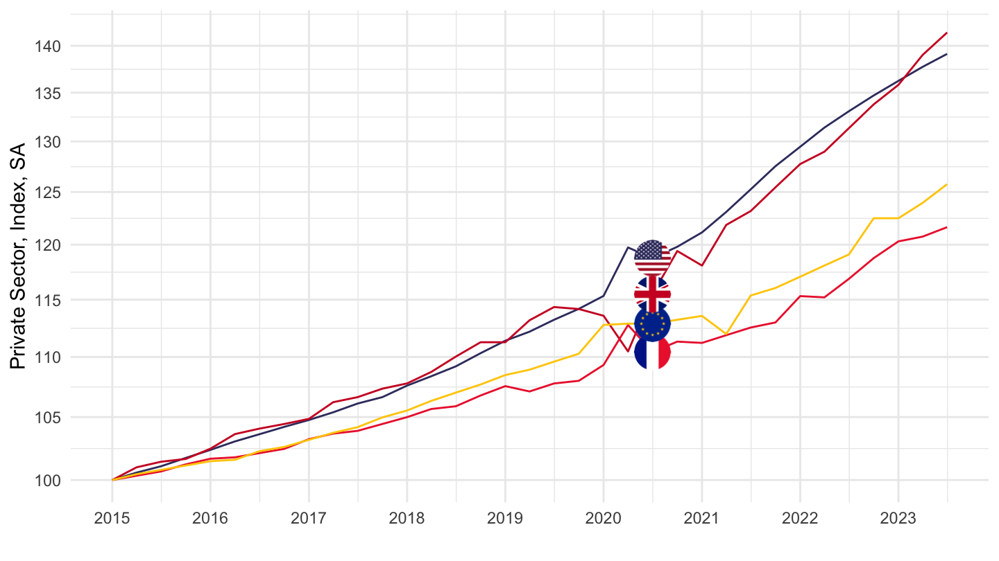
Real
Code
EAR_MEI %>%
  filter(SUBJECT == "LCEAPR_IXOBSA",
         FREQUENCY == "Q",
         LOCATION %in% c("USA", "EA19", "GBR", "FRA")) %>%
  quarter_to_date %>%
  filter(date >= as.Date("2015-01-01")) %>%
  left_join(EAR_MEI_var$LOCATION, by = "LOCATION") %>%
  left_join(PRICES_CPI_CPALTT01_IXOB, by = c("date", "Location", "LOCATION")) %>%
  mutate(Location = ifelse(LOCATION == "EA19", "Europe", Location)) %>%
  mutate(obsValue = obsValue/CPALTT01_IXOB) %>%
  left_join(colors, by = c("Location" = "country")) %>%
  mutate(color = ifelse(LOCATION == "EA19", color2, color)) %>%
  group_by(Location) %>%
  mutate(obsValue = 100*obsValue / obsValue[date == as.Date("2015-01-01")]) %>%
  ggplot(.) + geom_line(aes(x = date, y = obsValue, color = color)) +
  scale_color_identity() + theme_minimal() + add_4flags +
  scale_x_date(breaks = seq(1920, 2100, 1) %>% paste0("-01-01") %>% as.Date,
               labels = date_format("%Y")) +
  scale_y_log10(breaks = seq(10, 500, 1),
                     labels = scales::dollar_format(accuracy = 1, suffix = "", prefix = "")) +
  ylab("Private Sector, Index, SA, Real") + xlab("")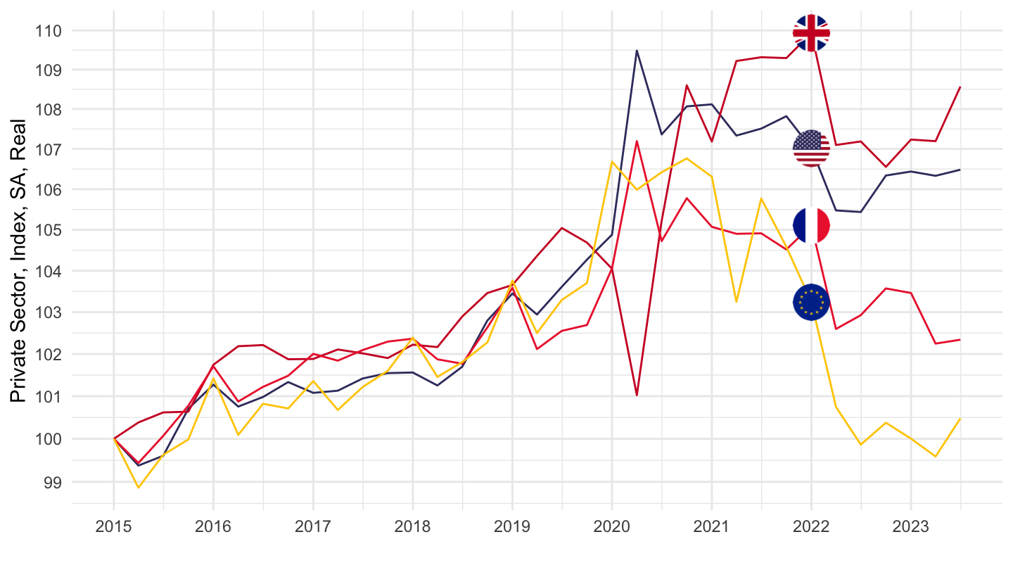
Eurozone, United States, United Kingdom, Germany
2015-
Nominal
Code
EAR_MEI %>%
  filter(SUBJECT == "LCEAPR_IXOBSA",
         FREQUENCY == "Q",
         LOCATION %in% c("USA", "EA19", "GBR", "DEU")) %>%
  quarter_to_date %>%
  filter(date >= as.Date("2015-01-01")) %>%
  left_join(EAR_MEI_var$LOCATION, by = "LOCATION") %>%
  mutate(Location = ifelse(LOCATION == "EA19", "Europe", Location)) %>%
  left_join(colors, by = c("Location" = "country")) %>%
  mutate(color = ifelse(LOCATION == "EA19", color2, color)) %>%
  group_by(Location) %>%
  mutate(obsValue = 100*obsValue / obsValue[date == as.Date("2015-01-01")]) %>%
  ggplot(.) + geom_line(aes(x = date, y = obsValue, color = color)) +
  scale_color_identity() + theme_minimal() + add_4flags +
  scale_x_date(breaks = seq(1920, 2100, 1) %>% paste0("-01-01") %>% as.Date,
               labels = date_format("%Y")) + add_6flags +
  scale_y_log10(breaks = seq(10, 500, 5),
                     labels = scales::dollar_format(accuracy = 1, suffix = "", prefix = "")) +
  ylab("Private Sector, Index, SA") + xlab("")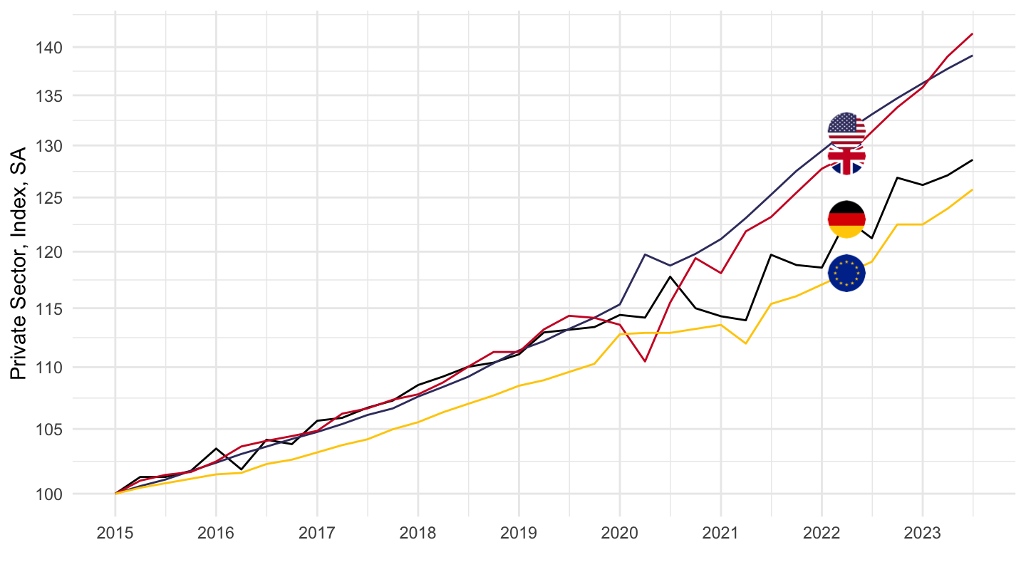
Real
Code
EAR_MEI %>%
  filter(SUBJECT == "LCEAPR_IXOBSA",
         FREQUENCY == "Q",
         LOCATION %in% c("USA", "EA19", "GBR", "DEU")) %>%
  quarter_to_date %>%
  filter(date >= as.Date("2015-01-01")) %>%
  left_join(EAR_MEI_var$LOCATION, by = "LOCATION") %>%
  left_join(PRICES_CPI_CPALTT01_IXOB, by = c("date", "Location", "LOCATION")) %>%
  mutate(Location = ifelse(LOCATION == "EA19", "Europe", Location)) %>%
  arrange(date) %>%
  mutate(obsValue = obsValue/CPALTT01_IXOB) %>%
  left_join(colors, by = c("Location" = "country")) %>%
  mutate(color = ifelse(LOCATION == "EA19", color2, color)) %>%
  group_by(Location) %>%
  mutate(obsValue = 100*obsValue / obsValue[date == as.Date("2015-01-01")]) %>%
  ggplot(.) + geom_line(aes(x = date, y = obsValue, color = color)) +
  scale_color_identity() + theme_minimal() + add_4flags +
  scale_x_date(breaks = seq(1920, 2100, 1) %>% paste0("-01-01") %>% as.Date,
               labels = date_format("%Y")) + add_6flags +
  scale_y_log10(breaks = seq(10, 500, 1),
                     labels = scales::dollar_format(accuracy = 1, suffix = "", prefix = "")) +
  ylab("Private Sector, Index, SA, Real") + xlab("")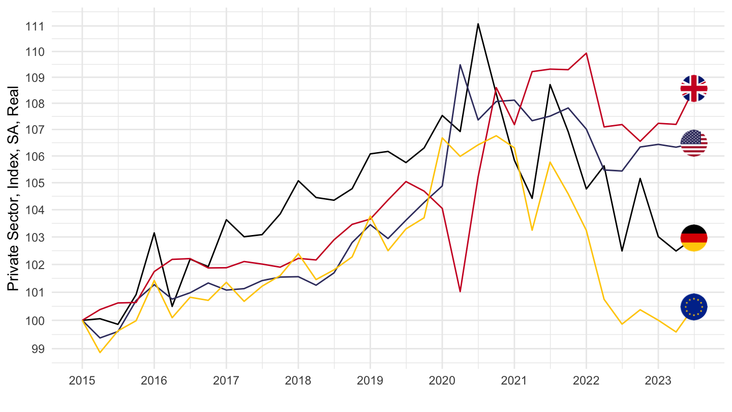
2021-
Code
df <- EAR_MEI %>%
  filter(SUBJECT == "LCEAPR_IXOBSA",
         FREQUENCY == "Q",
         LOCATION %in% c("USA", "EA19", "GBR", "DEU")) %>%
  quarter_to_date %>%
  filter(date >= as.Date("2021-01-01")) %>%
  left_join(EAR_MEI_var$LOCATION, by = "LOCATION") %>%
  left_join(PRICES_CPI_CPALTT01_IXOB, by = c("date", "Location", "LOCATION")) %>%
  mutate(Location = ifelse(LOCATION == "EA19", "Europe", Location)) %>%
  arrange(date) %>%
  mutate(obsValue = obsValue/CPALTT01_IXOB) %>%
  left_join(colors, by = c("Location" = "country")) %>%
  mutate(color = ifelse(LOCATION == "EA19", color2, color)) %>%
  group_by(Location) %>%
  mutate(obsValue = 100*obsValue / obsValue[date == as.Date("2021-01-01")]) %>%
  mutate(date = zoo::as.yearqtr(paste0(year(date), " Q", quarter(date))))

  ggplot(data = df) + geom_line(aes(x = date, y = obsValue, color = color)) +
  scale_color_identity() + theme_minimal() + add_4flags +
  theme(axis.text.x = element_text(angle = 45, vjust = 1, hjust = 1)) +
  scale_x_yearqtr(labels = date_format("%Y Q%q"),
                  breaks = seq(from = min(df$date), to = max(df$date), by = 0.25)) +
  scale_y_log10(breaks = seq(10, 500, 1),
                     labels = scales::dollar_format(accuracy = 1, suffix = "", prefix = "")) +
  ylab("Private Sector, Index, SA, Real") + xlab("")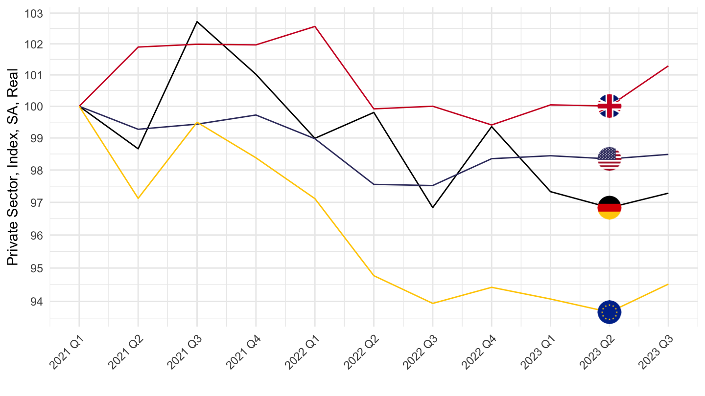
US, Eurozone, Germany, France
2019Q4-
Code
df <- EAR_MEI %>%
  filter(SUBJECT == "LCEAPR_IXOBSA",
         FREQUENCY == "Q",
         LOCATION %in% c("USA", "EA19", "DEU", "FRA")) %>%
  quarter_to_date %>%
  filter(date >= as.Date("2019-10-01")) %>%
  left_join(EAR_MEI_var$LOCATION, by = "LOCATION") %>%
  left_join(PRICES_CPI_CPALTT01_IXOB, by = c("date", "Location", "LOCATION")) %>%
  mutate(Location = ifelse(LOCATION == "EA19", "Europe", Location)) %>%
  arrange(date) %>%
  mutate(obsValue = obsValue/CPALTT01_IXOB) %>%
  left_join(colors, by = c("Location" = "country")) %>%
  mutate(color = ifelse(LOCATION == "EA19", color2, color)) %>%
  group_by(Location) %>%
  mutate(obsValue = 100*obsValue / obsValue[date == as.Date("2019-10-01")]) %>%
  mutate(date = zoo::as.yearqtr(paste0(year(date), " Q", quarter(date))))

  ggplot(data = df) + geom_line(aes(x = date, y = obsValue, color = color)) +
  scale_color_identity() + theme_minimal() + add_4flags +
  theme(axis.text.x = element_text(angle = 45, vjust = 1, hjust = 1)) +
  scale_x_yearqtr(labels = date_format("%Y Q%q"),
                  breaks = seq(from = min(df$date), to = max(df$date), by = 0.25)) +
  scale_y_log10(breaks = seq(10, 500, 1),
                     labels = scales::dollar_format(accuracy = 1, suffix = "", prefix = "")) +
  ylab("Private Sector, Index, SA, Real") + xlab("")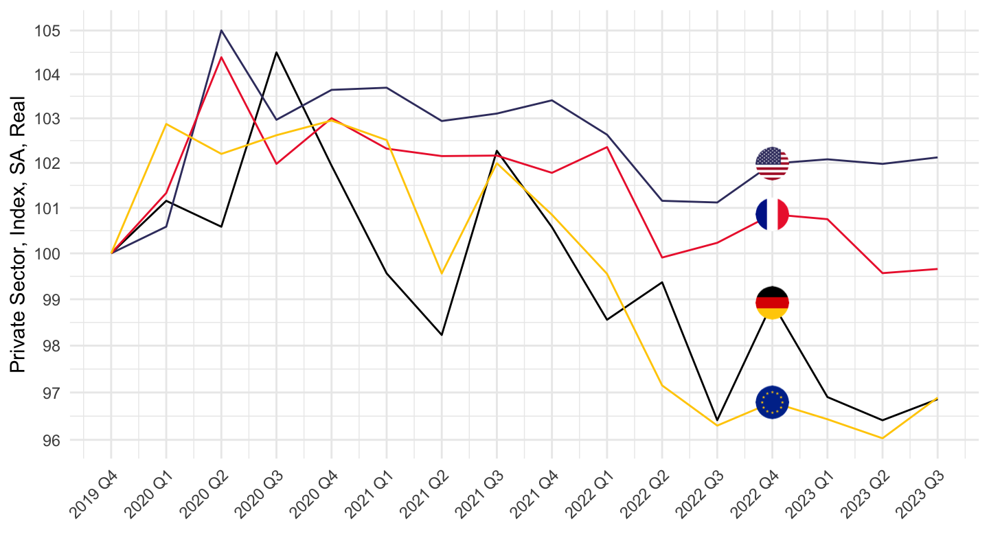
2017-
Code
df <- EAR_MEI %>%
  filter(SUBJECT == "LCEAPR_IXOBSA",
         FREQUENCY == "Q",
         LOCATION %in% c("USA", "EA19", "DEU", "FRA")) %>%
  quarter_to_date %>%
  filter(date >= as.Date("2017-01-01")) %>%
  left_join(EAR_MEI_var$LOCATION, by = "LOCATION") %>%
  left_join(PRICES_CPI_CPALTT01_IXOB, by = c("date", "Location", "LOCATION")) %>%
  mutate(Location = ifelse(LOCATION == "EA19", "Europe", Location)) %>%
  arrange(date) %>%
  mutate(obsValue = obsValue/CPALTT01_IXOB) %>%
  left_join(colors, by = c("Location" = "country")) %>%
  mutate(color = ifelse(LOCATION == "EA19", color2, color)) %>%
  group_by(Location) %>%
  mutate(obsValue = 100*obsValue / obsValue[date == as.Date("2017-01-01")]) %>%
  mutate(date = zoo::as.yearqtr(paste0(year(date), " Q", quarter(date))))

  ggplot(data = df) + geom_line(aes(x = date, y = obsValue, color = color)) +
  scale_color_identity() + theme_minimal() + add_4flags +
  theme(axis.text.x = element_text(angle = 45, vjust = 1, hjust = 1)) +
  scale_x_yearqtr(labels = date_format("%Y Q%q"),
                  breaks = seq(from = min(df$date), to = max(df$date), by = 0.25)) +
  scale_y_log10(breaks = seq(10, 500, 1),
                     labels = scales::dollar_format(accuracy = 1, suffix = "", prefix = "")) +
  ylab("Private Sector, Index, SA, Real") + xlab("")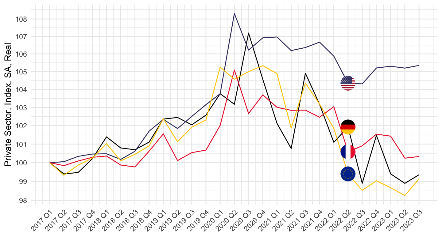
2019-
Code
df <- EAR_MEI %>%
  filter(SUBJECT == "LCEAPR_IXOBSA",
         FREQUENCY == "Q",
         LOCATION %in% c("USA", "EA19", "DEU", "FRA")) %>%
  quarter_to_date %>%
  filter(date >= as.Date("2019-01-01")) %>%
  left_join(EAR_MEI_var$LOCATION, by = "LOCATION") %>%
  left_join(PRICES_CPI_CPALTT01_IXOB, by = c("date", "Location", "LOCATION")) %>%
  mutate(Location = ifelse(LOCATION == "EA19", "Europe", Location)) %>%
  arrange(date) %>%
  mutate(obsValue = obsValue/CPALTT01_IXOB) %>%
  left_join(colors, by = c("Location" = "country")) %>%
  mutate(color = ifelse(LOCATION == "EA19", color2, color)) %>%
  group_by(Location) %>%
  mutate(obsValue = 100*obsValue / obsValue[date == as.Date("2019-01-01")]) %>%
  mutate(date = zoo::as.yearqtr(paste0(year(date), " Q", quarter(date))))

  ggplot(data = df) + geom_line(aes(x = date, y = obsValue, color = color)) +
  scale_color_identity() + theme_minimal() + add_4flags +
  theme(axis.text.x = element_text(angle = 45, vjust = 1, hjust = 1)) +
  scale_x_yearqtr(labels = date_format("%Y Q%q"),
                  breaks = seq(from = min(df$date), to = max(df$date), by = 0.25)) +
  scale_y_log10(breaks = seq(10, 500, 1),
                     labels = scales::dollar_format(accuracy = 1, suffix = "", prefix = "")) +
  ylab("Private Sector, Index, SA, Real") + xlab("")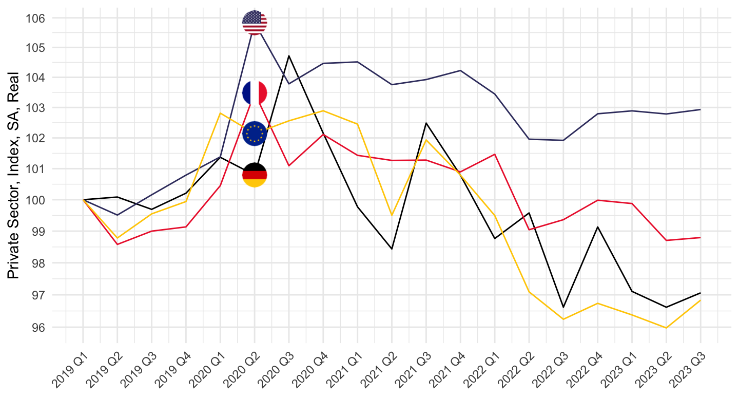
2021-
Code
df <- EAR_MEI %>%
  filter(SUBJECT == "LCEAPR_IXOBSA",
         FREQUENCY == "Q",
         LOCATION %in% c("USA", "EA19", "DEU", "FRA")) %>%
  quarter_to_date %>%
  filter(date >= as.Date("2021-01-01")) %>%
  left_join(EAR_MEI_var$LOCATION, by = "LOCATION") %>%
  left_join(PRICES_CPI_CPALTT01_IXOB, by = c("date", "Location", "LOCATION")) %>%
  mutate(Location = ifelse(LOCATION == "EA19", "Europe", Location)) %>%
  arrange(date) %>%
  mutate(obsValue = obsValue/CPALTT01_IXOB) %>%
  left_join(colors, by = c("Location" = "country")) %>%
  mutate(color = ifelse(LOCATION == "EA19", color2, color)) %>%
  group_by(Location) %>%
  mutate(obsValue = 100*obsValue / obsValue[date == as.Date("2021-01-01")]) %>%
  mutate(date = zoo::as.yearqtr(paste0(year(date), " Q", quarter(date))))

  ggplot(data = df) + geom_line(aes(x = date, y = obsValue, color = color)) +
  scale_color_identity() + theme_minimal() + add_4flags +
  theme(axis.text.x = element_text(angle = 45, vjust = 1, hjust = 1)) +
  scale_x_yearqtr(labels = date_format("%Y Q%q"),
                  breaks = seq(from = min(df$date), to = max(df$date), by = 0.25)) +
  scale_y_log10(breaks = seq(10, 500, 1),
                     labels = scales::dollar_format(accuracy = 1, suffix = "", prefix = "")) +
  ylab("Private Sector, Index, SA, Real") + xlab("")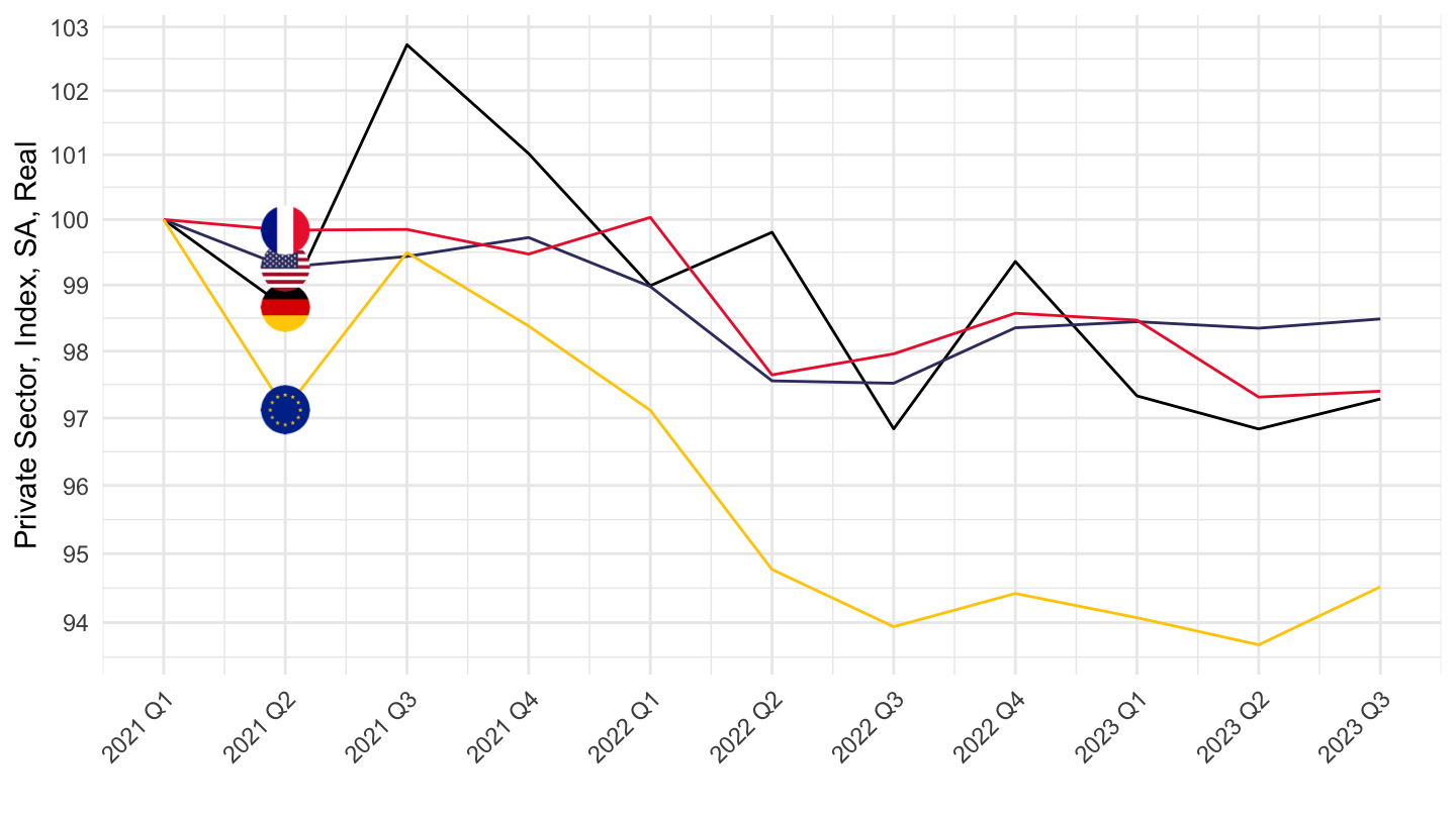
Manufacturing, Index, SA
Table
Code
EAR_MEI %>%
  filter(SUBJECT == "LCEAMN01_IXOBSA") %>%
  left_join(EAR_MEI_var$LOCATION, by = "LOCATION") %>%
  group_by(LOCATION, Location) %>%
  summarise(Nobs = n()) %>%
  arrange(-Nobs) %>%
  mutate(Flag = gsub(" ", "-", str_to_lower(gsub(" ", "-", Location))),
         Flag = paste0('<img src="../../icon/flag/vsmall/', Flag, '.png" alt="Flag">')) %>%
  select(Flag, everything()) %>%
  {if (is_html_output()) datatable(., filter = 'top', rownames = F, escape = F) else .}
U.S., Europe, U.K., Germany
Code
EAR_MEI %>%
  filter(SUBJECT == "LCEAMN01_IXOBSA",
         FREQUENCY == "Q",
         LOCATION %in% c("USA", "EA19", "GBR", "DEU")) %>%
  quarter_to_date %>%
  filter(date >= as.Date("2015-01-01")) %>%
  left_join(EAR_MEI_var$LOCATION, by = "LOCATION") %>%
  left_join(PRICES_CPI_CPALTT01_IXOB, by = c("date", "Location", "LOCATION")) %>%
  mutate(Location = ifelse(LOCATION == "EA19", "Europe", Location)) %>%
  mutate(obsValue = obsValue/CPALTT01_IXOB) %>%
  left_join(colors, by = c("Location" = "country")) %>%
  mutate(color = ifelse(LOCATION == "EA19", color2, color)) %>%
  group_by(Location) %>%
  mutate(obsValue = 100*obsValue / obsValue[date == as.Date("2015-01-01")]) %>%
  ggplot(.) + geom_line(aes(x = date, y = obsValue, color = color)) +
  scale_color_identity() + theme_minimal() + add_4flags +
  scale_x_date(breaks = seq(1920, 2100, 1) %>% paste0("-01-01") %>% as.Date,
               labels = date_format("%Y")) + add_6flags +
  scale_y_log10(breaks = seq(10, 500, 1),
                     labels = scales::dollar_format(accuracy = 1, suffix = "", prefix = "")) +
  ylab("Manufacturing Sector, Index, SA, Real") + xlab("")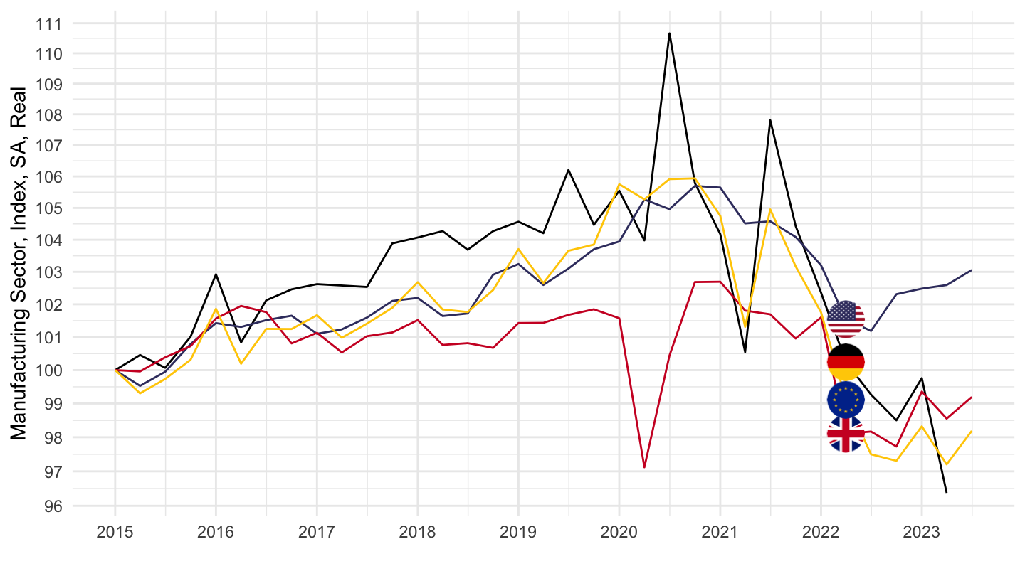
U.S., Europe, U.K., Germany, France
2015-
Code
EAR_MEI %>%
  filter(SUBJECT == "LCEAMN01_IXOBSA",
         FREQUENCY == "Q",
         LOCATION %in% c("USA", "EA19", "GBR", "DEU", "FRA")) %>%
  quarter_to_date %>%
  filter(date >= as.Date("2015-01-01")) %>%
  left_join(EAR_MEI_var$LOCATION, by = "LOCATION") %>%
  left_join(PRICES_CPI_CPALTT01_IXOB, by = c("date", "Location", "LOCATION")) %>%
  mutate(Location = ifelse(LOCATION == "EA19", "Europe", Location)) %>%
  mutate(obsValue = obsValue/CPALTT01_IXOB) %>%
  left_join(colors, by = c("Location" = "country")) %>%
  mutate(color = ifelse(LOCATION == "EA19", color2, color)) %>%
  group_by(Location) %>%
  mutate(obsValue = 100*obsValue / obsValue[date == as.Date("2015-01-01")]) %>%
  ggplot(.) + geom_line(aes(x = date, y = obsValue, color = color)) +
  scale_color_identity() + theme_minimal() + add_5flags +
  scale_x_date(breaks = seq(1920, 2100, 1) %>% paste0("-01-01") %>% as.Date,
               labels = date_format("%Y")) + add_6flags +
  scale_y_log10(breaks = seq(10, 500, 1),
                     labels = scales::dollar_format(accuracy = 1, suffix = "", prefix = "")) +
  ylab("Manufacturing Sector, Index, SA, Real") + xlab("")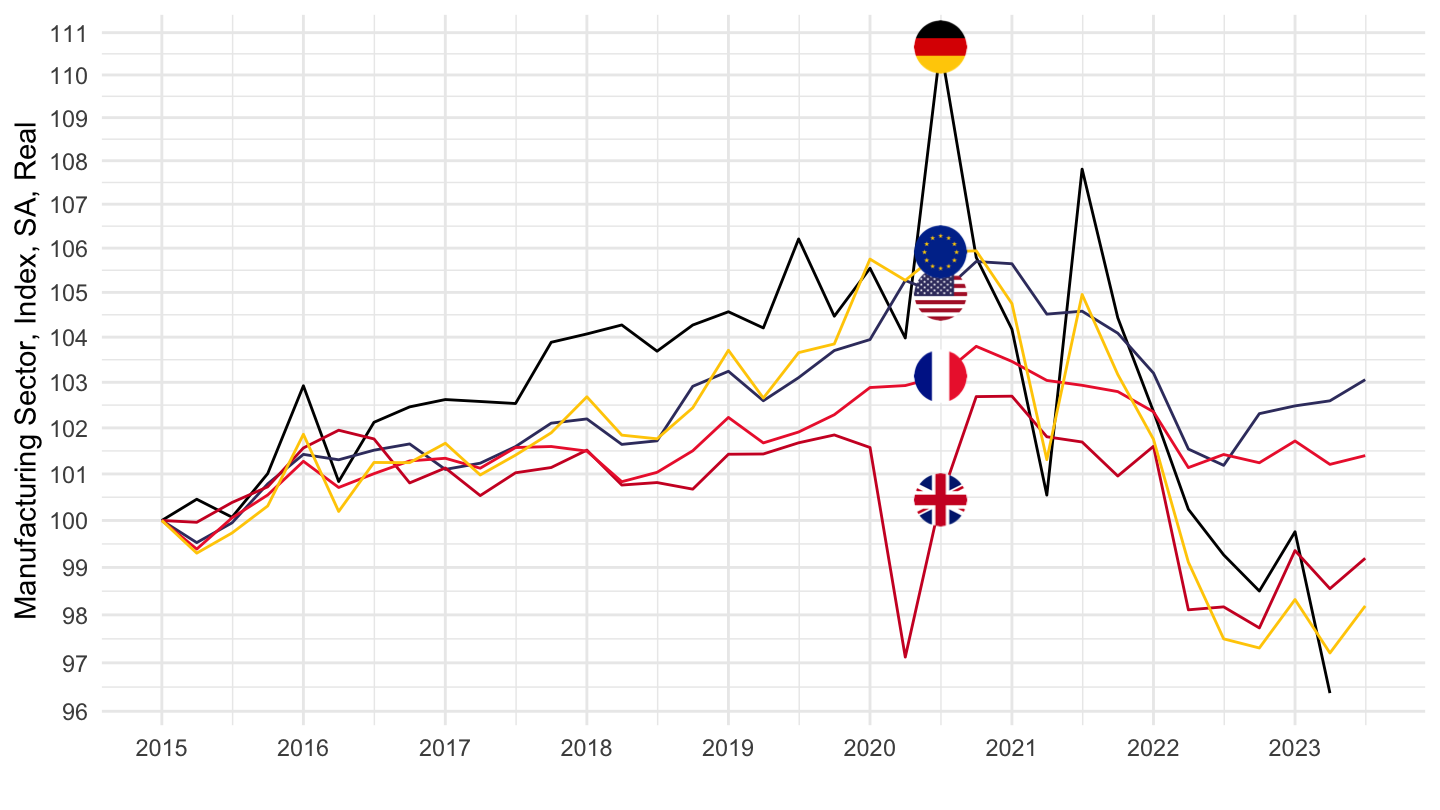
2019-Q4-
Code
df <- EAR_MEI %>%
  filter(SUBJECT == "LCEAMN01_IXOBSA",
         FREQUENCY == "Q",
         LOCATION %in% c("USA", "EA19", "GBR", "DEU", "FRA")) %>%
  quarter_to_date %>%
  filter(date >= as.Date("2019-10-01")) %>%
  left_join(EAR_MEI_var$LOCATION, by = "LOCATION") %>%
  left_join(PRICES_CPI_CPALTT01_IXOB, by = c("date", "Location", "LOCATION")) %>%
  mutate(Location = ifelse(LOCATION == "EA19", "Europe", Location)) %>%
  mutate(obsValue = obsValue/CPALTT01_IXOB) %>%
  left_join(colors, by = c("Location" = "country")) %>%
  mutate(color = ifelse(LOCATION == "EA19", color2, color)) %>%
  group_by(Location) %>%
  mutate(obsValue = 100*obsValue / obsValue[date == as.Date("2019-10-01")]) %>%
  mutate(date = zoo::as.yearqtr(paste0(year(date), " Q", quarter(date))))

  ggplot(data = df) + geom_line(aes(x = date, y = obsValue, color = color)) +
  scale_color_identity() + theme_minimal() + add_5flags +
  theme(axis.text.x = element_text(angle = 45, vjust = 1, hjust = 1)) +
  scale_x_yearqtr(labels = date_format("%Y Q%q"),
                  breaks = seq(from = min(df$date), to = max(df$date), by = 0.25)) +
  add_6flags +
  scale_y_log10(breaks = seq(10, 500, 1),
                     labels = scales::dollar_format(accuracy = 1, suffix = "", prefix = "")) +
  ylab("Manufacturing Sector, Index, SA, Real") + xlab("")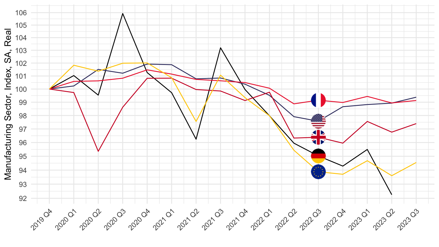
Plus Italy, Spain, etc.
2019-Q4-
Code
df <- EAR_MEI %>%
  filter(SUBJECT == "LCEAMN01_IXOBSA",
         FREQUENCY == "Q",
         LOCATION %in% c("USA", "EA19", "GBR", "DEU", "FRA", "ITA", "ESP")) %>%
  quarter_to_date %>%
  filter(date >= as.Date("2019-10-01")) %>%
  left_join(EAR_MEI_var$LOCATION, by = "LOCATION") %>%
  left_join(PRICES_CPI_CPALTT01_IXOB, by = c("date", "Location", "LOCATION")) %>%
  mutate(Location = ifelse(LOCATION == "EA19", "Europe", Location)) %>%
  mutate(obsValue = obsValue/CPALTT01_IXOB) %>%
  left_join(colors, by = c("Location" = "country")) %>%
  mutate(color = ifelse(LOCATION == "EA19", color2, color)) %>%
  group_by(Location) %>%
  mutate(obsValue = 100*obsValue / obsValue[date == as.Date("2019-10-01")]) %>%
  mutate(date = zoo::as.yearqtr(paste0(year(date), " Q", quarter(date))))

ggplot(data = df) + geom_line(aes(x = date, y = obsValue, color = color)) +
  scale_color_identity() + theme_minimal() + add_7flags + add_6flags +
  theme(axis.text.x = element_text(angle = 45, vjust = 1, hjust = 1)) +
  scale_x_yearqtr(labels = date_format("%Y Q%q"),
                  breaks = seq(from = min(df$date), to = max(df$date), by = 0.25)) +
  scale_y_log10(breaks = seq(10, 500, 1),
                     labels = scales::dollar_format(accuracy = 1, suffix = "", prefix = "")) +
  ylab("Manufacturing Sector, Index, SA, Real") + xlab("")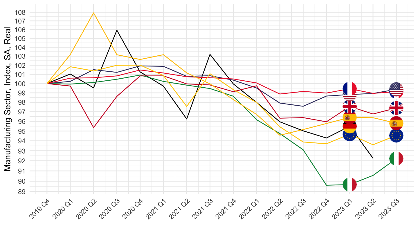
Germany, Italy, Netherlands, Spain, France
2019-Q4-
Code
df <- EAR_MEI %>%
  filter(SUBJECT == "LCEAMN01_IXOBSA",
         FREQUENCY == "Q",
         LOCATION %in% c("DEU", "ITA", "NLD", "ESP", "FRA")) %>%
  quarter_to_date %>%
  filter(date >= as.Date("2019-10-01")) %>%
  left_join(EAR_MEI_var$LOCATION, by = "LOCATION") %>%
  left_join(PRICES_CPI_CPALTT01_IXOB, by = c("date", "Location", "LOCATION")) %>%
  mutate(Location = ifelse(LOCATION == "EA19", "Europe", Location)) %>%
  mutate(obsValue = obsValue/CPALTT01_IXOB) %>%
  left_join(colors, by = c("Location" = "country")) %>%
  mutate(color = ifelse(LOCATION == "EA19", color2, color)) %>%
  group_by(Location) %>%
  mutate(obsValue = 100*obsValue / obsValue[date == as.Date("2019-10-01")]) %>%
  mutate(date = zoo::as.yearqtr(paste0(year(date), " Q", quarter(date))))

ggplot(data = df) + geom_line(aes(x = date, y = obsValue, color = color)) +
  scale_color_identity() + theme_minimal() + add_5flags +
  theme(axis.text.x = element_text(angle = 45, vjust = 1, hjust = 1)) +
  scale_x_yearqtr(labels = date_format("%Y Q%q"),
                  breaks = seq(from = min(df$date), to = max(df$date), by = 0.25)) +
  add_6flags +
  scale_y_log10(breaks = seq(10, 500, 1),
                     labels = scales::dollar_format(accuracy = 1, suffix = "", prefix = "")) +
  ylab("Manufacturing Sector, Index, SA, Real") + xlab("")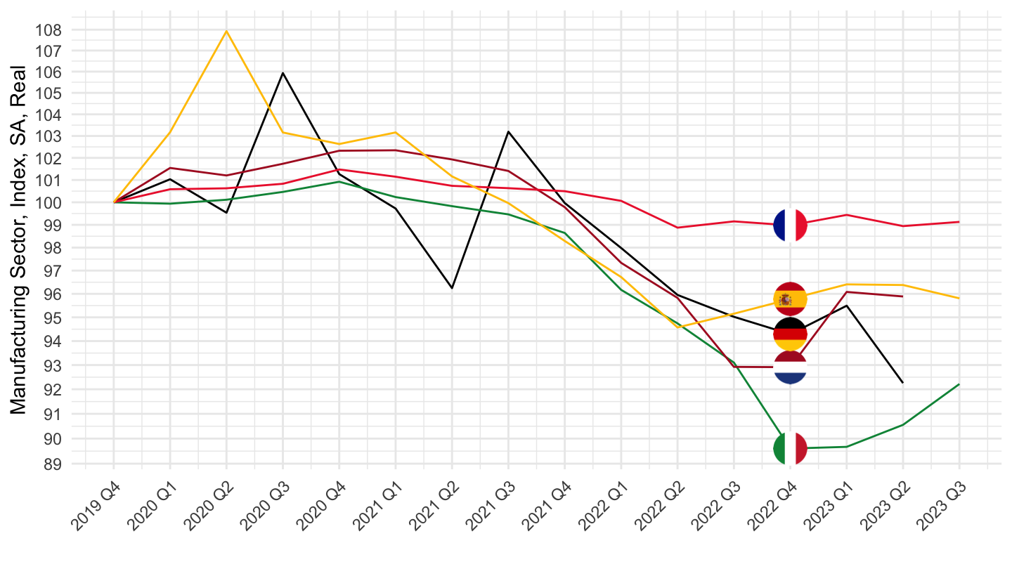
Germany, Italy, Netherlands, Spain, France
2019-Q4-
Code
df <- EAR_MEI %>%
  filter(SUBJECT == "LCEAMN01_IXOBSA",
         FREQUENCY == "Q",
         LOCATION %in% c("DEU", "ITA", "NLD", "ESP", "FRA")) %>%
  quarter_to_date %>%
  filter(date >= as.Date("2019-10-01")) %>%
  left_join(EAR_MEI_var$LOCATION, by = "LOCATION") %>%
  left_join(PRICES_CPI_CPALTT01_IXOB, by = c("date", "Location", "LOCATION")) %>%
  mutate(Location = ifelse(LOCATION == "EA19", "Europe", Location)) %>%
  mutate(obsValue = obsValue/CPALTT01_IXOB) %>%
  left_join(colors, by = c("Location" = "country")) %>%
  mutate(color = ifelse(LOCATION == "EA19", color2, color)) %>%
  group_by(Location) %>%
  mutate(obsValue = 100*obsValue / obsValue[date == as.Date("2019-10-01")]) %>%
  mutate(date = zoo::as.yearqtr(paste0(year(date), " Q", quarter(date))))

ggplot(data = df) + geom_line(aes(x = date, y = obsValue, color = color)) +
  scale_color_identity() + theme_minimal() +
  add_5flags +
  theme(axis.text.x = element_text(angle = 45, vjust = 1, hjust = 1)) +
  scale_x_yearqtr(labels = date_format("%Y Q%q"),
                  breaks = seq(from = min(df$date), to = max(df$date), by = 0.25)) +
  add_6flags +
  scale_y_log10(breaks = seq(10, 500, 1),
                     labels = scales::dollar_format(accuracy = 1, suffix = "", prefix = "")) +
  ylab("Manufacturing Sector, Index, SA, Real") + xlab("")
United States, Euro, UK
Code
df <- EAR_MEI %>%
  filter(SUBJECT == "LCEAMN01_IXOBSA",
         FREQUENCY == "Q",
         LOCATION %in% c("USA", "EA19", "GBR")) %>%
  quarter_to_date %>%
  filter(date >= as.Date("2015-01-01")) %>%
  left_join(EAR_MEI_var$LOCATION, by = "LOCATION") %>%
  left_join(PRICES_CPI_CPALTT01_IXOB, by = c("date", "Location", "LOCATION")) %>%
  mutate(Location = ifelse(LOCATION == "EA19", "Europe", Location)) %>%
  mutate(obsValue = obsValue/CPALTT01_IXOB) %>%
  left_join(colors, by = c("Location" = "country")) %>%
  mutate(color = ifelse(LOCATION == "EA19", color2, color)) %>%
  group_by(Location) %>%
  mutate(obsValue = 100*obsValue / obsValue[date == as.Date("2015-01-01")]) %>%
  mutate(date = zoo::as.yearqtr(paste0(year(date), " Q", quarter(date))))


ggplot(data = df) + geom_line(aes(x = date, y = obsValue, color = color)) +
  scale_color_identity() + theme_minimal() + add_3flags +
  theme(axis.text.x = element_text(angle = 45, vjust = 1, hjust = 1)) +
  scale_x_yearqtr(labels = date_format("%Y Q%q"),
                  breaks = seq(from = min(df$date), to = max(df$date), by = 0.25)) +
  add_6flags +
  scale_y_log10(breaks = seq(10, 500, 1),
                     labels = scales::dollar_format(accuracy = 1, suffix = "", prefix = "")) +
  ylab("Manufacturing Sector, Index, SA, Real") + xlab("")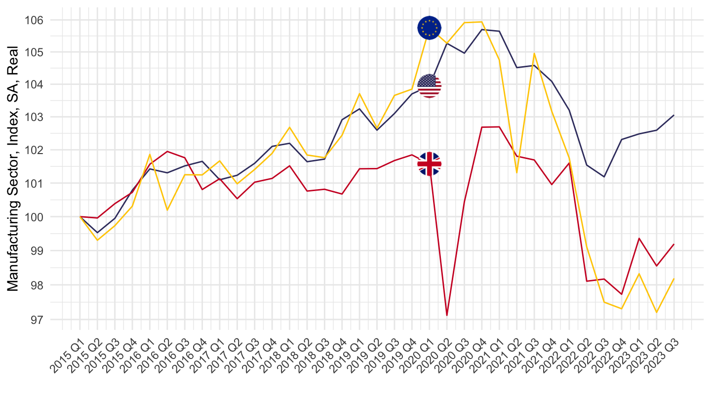
United States, Euro, UK
2015-
Code
df <- EAR_MEI %>%
  filter(SUBJECT == "LCEAMN01_IXOBSA",
         FREQUENCY == "Q",
         LOCATION %in% c("USA", "EA19")) %>%
  quarter_to_date %>%
  filter(date >= as.Date("2015-01-01")) %>%
  left_join(EAR_MEI_var$LOCATION, by = "LOCATION") %>%
  left_join(PRICES_CPI_CPALTT01_IXOB, by = c("date", "Location", "LOCATION")) %>%
  mutate(Location = ifelse(LOCATION == "EA19", "Europe", Location)) %>%
  mutate(obsValue = obsValue/CPALTT01_IXOB) %>%
  left_join(colors, by = c("Location" = "country")) %>%
  mutate(color = ifelse(LOCATION == "EA19", color2, color)) %>%
  group_by(Location) %>%
  mutate(obsValue = 100*obsValue / obsValue[date == as.Date("2015-01-01")]) %>%
  mutate(date = zoo::as.yearqtr(paste0(year(date), " Q", quarter(date))))


ggplot(data = df) + geom_line(aes(x = date, y = obsValue, color = color)) +
  scale_color_identity() + theme_minimal() + add_2flags +
  theme(axis.text.x = element_text(angle = 45, vjust = 1, hjust = 1)) +
  scale_x_yearqtr(labels = date_format("%Y Q%q"),
                  breaks = seq(from = min(df$date), to = max(df$date), by = 0.25)) +
  add_6flags +
  scale_y_log10(breaks = seq(10, 500, 1),
                     labels = scales::dollar_format(accuracy = 1, suffix = "", prefix = "")) +
  ylab("Manufacturing Sector, Index, SA, Real") + xlab("")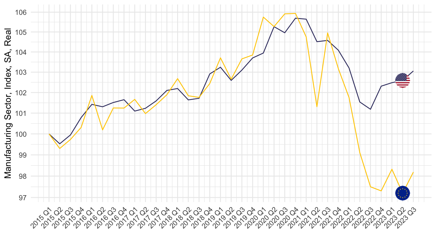
2017-
Code
df <- EAR_MEI %>%
  filter(SUBJECT == "LCEAMN01_IXOBSA",
         FREQUENCY == "Q",
         LOCATION %in% c("USA", "EA19")) %>%
  quarter_to_date %>%
  filter(date >= as.Date("2017-01-01")) %>%
  left_join(EAR_MEI_var$LOCATION, by = "LOCATION") %>%
  left_join(PRICES_CPI_CPALTT01_IXOB, by = c("date", "Location", "LOCATION")) %>%
  mutate(Location = ifelse(LOCATION == "EA19", "Europe", Location)) %>%
  mutate(obsValue = obsValue/CPALTT01_IXOB) %>%
  left_join(colors, by = c("Location" = "country")) %>%
  mutate(color = ifelse(LOCATION == "EA19", color2, color)) %>%
  group_by(Location) %>%
  mutate(obsValue = 100*obsValue / obsValue[date == as.Date("2017-01-01")]) %>%
  mutate(date = zoo::as.yearqtr(paste0(year(date), " Q", quarter(date))))


ggplot(data = df) + geom_line(aes(x = date, y = obsValue, color = color)) +
  scale_color_identity() + theme_minimal() + add_2flags +
  theme(axis.text.x = element_text(angle = 45, vjust = 1, hjust = 1)) +
  scale_x_yearqtr(labels = date_format("%Y Q%q"),
                  breaks = seq(from = min(df$date), to = max(df$date), by = 0.25)) +
  add_6flags +
  scale_y_log10(breaks = seq(10, 500, 1),
                     labels = scales::dollar_format(accuracy = 1, suffix = "", prefix = "")) +
  ylab("Manufacturing Sector, Index, SA, Real") + xlab("")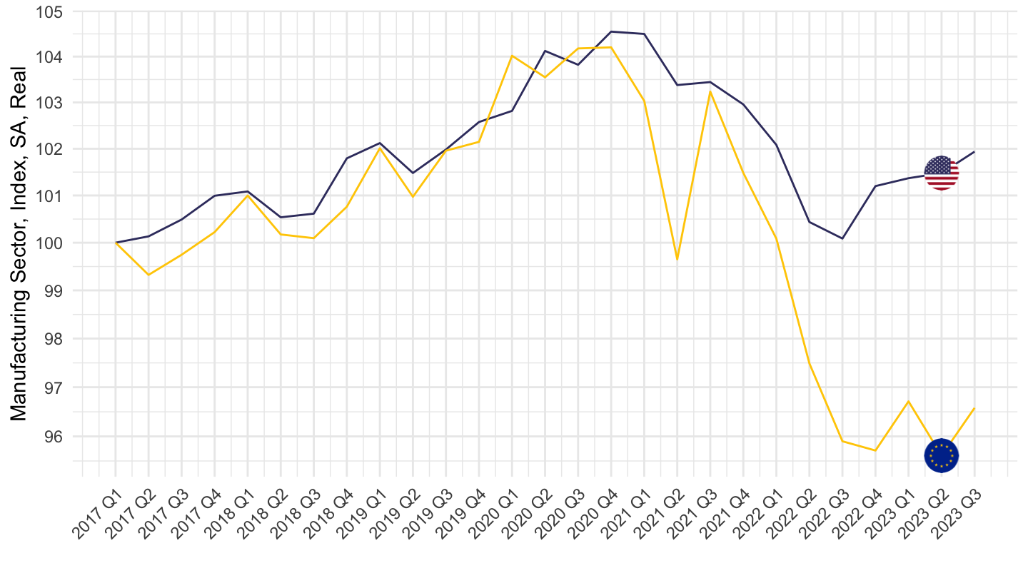
Switzerland, Australia, Mexico
Code
EAR_MEI %>%
  filter(SUBJECT == "LCEAMN01_IXOBSA",
         FREQUENCY == "A",
         LOCATION %in% c("AUS", "MEX", "CHE")) %>%
  left_join(EAR_MEI_var$LOCATION, by = "LOCATION") %>%
  year_to_date %>%
  left_join(colors, by = c("Location" = "country")) %>%
  ggplot(.) + geom_line(aes(x = date, y = obsValue, color = color)) +
  scale_color_identity() + theme_minimal() +
  scale_x_date(breaks = seq(1920, 2100, 5) %>% paste0("-01-01") %>% as.Date,
               labels = date_format("%Y")) +
  scale_y_log10(breaks = seq(10, 500, 10),
                     labels = scales::dollar_format(accuracy = 1, suffix = " k", prefix = "")) +
  ylab("Manufacturing, Index, SA") + xlab("")