Short-Term Statistics - STS
Data - ECB
Info
Data on wages
| source | dataset | Title | .html | .rData |
|---|---|---|---|---|
| eurostat | earn_mw_cur | Monthly minimum wages - bi-annual data | 2026-07-23 | 2026-07-23 |
| eurostat | ei_lmlc_q | Labour cost index, nominal value - quarterly data | 2026-07-23 | 2026-07-23 |
| eurostat | lc_lci_lev | Labour cost levels by NACE Rev. 2 activity | 2026-07-24 | 2026-07-24 |
| eurostat | lc_lci_r2_q | Labour cost index by NACE Rev. 2 activity - nominal value, quarterly data | 2026-07-24 | 2026-07-23 |
| eurostat | nama_10_lp_ulc | Labour productivity and unit labour costs | 2026-07-22 | 2026-07-23 |
| eurostat | namq_10_lp_ulc | Labour productivity and unit labour costs | 2026-07-24 | 2026-07-24 |
| eurostat | tps00155 | Minimum wages | 2026-07-24 | 2026-07-23 |
| fred | wage | Wage | 2026-07-24 | 2026-07-24 |
| ilo | EAR_4MTH_SEX_ECO_CUR_NB_A | Mean nominal monthly earnings of employees by sex and economic activity -- Harmonized series | 2026-07-25 | 2023-06-01 |
| ilo | EAR_XEES_SEX_ECO_NB_Q | Mean nominal monthly earnings of employees by sex and economic activity -- Harmonized series | 2026-07-25 | 2023-06-01 |
| oecd | AV_AN_WAGE | Average annual wages | 2026-07-24 | 2026-07-24 |
| oecd | AWCOMP | Taxing Wages - Comparative tables | 2026-07-24 | 2023-09-09 |
| oecd | EAR_MEI | Hourly Earnings (MEI) | 2026-07-24 | 2024-04-16 |
| oecd | HH_DASH | Household Dashboard | 2026-07-24 | 2023-09-09 |
| oecd | MIN2AVE | Minimum relative to average wages of full-time workers - MIN2AVE | 2026-02-22 | 2023-09-09 |
| oecd | RMW | Real Minimum Wages - RMW | 2026-07-24 | 2024-03-12 |
| oecd | ULC_EEQ | Unit labour costs and labour productivity (employment based), Total economy | 2026-07-24 | 2024-04-15 |
LAST_DOWNLOAD
| LAST_DOWNLOAD |
|---|
| 2025-08-28 |
LAST_COMPILE
| LAST_COMPILE |
|---|
| 2026-07-26 |
Last
Code
STS %>%
  group_by(TIME_PERIOD) %>%
  summarise(Nobs = n()) %>%
  arrange(desc(TIME_PERIOD)) %>%
  head(1) %>%
print_table_conditional()| TIME_PERIOD | Nobs |
|---|---|
| 2025-Q3 | 50 |
STS_CONCEPT
All
Code
STS %>%
  left_join(STS_CONCEPT,  by = "STS_CONCEPT") %>%
  group_by(STS_CONCEPT, Sts_concept) %>%
  summarise(Nobs = n()) %>%
  {if (is_html_output()) datatable(., filter = 'top', rownames = F) else .}
Monthly
Code
STS %>%
  filter(FREQ == "M") %>%
  left_join(STS_CONCEPT,  by = "STS_CONCEPT") %>%
  group_by(STS_CONCEPT, Sts_concept) %>%
  summarise(Nobs = n()) %>%
  {if (is_html_output()) datatable(., filter = 'top', rownames = F) else .}
STS_CLASS
Code
STS %>%
  left_join(STS_CLASS,  by = "STS_CLASS") %>%
  group_by(STS_CLASS, Sts_class) %>%
  summarise(Nobs = n()) %>%
  arrange(-Nobs) %>%
  {if (is_html_output()) datatable(., filter = 'top', rownames = F) else .}
TITLE
All
Code
STS %>%
  group_by(TITLE) %>%
  summarise(Nobs = n()) %>%
  arrange(-Nobs) %>%
  {if (is_html_output()) datatable(., filter = 'top', rownames = F) else .}
Monthly
Code
STS %>%
  filter(FREQ == "M") %>%
  group_by(TITLE) %>%
  summarise(Nobs = n()) %>%
  {if (is_html_output()) datatable(., filter = 'top', rownames = F) else .}
ADJUSTMENT
Code
STS %>%
  left_join(ADJUSTMENT,  by = "ADJUSTMENT") %>%
  group_by(ADJUSTMENT, Adjustment) %>%
  summarise(Nobs = n()) %>%
  arrange(-Nobs) %>%
print_table_conditional()| ADJUSTMENT | Adjustment | Nobs |
|---|---|---|
| N | Neither seasonally nor working day adjusted | 667660 |
| W | Working day adjusted, not seasonally adjusted | 432610 |
| Y | Working day and seasonally adjusted | 427234 |
| S | Seasonally adjusted, not working day adjusted | 8465 |
FREQ
Code
STS %>%
  left_join(FREQ,  by = "FREQ") %>%
  group_by(FREQ, Freq) %>%
  summarise(Nobs = n()) %>%
  arrange(-Nobs) %>%
print_table_conditional()| FREQ | Freq | Nobs |
|---|---|---|
| M | Monthly | 1483263 |
| Q | Quarterly | 46013 |
| A | Annual | 6693 |
REF_AREA
Code
STS %>%
  left_join(REF_AREA,  by = "REF_AREA") %>%
  group_by(REF_AREA, Ref_area) %>%
  summarise(Nobs = n()) %>%
  arrange(-Nobs) %>%
  print_table_conditional()
TIME_FORMAT
Code
STS %>%
  group_by(TIME_FORMAT) %>%
  summarise(Nobs = n()) %>%
  arrange(-Nobs) %>%
print_table_conditional()| TIME_FORMAT | Nobs |
|---|---|
| P1M | 1483263 |
| P3M | 46013 |
| P1Y | 6693 |
PROD - Industrial Production Index
Table
Code
STS %>%
  filter(STS_CONCEPT == "PROD",
         FREQ == "M",
         REF_AREA == "I7") %>%
  left_join(STS_CLASS,  by = "STS_CLASS") %>%
  group_by(KEY, STS_CLASS, Sts_class, UNIT, TITLE, TITLE_COMPL) %>%
  summarise(Nobs = n()) %>%
  {if (is_html_output()) datatable(., filter = 'top', rownames = F) else .}
INWR - Negociated Wage Rates
Table
Code
STS %>%
  filter(STS_CONCEPT == "INWR",
         FREQ == "Q") %>%
  left_join(STS_CLASS,  by = "STS_CLASS") %>%
  group_by(KEY, STS_CLASS, Sts_class, UNIT, TITLE, TITLE_COMPL) %>%
  summarise(Nobs = n()) %>%
  {if (is_html_output()) datatable(., filter = 'top', rownames = F) else .}
Quarterly
Code
STS %>%
  filter(STS_CONCEPT == "INWR") %>%
  filter(FREQ == "Q") %>%
  quarter_to_date() %>%
  select(date, OBS_VALUE, REF_AREA) %>%
  ggplot() +  ylab("") + xlab("") + theme_minimal() +
  geom_line(aes(x = date, y = OBS_VALUE/100, color = REF_AREA)) +
  #scale_color_manual(values = viridis(4)[1:3]) +
  theme(legend.position = c(0.65, 0.15),
        legend.title = element_blank()) +
  scale_x_date(breaks = seq(1920, 2100, 2) %>% paste0("-01-01") %>% as.Date,
               labels = date_format("%Y")) +
  scale_y_continuous(breaks = 0.01*seq(0, 200, 1),
                     labels = percent_format(accuracy = 1))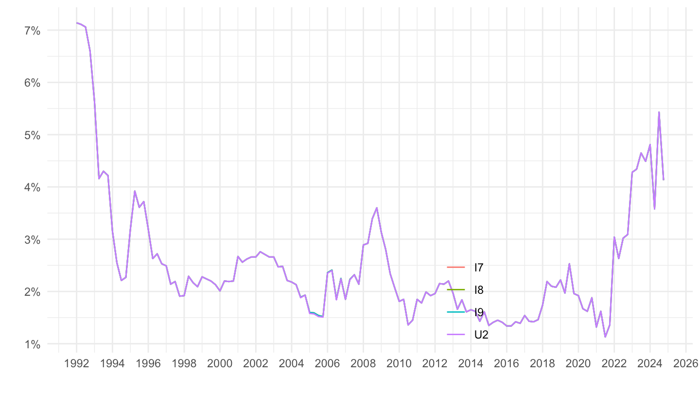
Annual
Code
STS %>%
  filter(STS_CONCEPT == "INWR") %>%
  filter(FREQ == "A") %>%
  year_to_date() %>%
  select(date, OBS_VALUE, REF_AREA) %>%
  ggplot() +  ylab("") + xlab("") + theme_minimal() +
  geom_line(aes(x = date, y = OBS_VALUE/100, color = REF_AREA)) +
  #scale_color_manual(values = viridis(4)[1:3]) +
  theme(legend.position = c(0.65, 0.15),
        legend.title = element_blank()) +
  scale_x_date(breaks = seq(1920, 2100, 2) %>% paste0("-01-01") %>% as.Date,
               labels = date_format("%Y")) +
  scale_y_continuous(breaks = 0.01*seq(0, 200, 1),
                     labels = percent_format(accuracy = 1))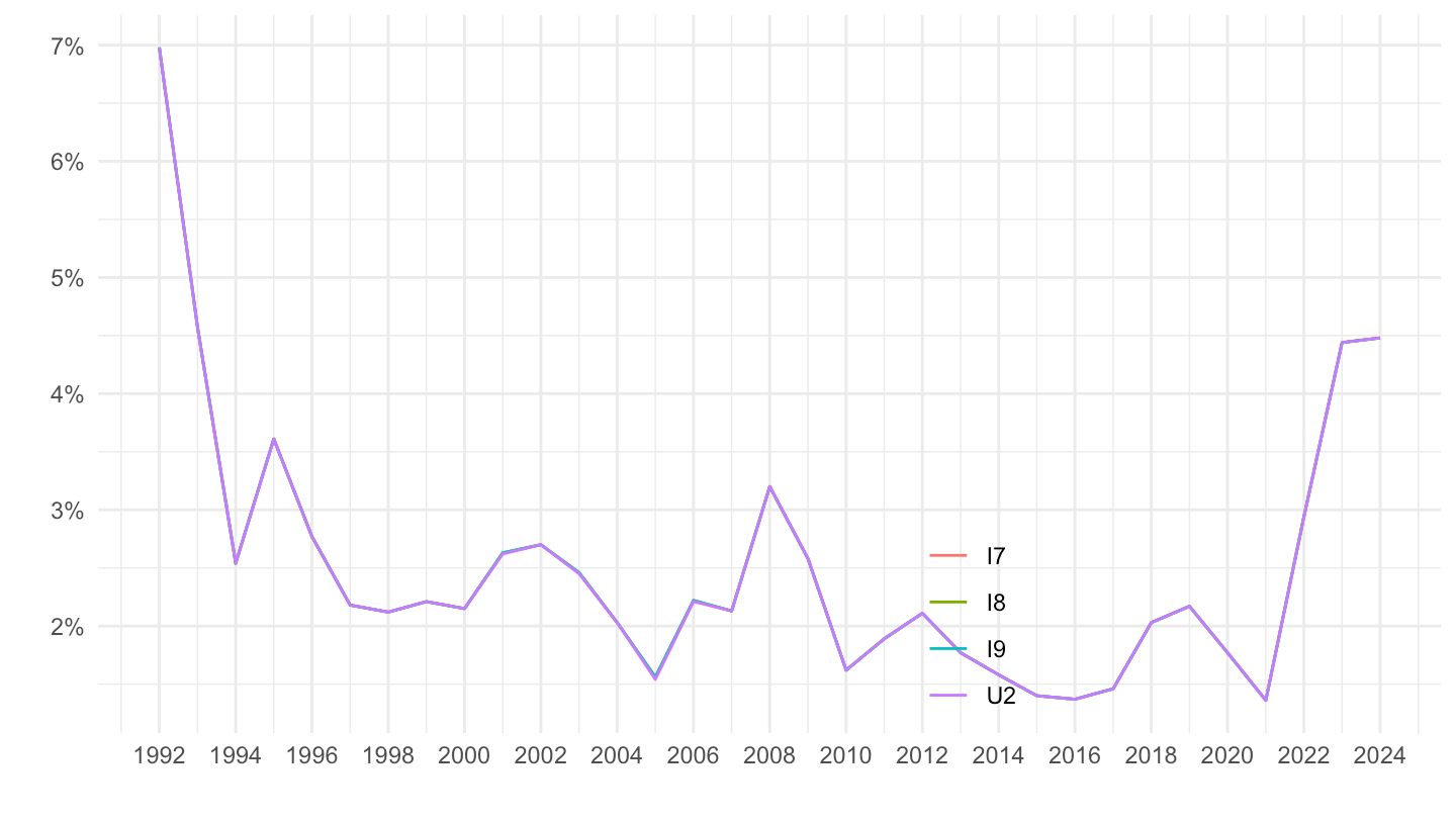
U2
All
Code
STS %>%
  filter(KEY %in% c("STS.Q.U2.N.INWR.000000.3.ANR")) %>%
  quarter_to_date() %>%
  select(date, OBS_VALUE, REF_AREA) %>%
  ggplot() +  ylab("") + xlab("") + theme_minimal() +
  geom_line(aes(x = date, y = OBS_VALUE/100)) +
  #scale_color_manual(values = viridis(4)[1:3]) +
  theme(legend.position = c(0.65, 0.15),
        legend.title = element_blank()) +
  scale_x_date(breaks = seq(1920, 2100, 2) %>% paste0("-01-01") %>% as.Date,
               labels = date_format("%Y")) +
  scale_y_continuous(breaks = 0.01*seq(0, 200, 1),
                     labels = percent_format(accuracy = 1))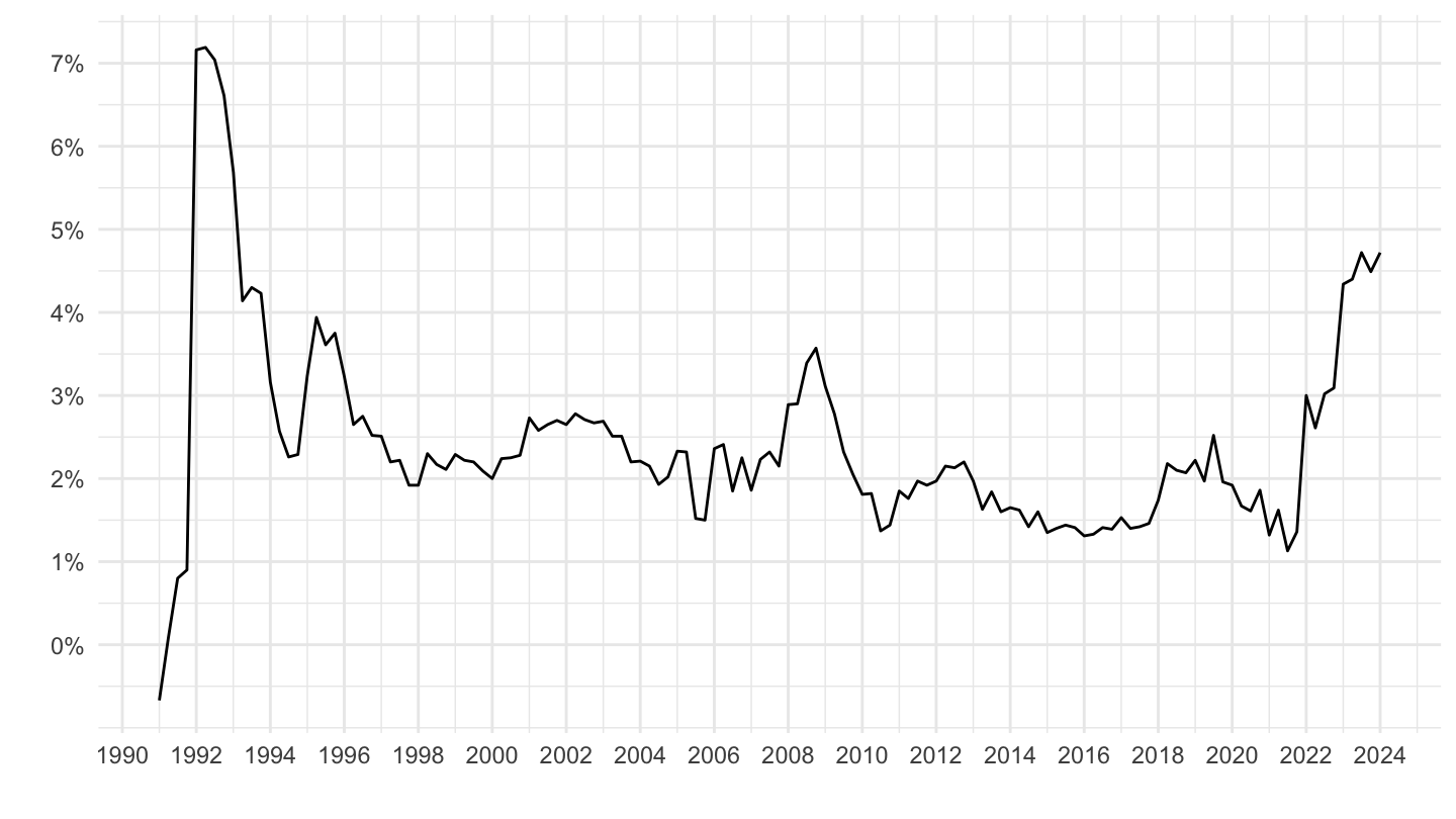
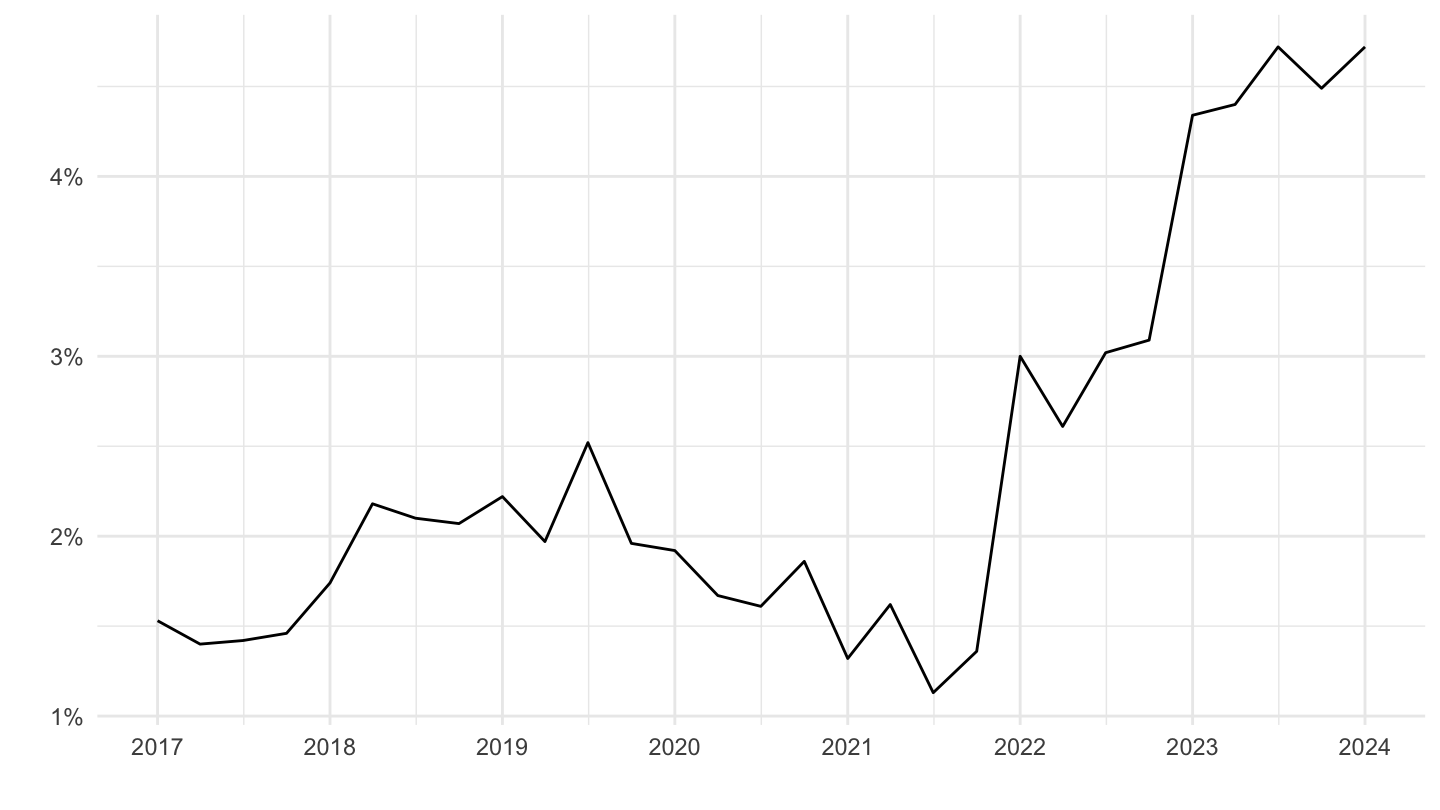
2017
Code
STS %>%
  filter(KEY %in% c("STS.Q.U2.N.INWR.000000.3.ANR")) %>%
  quarter_to_date() %>%
  filter(date >= as.Date("2017-01-01")) %>%
  select(date, OBS_VALUE, REF_AREA) %>%
  ggplot() +  ylab("") + xlab("") + theme_minimal() +
  geom_line(aes(x = date, y = OBS_VALUE/100)) +
  #scale_color_manual(values = viridis(4)[1:3]) +
  theme(legend.position = c(0.65, 0.15),
        legend.title = element_blank()) +
  scale_x_date(breaks = seq(1920, 2100, 1) %>% paste0("-01-01") %>% as.Date,
               labels = date_format("%Y")) +
  scale_y_continuous(breaks = 0.01*seq(0, 200, 1),
                     labels = percent_format(accuracy = 1))