14 Empirical Macroeconomics
Link to slides / Link to handouts
As we have seen in the previous lecture, macroeconomic theory alone often does not allow to conclude on the major issues that macroeconomists are trying to answer. For example, as we saw in problem set 8, models based on aggregate supply suggest that we should cut taxes on high income earners, while models based on aggregate demand suggest the opposite, based on different groups’ marginal propensities to consume.
Fortunately, macroeconomists are increasingly turning to empirical work to try and address these questions. During this lecture, I shall try to give you a very brief introduction to the rapidly expanding field of empirical macroeconomics.46 This field is rapidly evolving - most of the studies I will present to you are less than 10 years old. As I told you in the beginning of this class, macroeconomics is a rapidly changing field, where textbooks and views of the world are fast considered outdated. Thus, you should keep an open mind, and regularly update your knowledge of macroeconomics by reading The Economist Magazine for instance, which is usually good at covering the most up-to-date macroeconomics research.
Macroeconomists have three types of methodologies at their disposal, in order to try and answer empirical questions, which we will review in turn. We shall see that each one of these studies has advantages and drawbacks:
- Aggregate Studies
- Individual-Level Studies
- Cross-Sectional Studies
While presenting these studies, I will be focusing on what is probably the most important questions of all: the effect of fiscal policy on the macroeconomy.
14.1 Aggregate Government Spending Multipliers
John Maynard Keynes’ criticism of classical theory was born out of empirical observation of aggregate relationships. In “What has become of the Keynesian Revolution”, Joan Robinson reminds us of the political context in the UK at the beginning of the twentieth century, particularly following periods of high unemployment:
When Lloyd George proposed a campaign to reduce unemployment (which was then at the figure of one million or more) by expenditure on public works, he was answered by the famous “Trcasury View” that there is a certain amount of saving at any moment, available to finance investment, and if the government borrows a part, there will be so much the less for industry.
Joan Robinson reminds us that unfortunately (for mankind, and for people like me who would like to believe in the power of ideas), the nazis were a forerunner of J.M. Keynes, in that they had implemented Keynesian ideas way before these ideas had become mainstream:
Meanwhile the Nazis had been proving Lloyd George’s point with a vengeance. It was a joke in Germany that Hitler was planning to give employment in straightening the Crooked Lake, painting the Black Forest white and putting down linoleum in the Polish Corridor. The Treasury view was that his unsound policies would soon bring him down. But the little group of Keynesians was despondent and frustrated.
Probably the final empirical observation which led skeptics to definitively adopt Keynes’ ideas was the massive government spending which was undertaken in the U.S. during World War II, which put an end to the long-lasting depression which the U.S. never really came out of.
Since then, many studies have used government spending during wars in order to try to estimate the effect of government purchases on the macroeconomy. The reason for looking at wartime spending, is that wars are not usually supposed to be undertaken for reasons of macroeconomic stabilization. In contrast, most other discretionary government spending programs usually are meant to stabilize the economy. More generally, macroeconomists do not get to run “experiments”, with a clean treatment and control group like in medical research: periods in which government spending happens are usually different from periods when they don’t. This is why research progress in macroeconomics has been so slow and that disagreement is still so important (although it is narrowing).
A substantial amount of progress has been made since the 2007-2009 financial crisis, particularly following the various government spending programs which have been implemented throughout the world, and which provide a large number of new case studies. If you want to know more about government spending multipliers, and where macroeconomics research is right now on that issue, you may watch the video below of Valerie Ramey, one of the world’s most distinguished experts on the topic. Of course, this is not exam material, and you are not required to know anything more about aggregate studies concerning government spending multipliers.
Figure 14.1: National Bureau of Economic Research 2018 Conference: Ten Years after the Financial Crisis
14.2 Aggregate Tax Multipliers
Event studies. Donald Trump just passed a large tax cut through Congress (mostly in favor of high income earners). One approach to measuring the tax multiplier could simply be to look at what the effect on GDP growth will be of this tax cut, after it has been enacted. However, this approach (which is very much one that you will read about in the New York Times, or the Wall Street Journal, or on Donald Trump’s Twitter account!) is questionable, on at least two grounds:
The main issue is to know what the counterfactual would have been had Donald Trump not passed his tax cut. Many things happened in the meantime (this for example), so that the increase in GDP could not be due to the tax cut, but to other events which happened simultaneously. The tax cut which Donald Trump passed was not large enough for us to conclude without any ambiguity.
A second potential worry could be that Donald Trump may have decided on passing the tax cut for a reason; and that reason may have been that the economy was depressed to begin with. But if depressions tend to end without any government action, then the fact that the economy has rebounded could mistakenly be attributed to the tax cut, while it was more a return to normal. For this reason as well, it is very hard to conclude from one observation only.
Narrative approach. A more sophisticated version of the event study approach described above is called the narrative approach. It is exemplified by a paper of Romer and Romer (2010) in the American Economic Review.47 It is called “narrative” because the method consists in studying the motivation for each tax change, and focus on those tax changes that were not taken for the purpose of macroeconomic stabilization (“exogenous” tax changes). This addresses the second worry in the “event study” approach, that tax changes were not passed at random times. Second, studying many tax changes instead of just one, allows to address the first worry. With many tax cuts, other potential events happening simultaneously should average out to zero, and all the more that many of these events are being considered. Based on such an approach, the tax multiplier has been estimated to be quite large, on the order of 3. In other words, as shown in Figure 14.2, a 1% of GDP tax increase leads to a reduction in GDP of 2-3% over an horizon of 3 years - which symmetrically, implies that a 1% of GDP tax cut leads to an increase in GDP of 2-3% over a 3 year horizon. But let me quote Christina Romer, then head of the Council of Economic Advisors to the U.S. President, in her speech at the U.S. Monetary Policy Forum, on February 27, 2009:
To address the problem of omitted variables, David and I used narrative evidence to isolate tax changes uncorrelated with other factors affecting output. We read Congressional reports, Presidential speeches, the Economic Reports of the President, and other documents to identify relatively exogenous tax changes. We found that the estimated effect of these changes is very large. A tax cut of 1% of GDP raises GDP by between 2 and 3% over the next three years.
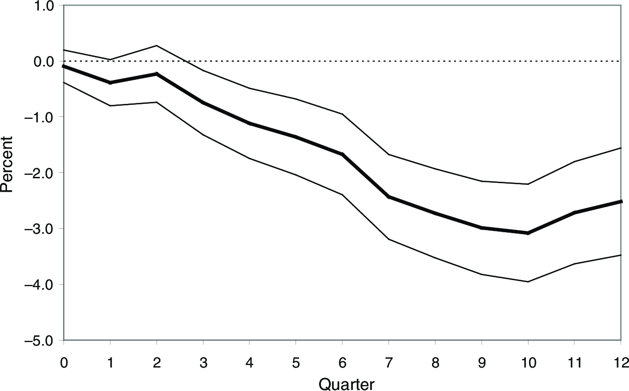
Figure 14.2: Impact on GDP of a 1% of GDP Aggregate Tax Increase. Source: Romer, Romer (2010).
The exact list of tax changes that Christina Romer and David Romer have considered is given on Figure 14.1, in a Table assembled by Owen Zidar, an assistant professor at Princeton University, whose study I shall talk about in Section 14.5. This table gives the motivation for these tax changes: most of the tax increases are taken to reduce the budget deficit, and most of the tax cuts are taken to improve the long-term prospect of the U.S. economy.
| Legislation | Year | Motiv | Exo? | Size |
|---|---|---|---|---|
| Revenue Act 1948 | 1948 | LR | Exo | -1.86 |
| Social Security Amendments 1947 | 1950 | Def | Exo | 0.26 |
| Internal Revenue Code 1954 | 1954 | LR | Exo | -0.37 |
| Social Security Amendments 1958 | 1960 | Def | Exo | 0.36 |
| Social Security Amendments 1961 | 1963 | Def | Exo | 0.86 |
| Revenue Act 1964 | 1964 | LR | Exo | -1.27 |
| Social Security Amendment 1967 | 1971 | Def | Exo | -0.02 |
| Revenue Act 1971 | 1972 | LR | Exo | -0.73 |
| Tax Reform Act 1976 | 1976 | LR | Exo | 0.13 |
| Tax Reduction & Simplif. Act 1977 | 1977 | LR | Endo | -0.38 |
| 1972 Changes to Social Security | 1978 | Def | Exo | 0.13 |
| Revenue Act 1978 | 1979 | LR | Exo | -0.39 |
| Social Security Amendment 1977 | 1981 | LR | Exo | 0.40 |
| Economic Recovery Tax Act 1981 | 1982 | LR | Exo | -1.33 |
| Economic Recovery Tax Act 1981 | 1983 | LR | Exo | -0.87 |
| Social Security Amendments 1983 | 1984 | Def | Exo | -0.41 |
| Social Security Amendments 1983 | 1985 | Def | Exo | 0.21 |
| Tax Reform Act 1986 | 1986 | LR | Exo | 0.60 |
| Tax Reform Act 1986 | 1987 | LR | Exo | -0.57 |
| Social Security Amendments 1983 | 1988 | Def | Exo | 0.37 |
| Social Security Amendments 1983 | 1990 | Def | Exo | 0.18 |
| Omnibus Budget Reconc. Act 1990 | 1991 | Def | Endo | 0.00 |
| Omnibus Budget Reconc. Act 1993 | 1993 | Def | Exo | 0.42 |
| Omnibus Budget Reconc. Act 1993 | 1994 | Def | Exo | 0.19 |
| Econ. Gth & Tax Relief Act 2001 | 2002 | LR | Exo | -0.77 |
| Jobs & Gth Tax Relief Reconc. Act 2003 | 2003 | LR | Exo | -1.13 |
| Jobs & Gth Tax Relief Reconc. Act 2003 | 2004 | LR | Endo | 0.00 |
| Jobs & Gth Tax Relief Reconc. Act 2003 | 2005 | LR | Exo | 0.54 |
Finally, Christina Romer and David Romer are also able to look at the effects of these tax increases on each individual component of aggregate demand. Panel A of figure 14.3 shows what the effects are of a 1% of GDP tax increase on consumption, investment and GDP: as we saw during this class, aggregate consumption declines, presumably a disposable income effect, investment declines because consumers demand less goods. Panel D of figure 14.3 shows that imports also decrease following a tax increase: some of the fall in demand implies also less demand for foreign goods. Something which we did not expect from lecture 11 is the behavior of exports, which slightly increase following a tax increase. This could be coming from the behavior of monetary policy, which may accommodate the negative fiscal shocks through lower interest rates (thus depreciating the dollar, and boosting exports). Finally, Panel B and C of figure 14.3 you cannot interpret, as we did not go into this level of detail: however you can note that the fall in consumption comes mostly from durables (like automobiles), which people stop purchasing first when they have a fall in their disposable income.
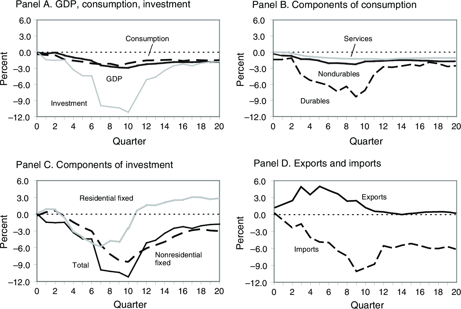
Figure 14.3: Impact on Individual Components of GDP of a 1% of GDP Aggregate Tax Increase. Source: Romer, Romer (2010).
Advantages and Drawbacks of Aggregate Studies. Aggregate studies such as Christina and David Romer’s have advantages and drawbacks:
On the positive side, aggregate studies are very transparent and simple. The results from these studies does not depend at all on economic theory, so that they may convince on either side of the political spectrum. They do not depend on people’s macroeconomic views (whether they believe in Say’s law, the Treasury View, and what not) and only “let the data speak.”
On the negative side, these studies are not always conclusive. They almost always are very noisy, in that we only have a handful episodes to look at. Finally, they do not allow to respond to more precise questions such as what is the impact of a tax cut on the bottom 90% versus that of a tax cut on the bottom 10%. The reason is that the episodes of tax cuts or tax increases are very few. Episodes where tax cuts are specifically on the rich or the poor are even more rare.
14.3 Individual-Level Labor Supply Elasticities
Individual-level studies allow to estimate key parameters that macroeconomists use in their models. Thus, this approach combines a mix of data and theory. The data allows to inform on parameters such as:
the Marginal Propensity to Consume \(c_1\), which is key for the demand-side view of tax cuts.
the “labor supply elasticity” \(1/\epsilon\), which is key for the supply-side view of tax cuts,
while on the other hand, theory is still useful in order to estimate tax and government multipliers as a function of these parameters, for example.
As we saw in problem set 8, many supply-side economists like Robert Barro take the view that tax cuts work not through disposable income effects (which he calls “heaping money to people”) but instead through reductions in their marginal tax rates, which incentivize them to work harder. Individual-level studies allow to very precisely estimate the importance of these effects, which Robert Barro believes to be sufficiently large to explain the entirety of output responses to tax cuts.
In the spirit of lecture 6 and problem set 8, let us consider again the utility function of a consumer-worker deciding how much to work, and whose utility of consuming \(c\) and working a number of hours \(l\) is given by: \[U(c, l)=c-B\frac{l^{1+\epsilon}}{1+\epsilon}.\] Further assume a linear tax rate on all income, and that this rate is given by \(\tau\) (in problem set 8, we had something more complex, with a bracket system, as well as a baseline level of consumption \(c_0\)), so that the budget constraint is: \[p \cdot c = (1-\tau)\cdot w \cdot l.\] The consumer-worker who chooses his number of hours does so in order to maximize the following utility: \[\max_l \quad (1-\tau)\frac{w}{p}l -B\frac{l^{1+\epsilon}}{1+\epsilon}\] leading to the following optimality condition: \[(1-\tau)\frac{w}{p}=B l^{\epsilon}.\] As in problem set 8, assume that the labor demand side is constituted of firms with a linear technology \(f(l) = A \cdot l\), which set the level of the real wage (again, see problem set 8 for detail) equal to their labor productivity, so that: \[\frac{w}{p}=A.\] As a consequence, the number of hours supply by the worker is simply given by: \[l=(1-\tau)^{1/\epsilon}\frac{A^{1/\epsilon}}{B^{1/\epsilon}}.\] Finally, income is given by the real wage times the number of hours: \[ \begin{aligned} y &= \frac{w}{p} \cdot l \\ &= A \cdot l \\ y &= (1-\tau)^{1/\epsilon}\frac{A^{1/\epsilon+1}}{B^{1/\epsilon}}. \end{aligned} \] Taking logs, we get income as a function of the tax rate \(\tau\), as well as \(A\) and \(B\): \[ \begin{aligned} \log(y) = \frac{1}{\epsilon}\log(1-\tau)+\left(\frac{1}{\epsilon}+1\right)\log A-\frac{1}{\epsilon}\log B. \end{aligned} \] As we saw in problem set 8, a change in taxes leads to a change in income such that: \[\frac{d \log(y)}{d \tau}=-\frac{1}{\epsilon (1-\tau)}.\] This formula allows to calculate \(1/\epsilon\) as a function of observed income responses to marginal tax changes. For example, imagine that we observe that when an individual’s marginal tax rate is decreased by 5% from \(\tau = 0.5 = 50\%\) to \(\tau+\Delta \tau = 0.45 = 45\%\), with \(\Delta \tau = -0.05 = -5\%\), this person has an increase in pre-tax income given by \(\Delta \log y = 0.05 = 5\%\). We would then be able to calculate a value for \(1/\epsilon\): \[\frac{1}{\epsilon}=(1-\tau)\frac{\Delta \log y}{-\Delta \tau}.\] In this example: \[\frac{1}{\epsilon} = \left(1-\frac{1}{2}\right) \cdot \frac{0.05}{0.05} = \frac{1}{2}.\] This corresponds to the situation of problem set 8. \(1/\epsilon\) is called the labor supply elasticity: the higher this number, the more income tends to respond a lot to changes in taxes (look at the formula above) - it is then said to be more “elastic” (“elastic” means “responds more” to changes in taxes). According to supply-side economists like Robert Barro, this elasticity is rather high. In other words, the number of hours responds a lot to taxes, which implies that output also increases a lot following reductions in taxes. Lower taxes motivate people to work more.
An emerging consensus is that this elasticity, which is precisely measured, is however not large enough to explain why tax cuts have such large effects. The maximum consensus estimate is 0.5, according to Raj Chetty and his coauthors (see here). Therefore, tax cuts must have aggregate demand effects, as Keynesian economics predicts.
14.4 Individual-Level Marginal Propensity to Consume (MPC)
The Marginal Propensity to Consume \(c_1\) is another such parameter, which is more relevant for the aggregate demand view of macroeconomics. But before we move to estimates of the MPC, I shall now come back to something which was henceforth hidden under the rug. There does not only exist one MPC but there are many such MPCs, depending on how persistent tax changes are.
As we saw in lecture 2, according to the neoclassical view of consumption, the MPC for a one year change in income, if the planning horizon is 30 years, is given by \(1/30\). The intuition is simple: people are supposed to be rational, look far into the future, and consume as a function of the present discounted value of their future income.
In contrast, if the tax shock is permanent, then people are expected to consume a much larger fraction of this additional income. In the case of low income people, they would even consume 100% of this income. In the case of higher income people, they would perhaps save a fraction of that, for example if they want to bequeath wealth to their children, or alternatively if they just do not know what to do with this additional money (see lecture 4 for a complete discussion of why rich people save).
I now describe the results from a recent study by Tullio Jappelli and Luigi Pistaferri called “Fiscal Policy and MPC Heterogeneity.” The marginal propensity to consume (MPC) which we look at here is the one which concerns a temporary income shock. This is relevant for the case of a temporary fiscal stimulus. The data in Figure 14.4 and Figure 14.5 show three things: that the MPC varies considerably across individuals, that it varies significantly as a function of their income, and more importantly, that it is much larger on average than the theory of rational consumers would lead us to believe (it is closer to 25% than to 3%).
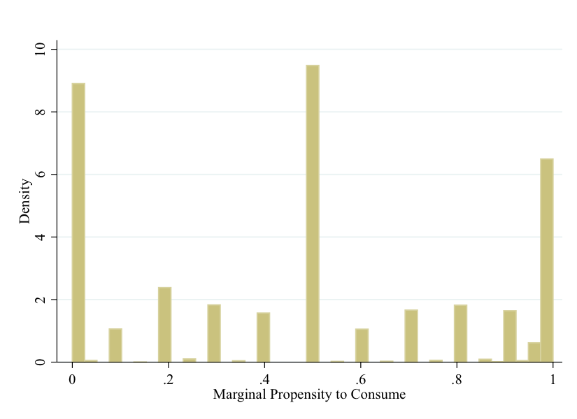
Figure 14.4: Self-Reported MPC from Transitory Income Shock. Source: Jappelli, Pistaferri (2014).
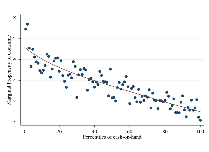
Figure 14.5: Average MPC By Cash-On-Hand Percentiles. Source: Jappelli, Pistaferri (2014).
14.5 Cross-Sectional Studies
Finally, of all methods, cross-sectional studies are probably the most promising, and are increasingly being used to arrive at credible estimate of fiscal multipliers.
In a forthcoming Journal of Political Economy paper, Owen Zidar, an assistant professor at Princeton University, has estimated the effect of tax cuts, as Romer and Romer (2010), using state-level variation as an identification strategy. Variation in the income distribution across U.S. states leads to heterogeneous regional impacts of federal income tax changes. For instance, Connecticut, whose share of top-income taxpayers is nearly twice that of the typical state, faced relatively larger shocks to high-income earners after the Omnibus Budget Reconciliation Act of 1993, which raised top- income tax rates.
Figure 14.6 shows that different tax reforms lead to very different redistributive effects on various groups in the population. In 1982, the tax cut mostly benefited higher income households. In 1993 in contrast, Bill Clinton’s tax bill led to a substantial increase in high earners’ taxes. The schedule that he chose is shown on Figure 14.7.
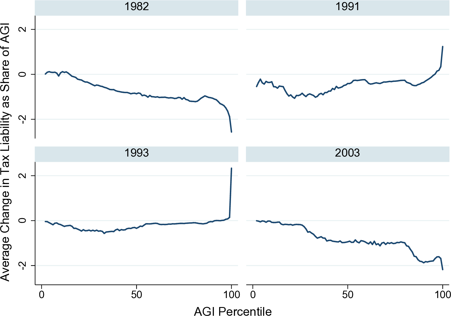
Figure 14.6: Various Types of U.S. Tax Reforms. Source: Zidar (2018).
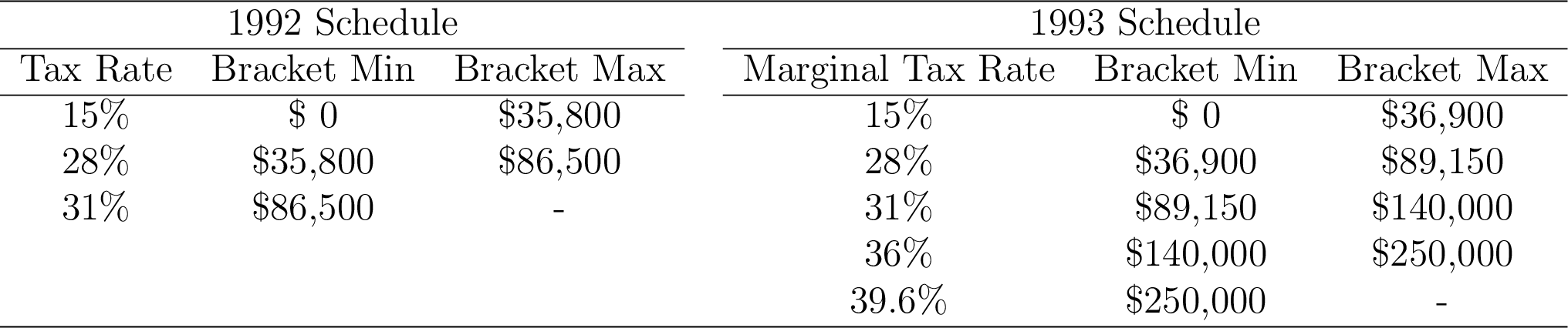
Figure 14.7: An Example of Tax Increase on High Income Earners: 1992 and 1993 Income Tax Schedules. Source: Zidar (2018).
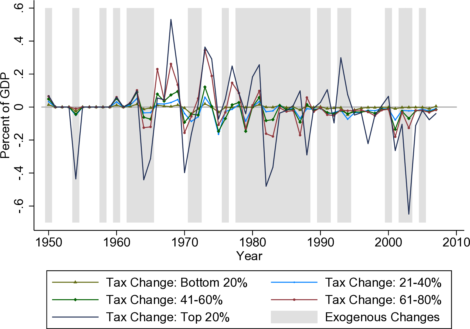
Figure 14.8: Federal Income and Payroll Tax Changes by AGI Quintile. Source: Zidar (2018).
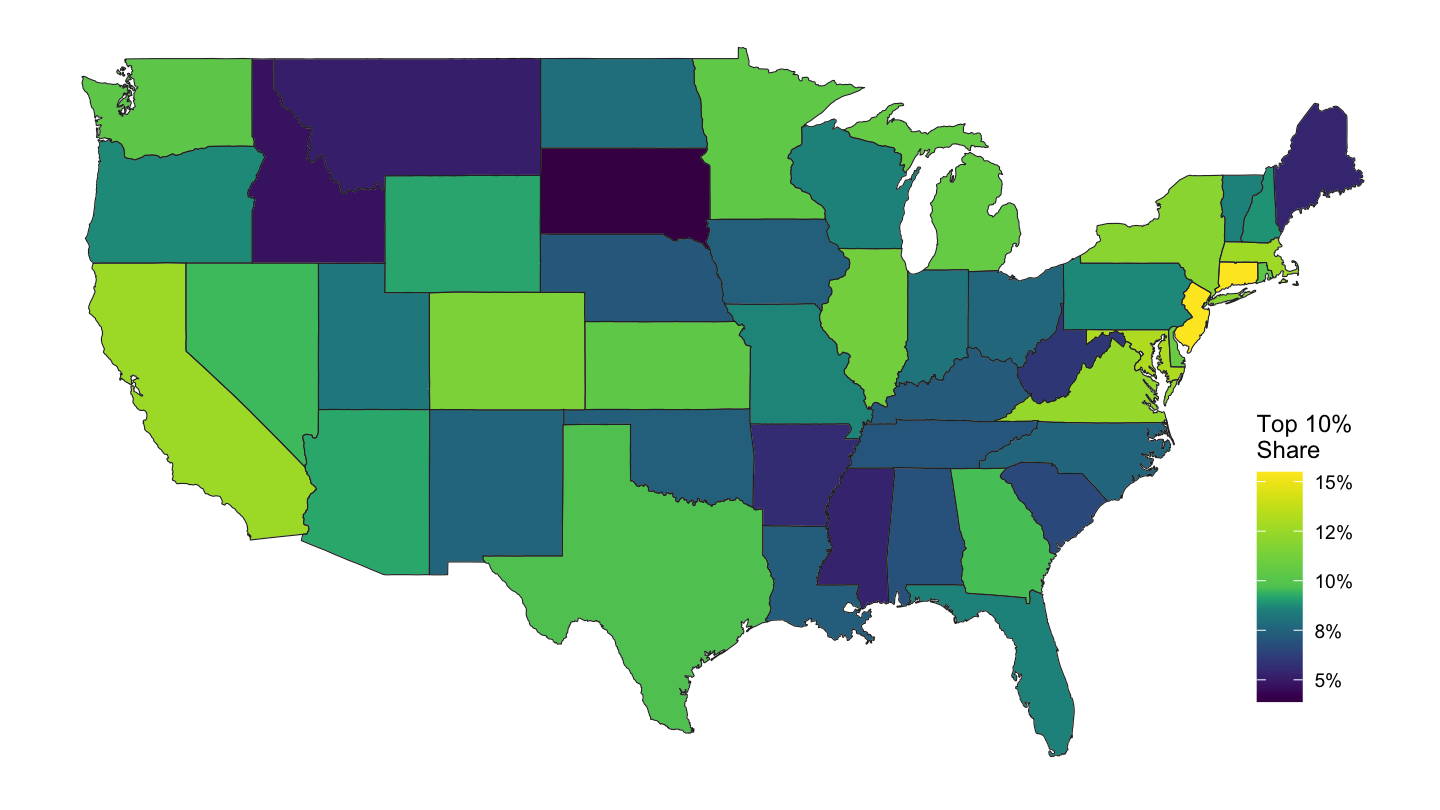
Figure 14.9: Share of High-Income Taxpayers. Source: Zidar (2018).
The estimated effects of such tax reforms on employment to population ratios, employment, and real GDP are shown on Figure 14.10, Figure 14.11 and 14.12.
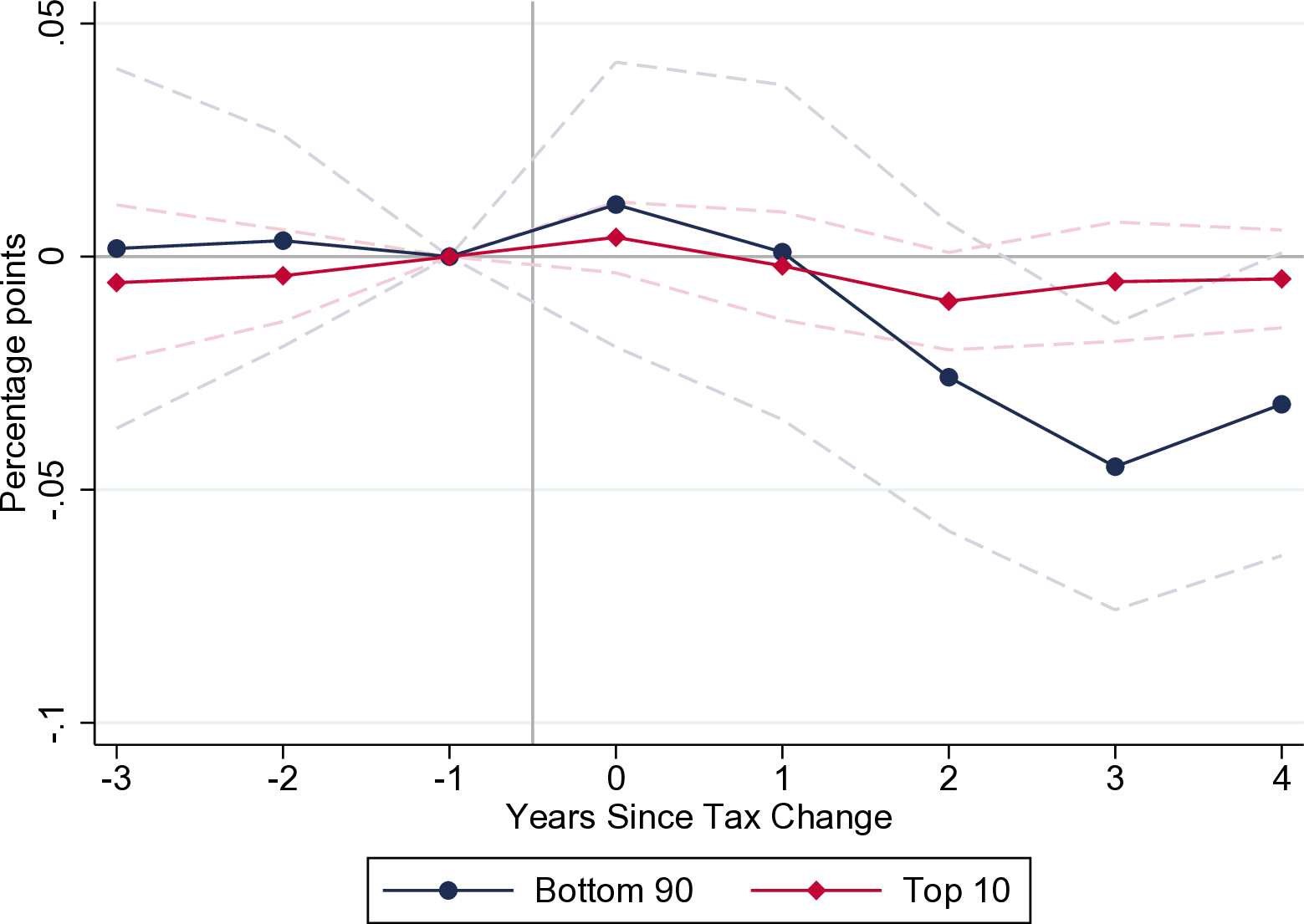
Figure 14.10: Employment to Population Ratio. Source: Zidar (2018).
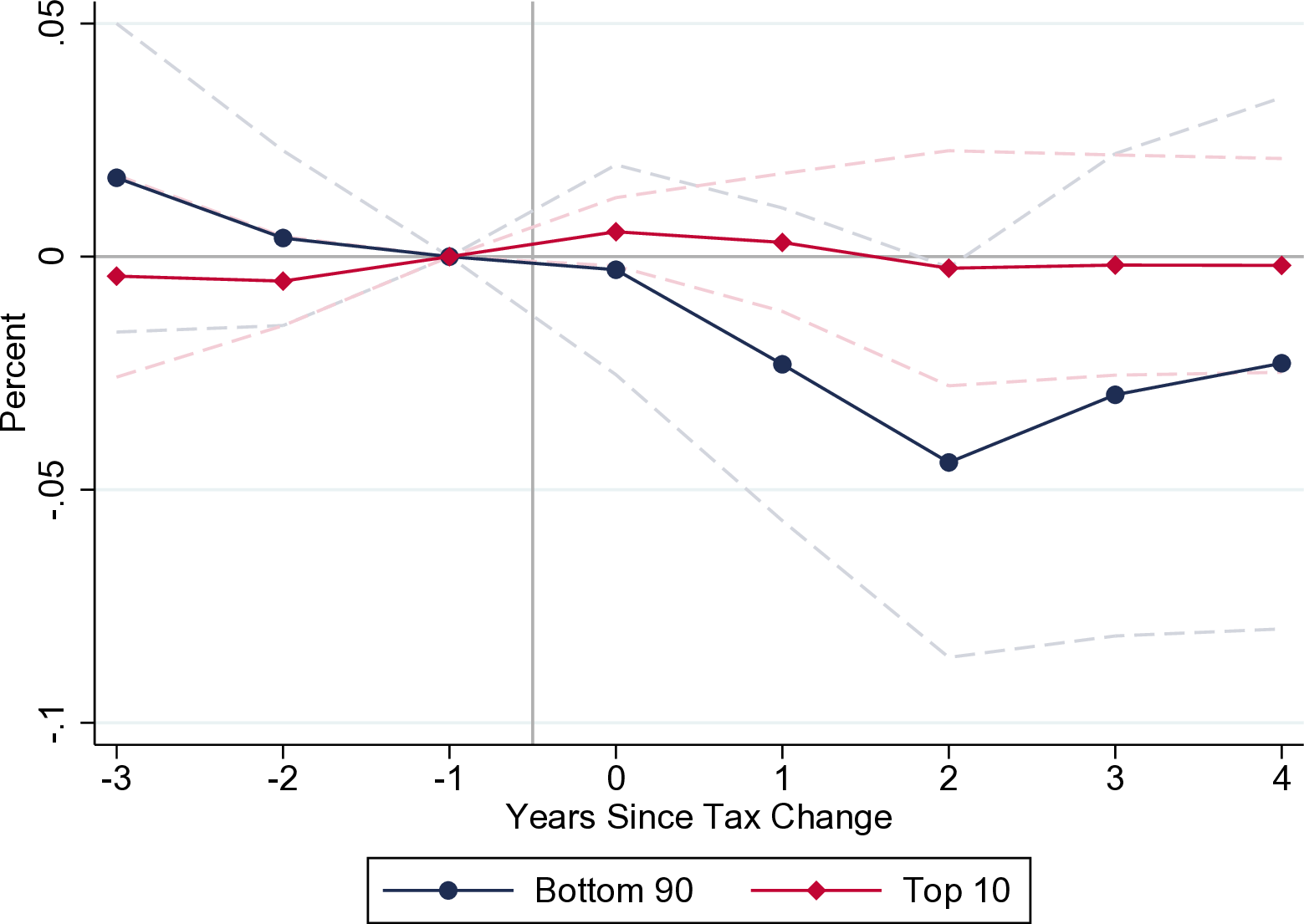
Figure 14.11: Employment. Source: Zidar (2018).
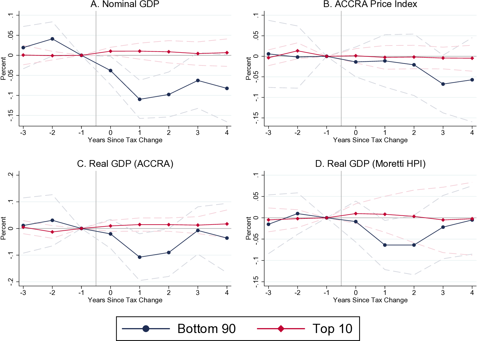
Figure 14.12: Nominal GDP, Real GDP, Price Indexes. Source: Zidar (2018).
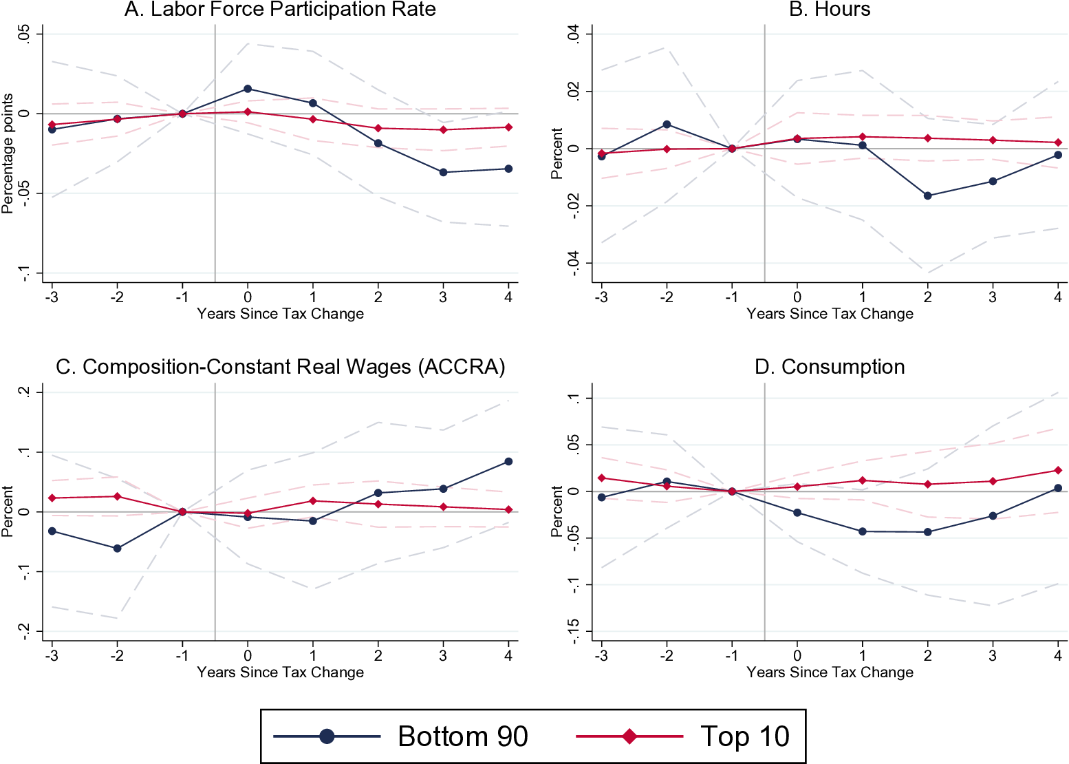
Figure 14.13: Participation, Hours, Real Wages, Consumption. Source: Zidar (2018).
Additional Readings
Paul Krugman, Multipliers and Reality, New York Times Blog Post, June 3, 2015.
I wish I was able to do more than just one lecture on that. Unfortunately, I am supposed to teach a class entitled “Macroeconomic Theory”, so I had to focus mostly on different macroeconomic theories, rather than on the supporting evidence.↩
Christina D. Romer and David H. Romer, “The Macroeconomic Effects of Tax Changes: Estimates Based on a New Measure of Fiscal Shocks,” American Economic Review 100, no. 3 (June 2010): 763–801. https://doi.org/10.1257/aer.100.3.763↩