December 4, 2019
Aggregate Studies
The Problem with Empirical Macro 1/3


The Problem with Empirical Macro 2/3
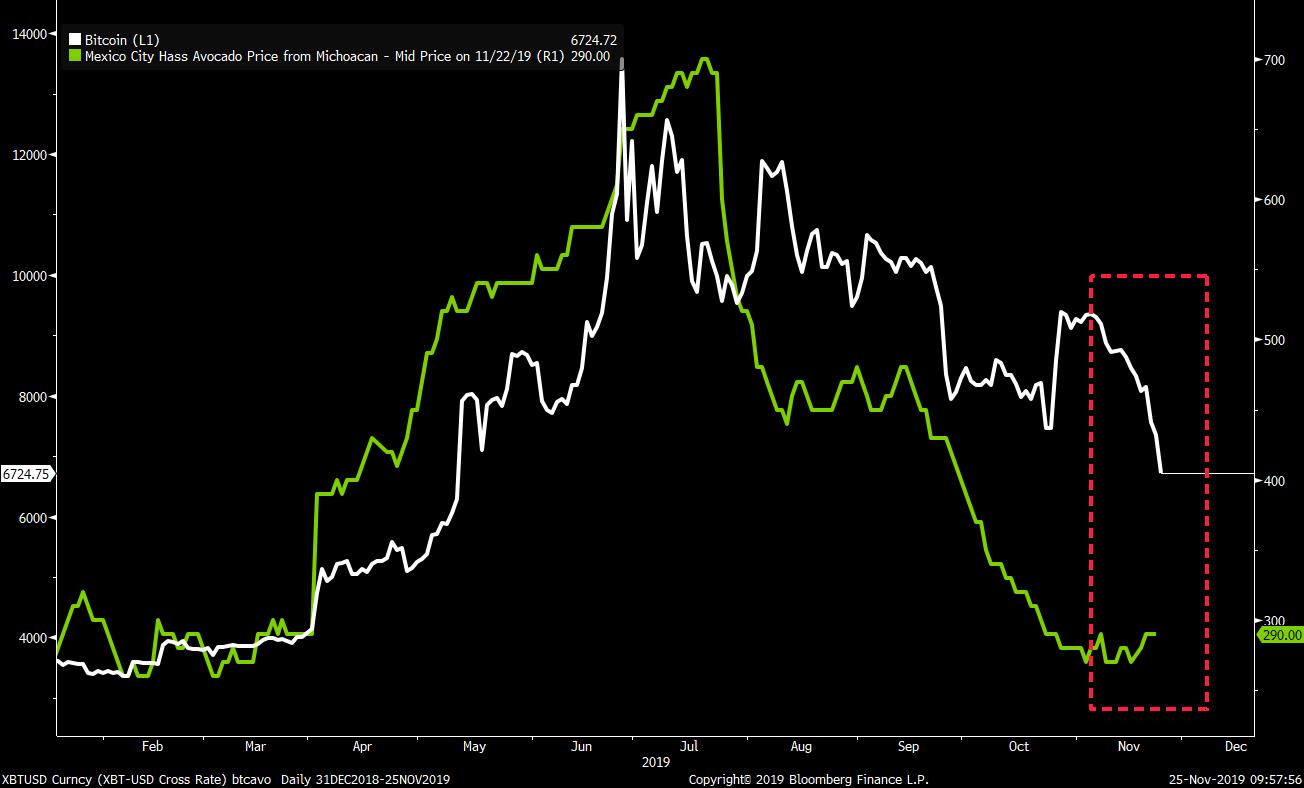
The Problem with Empirical Macro 3/3
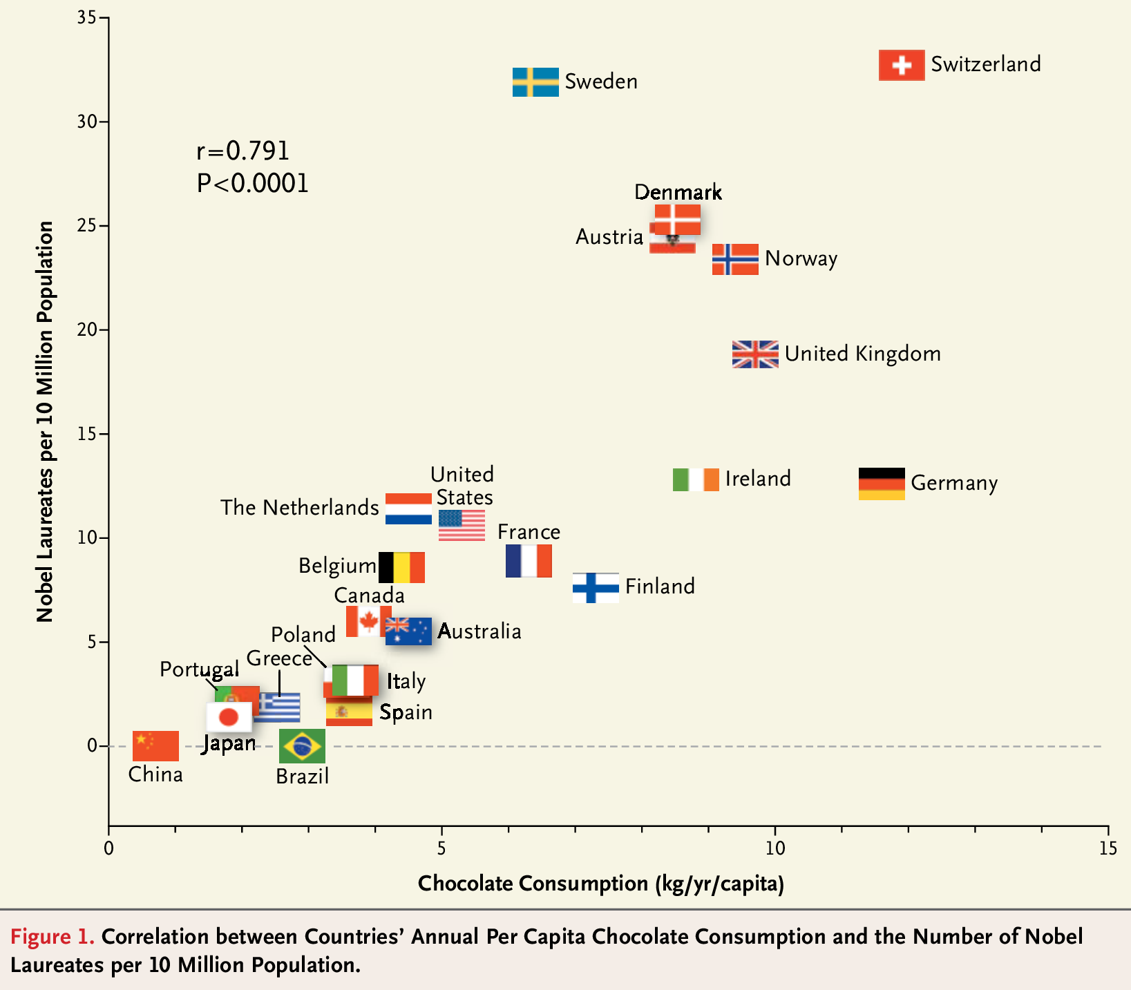
Messerli (2012): Nobel Laureates and Chocolate Consumption.
The Problem with Empirical Macro
Why don’t we just look at what happens to GDP following a tax cut?
Many things happen in any one year:
– September 15, 2013: Britney Spears happens to release her new song, which promotes work ethic.
– However, other things have happened between 2013 and 2018 (including a massive tax cut plan)Policies are changed for a reason:
– Years where taxes are changed are different from taxes where taxes are not changed.
– This is not like a Randomized Control Trial (RCT) in medicine: macroeconomic policies are not changed randomly.
– For example: \(\Delta G>0\) often happens during recessions. Low subsequent GDP growth: low multipliers or because GDP growth was low to start with.
Answers
What are the potential answers?
Add up many tax changes:
Some tax changes are accompanied by a new release of Britney Spears, but on average they are not.
Allows to control for other types of more serious events, too. (wars, etc.)
State their motivations:
Taxes raised to reduce the deficit, or increase long-run incentives are “exogenous.”
We do not want to look at tax changes which are made for managing the business cycle, in particular.
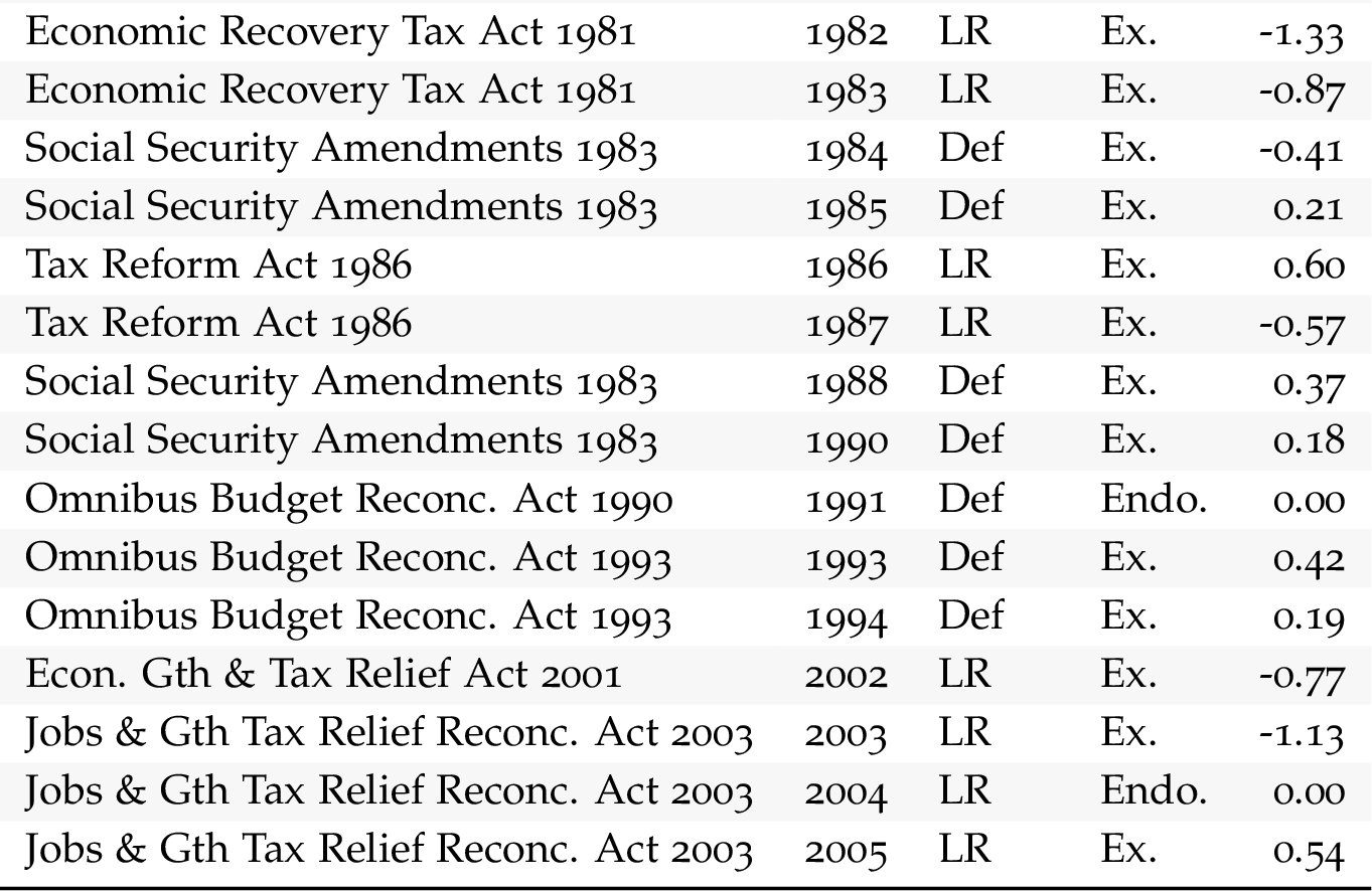
List of Tax Changes 1/2
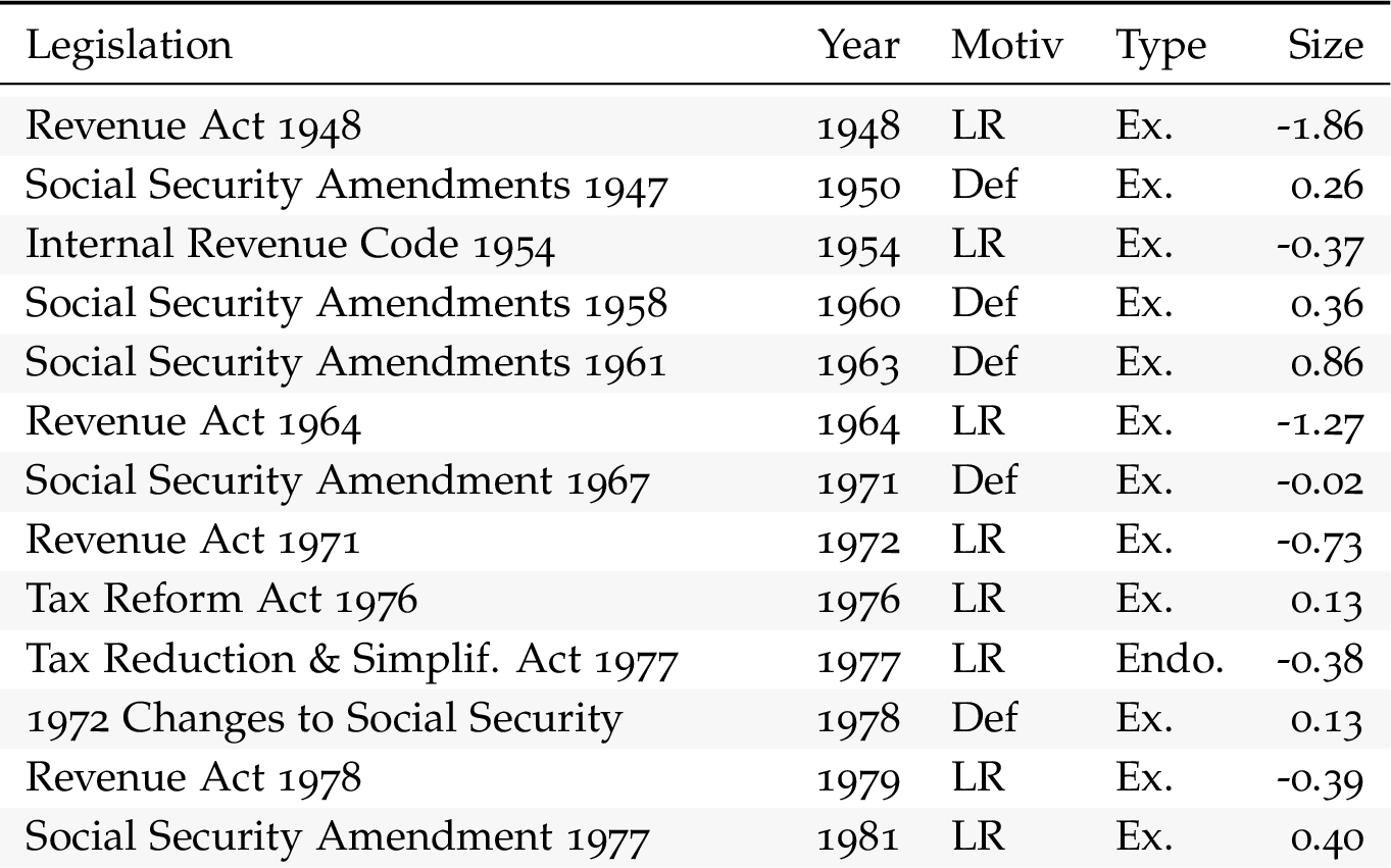
List of Tax Changes 2/2
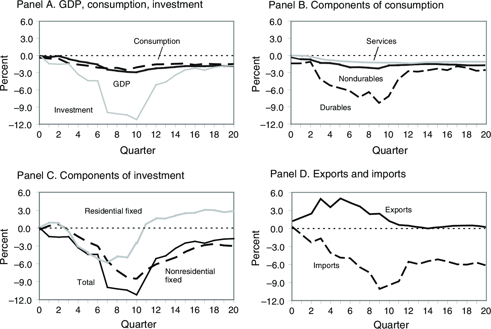
Tax Increase, 1% of GDP (Romer and Romer (2010))
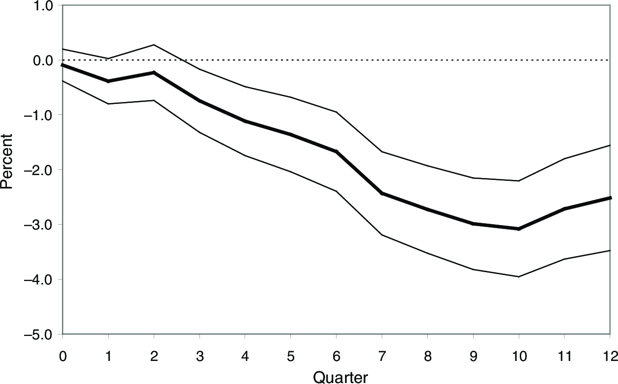
Romer and Romer (2010)
Advantages and Disadvantages
Issues with these studies:
– Noisy results: multiplier is between 2 and 4.
– One cannot further decompose: e.g. Top 10% VS Bottom 90%. We would get something even noisier.
– Always worry that tax changes are endogenous. (at the aggregate level, taxes are changed for a reason)
Advantages:
– It is exactly the object of interest (national level multiplier).
– Allows to tell apart different models.
Individual-Level Studies
Advantages and Disadvantages
Using individual-level data like survey, fiscal, administrative, or account-level data to measure \(\epsilon\), or \(c_{1}\). Advantages:
– Many more individuals: less noisy results (more observations).
– More credible “identification”: comparing two people at the same time period.
Disadvantages:
– Keynesian, aggregate demand effects cannot be estimated.
– e.g. if I decrease someone’s tax rate, then it might lead someone else to work more, not just the person who benefited from the fall in tax rates. (though the aggregate demand effect).
– Thus, there is no clean “control” group if there are aggregate demand effects.
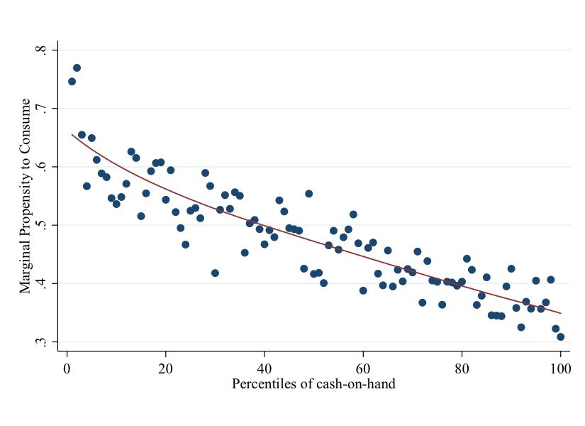
MPC (Jappelli and Pistaferri (2014))
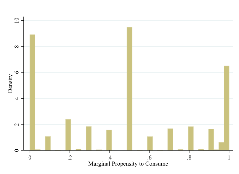
MPC (Jappelli and Pistaferri (2014))
Cross-sectional Studies
Advantages and Disadvantages
Identification across zipcodes, counties, or states. Advantages:
– More observations.
– Measure Keynesian, aggregate demand, general equilibrium effects.
– Less endogenous changes than at the national level: aggregate taxes are not changed in the U.S. to target California’s GDP specifically.
Disadvantages:
– Openness \(m_{1}\) of a state is larger, so multiplier is lower.
– But we are interested in national level multipliers, not state level multipliers.
– We thus need economic theory in order to infer national multipliers from state multipliers.
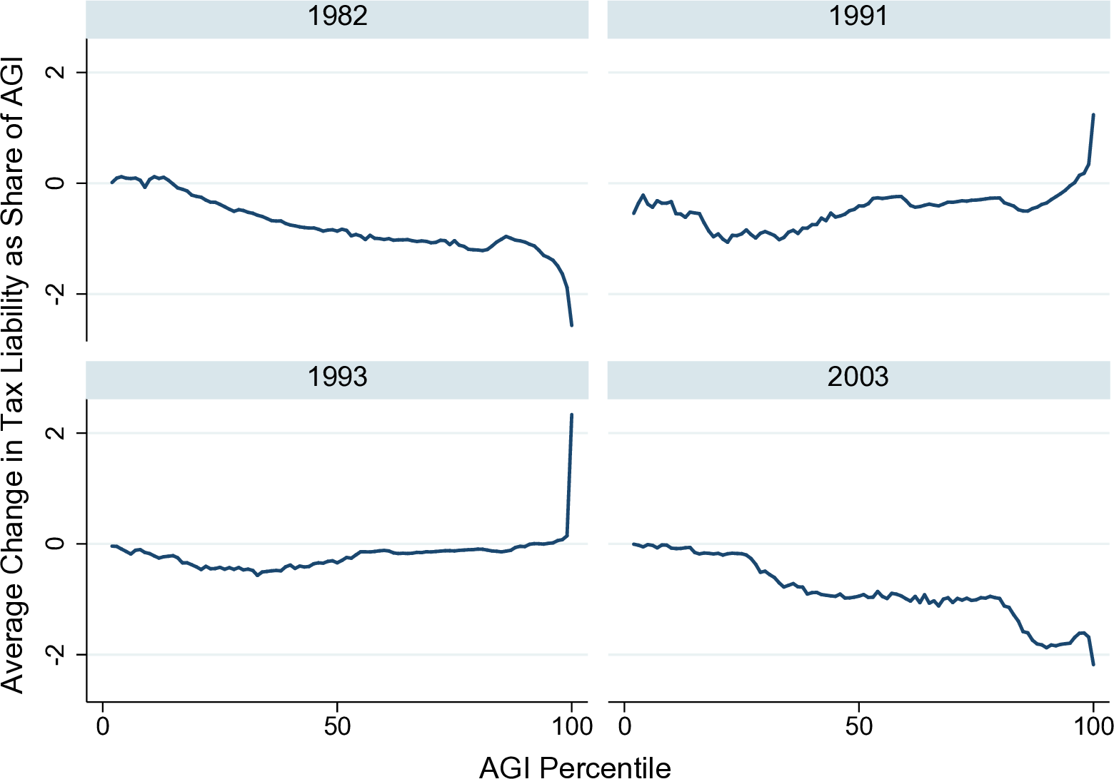
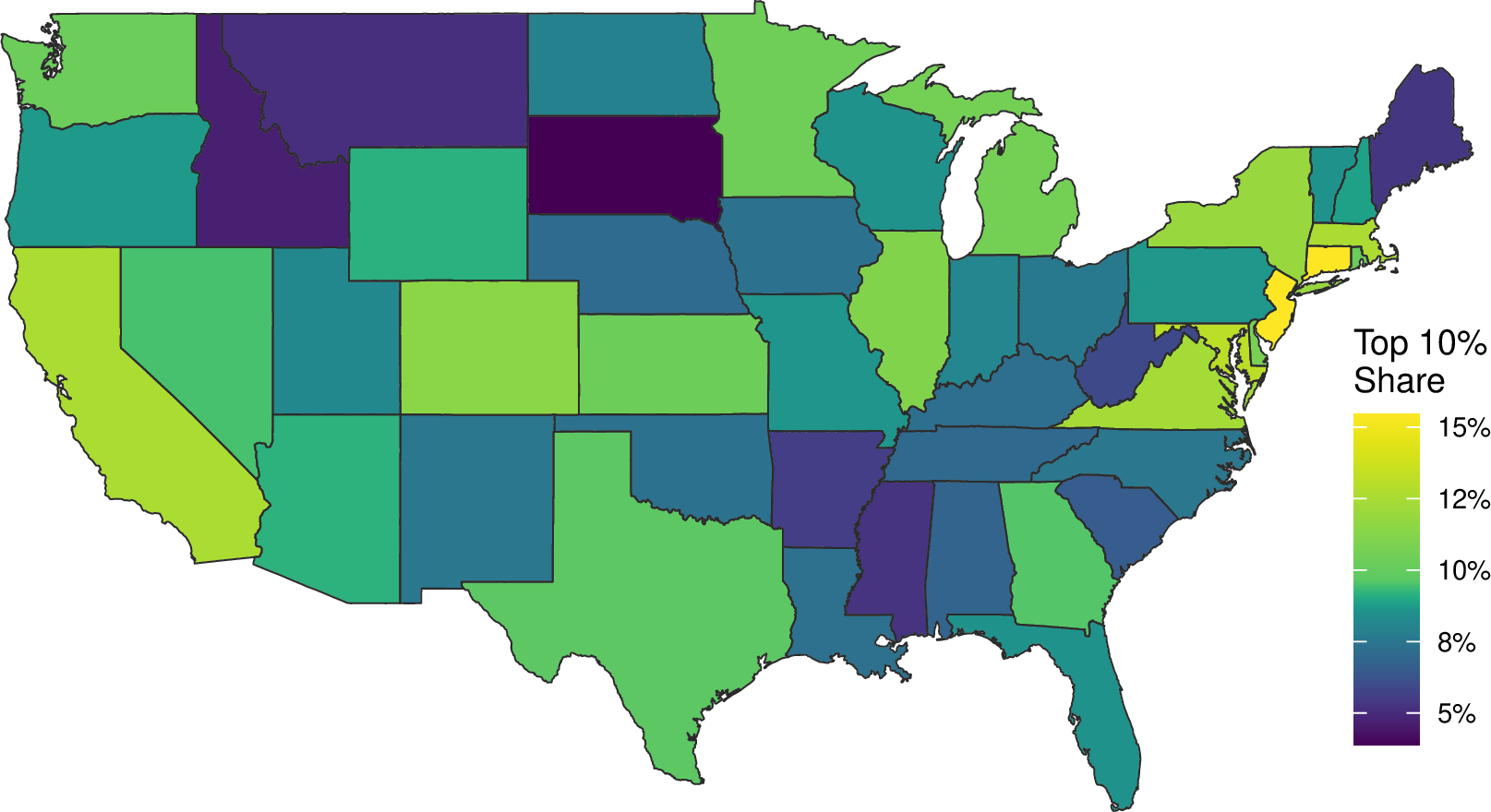
Zidar (2019): “Tax Cuts for Whom?”
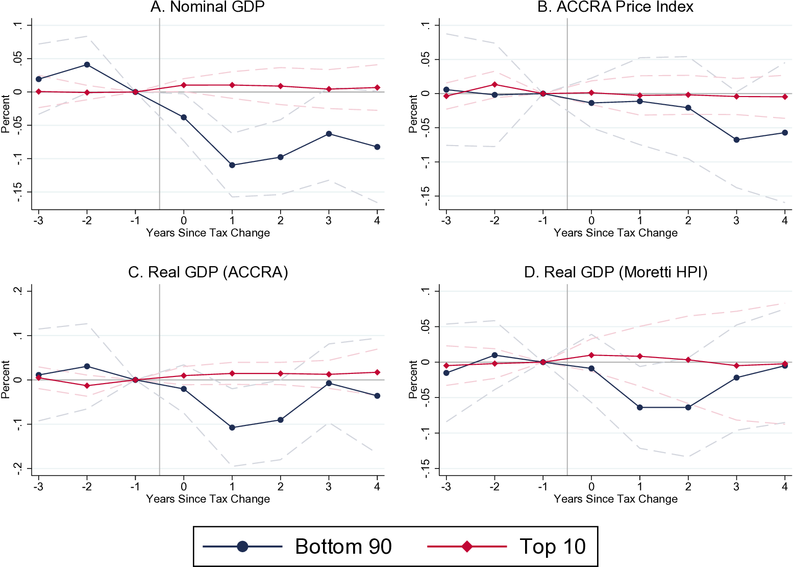
Using state-level variation in income distributions, Zidar (2019) in a Journal of Political Economy paper named “Tax Cuts For Whom? Heterogeneous Effects of Income Tax Changes on Growth and Employment” estimates the following effects on GDP:
– Multiplier effect of a tax cut to the bottom 90% is roughly 7.
– Multiplier effect of a tax cut to the top 10% is roughly 0.
– A tax cut going half to both groups has a multiplier of about 3.5 (Romer, Romer (2010) result).
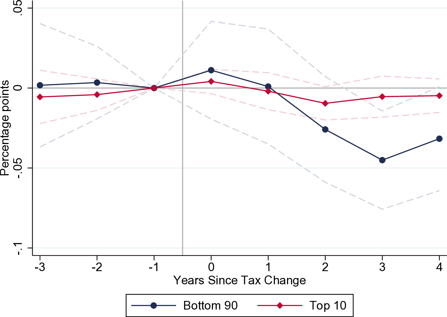
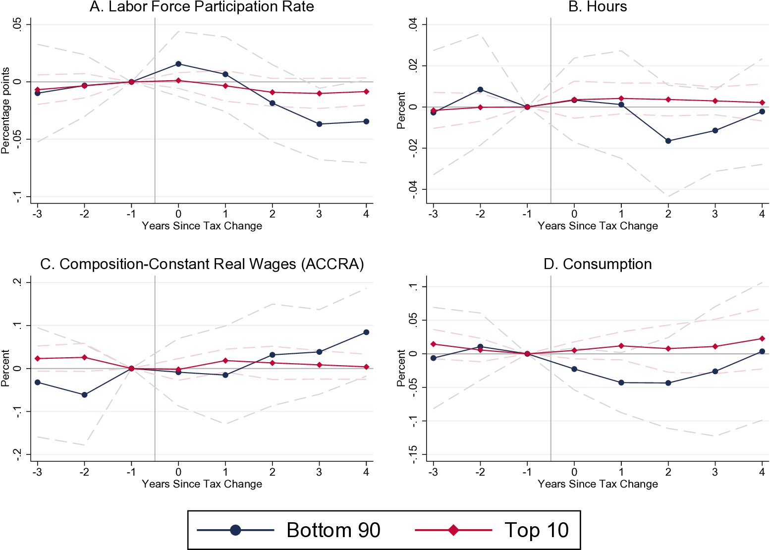
Zidar (2019): “Tax Cuts for Whom?”
Results seem to confirm our results from Lecture 9: tax cuts on bottom 90% work better than on top 10%.
Effects on employment are similar:
– 1% of state GDP tax cut for the bottom 90% results in 3.4% employment growth over a 2-year period.
– 1% of state GDP tax cut for the top 10% is 0.2% and statistically insignificant.
Zidar (2019)
Zidar (2019)
Zidar (2019)
Zidar (2019)
Zidar (2019)
Conclusion
Additional Watching (Not Required)
Taking Stock
Value of the Keynesian multiplier is still subject to very intense debates.
Tax-based multipliers > government spending multipliers (because tax changes are more persistent?)
Tax-based multipliers could be as high as 3.
Evidence that tax changes have long-term effect. There is a paradox of thrift.
My view: the evidence is more supportive of the Keynesian model, than of the neoclassical model.
Disclaimer: not everyone agrees with that view, and you are perfectly free to disagree too!
Bibliography
Jappelli, Tullio, and Luigi Pistaferri. 2014. “Fiscal Policy and MPC Heterogeneity.” American Economic Journal: Macroeconomics 6 (4): 107–36. https://doi.org/10.1257/mac.6.4.107.
Romer, Christina D., and David H. Romer. 2010. “The Macroeconomic Effects of Tax Changes: Estimates Based on a New Measure of Fiscal Shocks.” American Economic Review 100 (3): 763–801. https://doi.org/10.1257/aer.100.3.763.
Zidar, Owen. 2019. “Tax Cuts for Whom? Heterogeneous Effects of Income Tax Changes on Growth and Employment.” Journal of Political Economy 127 (3): 1437–72. https://doi.org/10.1086/701424.