12 Monetary Policy
Link to slides / Link to handouts
The late Rudi Dornbusch, an economist at the Massachusetts Institute of Technology, once remarked: “None of the postwar expansions died of old age, they were all murdered by the Fed.” It is indeed a fact that, as we shall notice during this lecture, every recession since 1945, was preceded by central banks raising interest rates. (usually, the reason which was given was a rise in inflation) how and why do central banks raise interest rates? Are they really that powerful, and in particular are they indeed responsible for recessions? We take up this issue in this chapter.
In the United States, the Federal Reserve System, a quasi-independant part of the government (at least up to now !), is responsible for setting monetary policy. The U.S. Federal Reserve chooses the level of the short term interest rate, either the federal funds rate or the discount rate. Figure 12.1 plots the Federal Funds rate for the 1953-2019 period, and the Discount Rate for the 1914-1953 period.
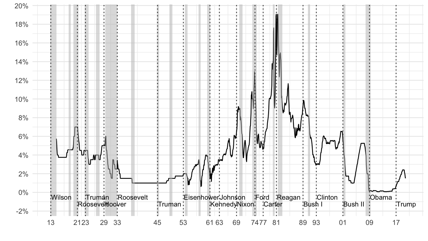
Figure 12.1: U.S. Federal Funds Rate, or Discount Rate (1914-2019).
An important component of monetary policy is a choice of the exchange rate regime. For example, the U.S. was on the Gold standard for most of its history, as shown on Figure 12.3: throughout most of the period, the price of Gold was fixed in dollars. The dollar was famously devalued against gold by F.D. Roosevelt in Spring 1933, as can be shown on Figure 12.3 below.
On August 15, 1971, the U.S. decided to end the convertibility of the dollar into Gold (the “Nixon shock”), as shown on Figure 12.4.
Figure 12.2: Nixon Address, August 15, 1971.
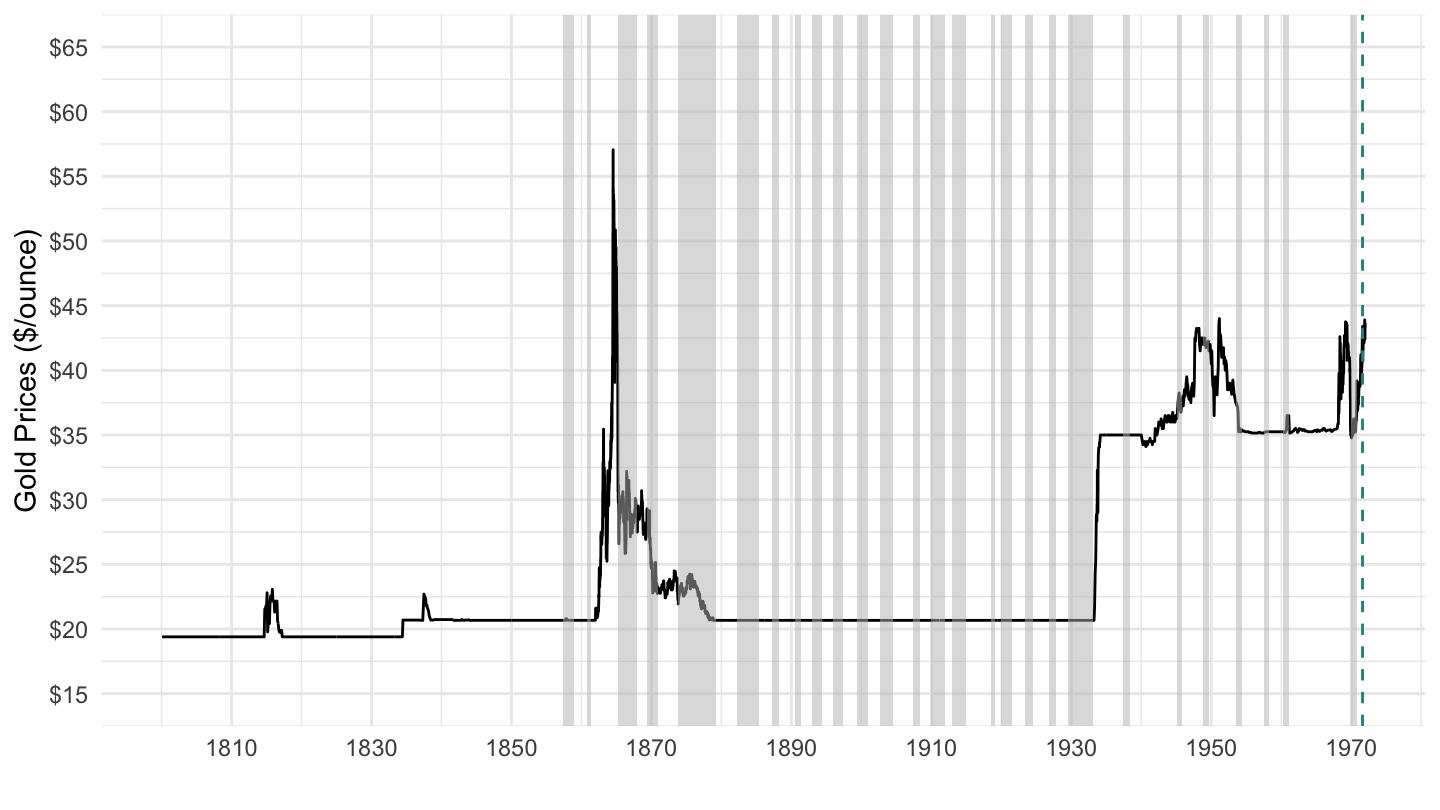
Figure 12.3: Gold Prices ($/Ounce) 1800-1972
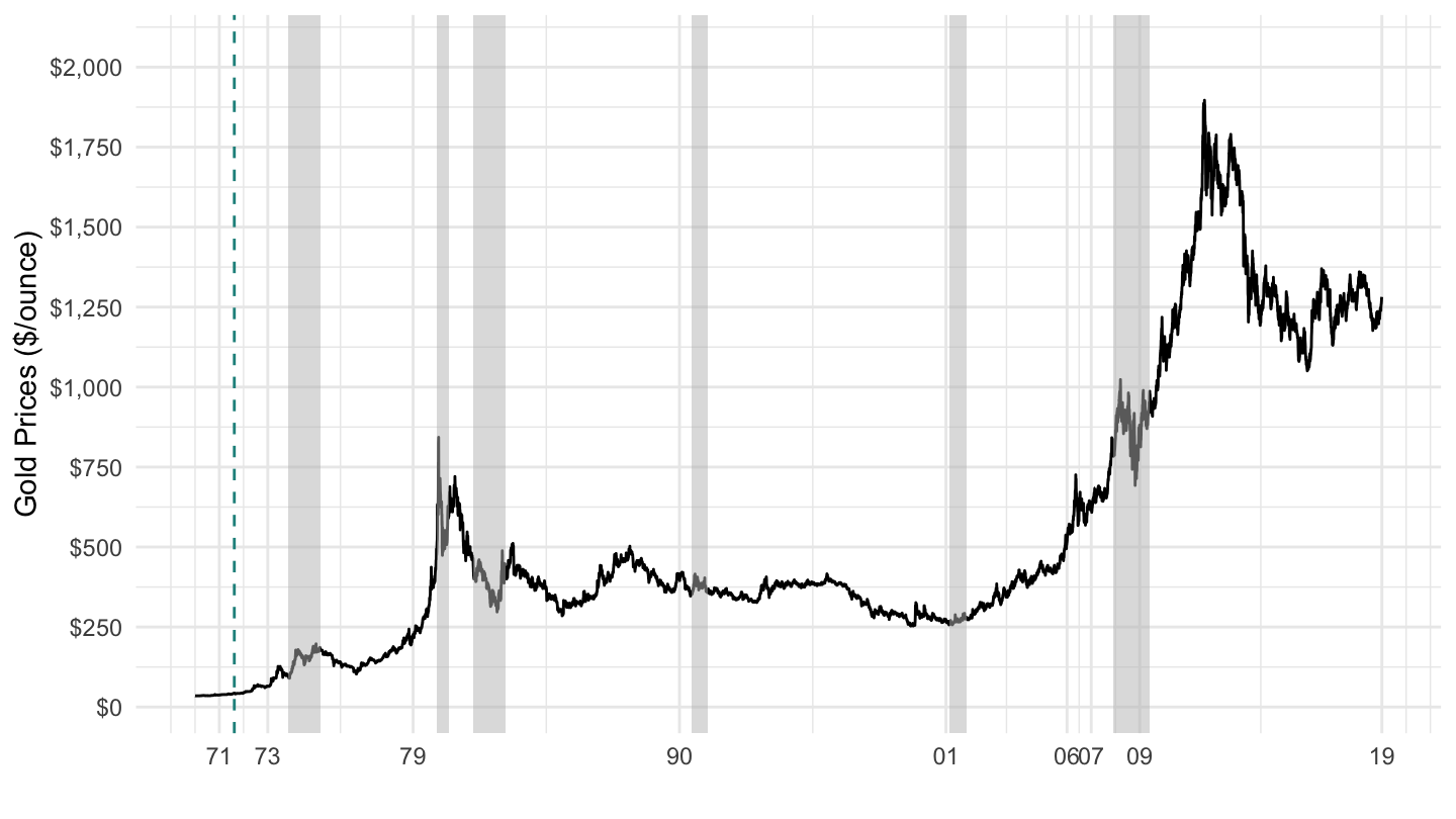
Figure 12.4: Gold Prices ($/Ounce) 1970-2019.
The switch from the Gold Standard to inflation targeting is shown on Figure 12.5 and Figure 12.6, with the Nixon shock on August 15, 1971.
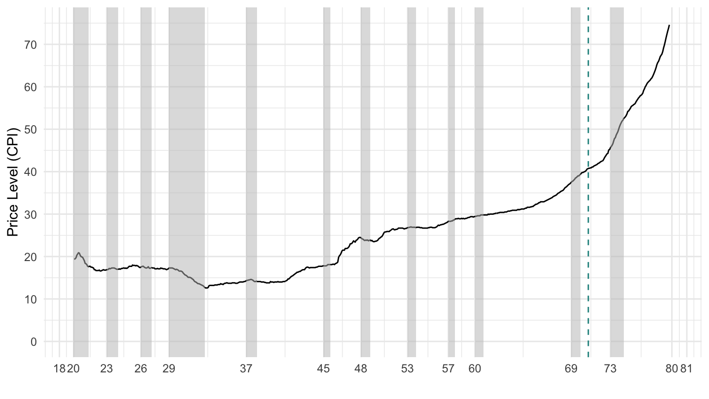
Figure 12.5: U.S. Price Level 1920-1980.
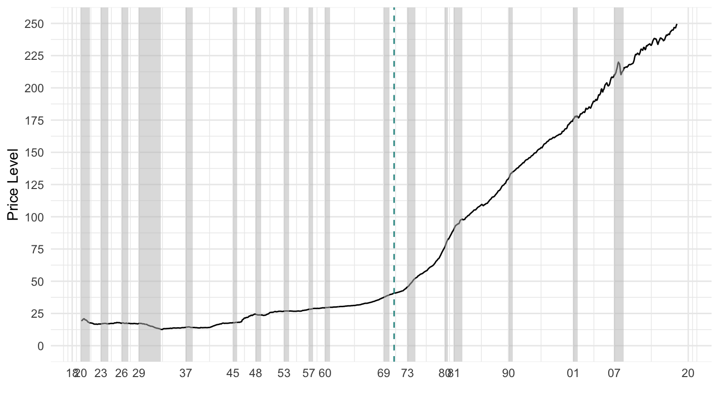
Figure 12.6: U.S. Price Level 1920-2019.
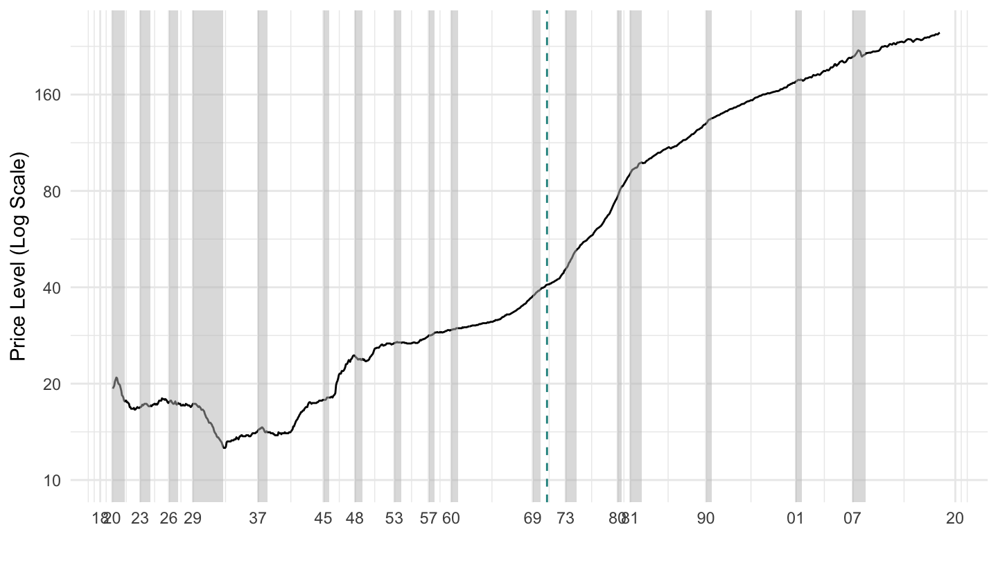
Figure 12.7: U.S. Price Level 1920-2019 (Log Scale).
Since then, the short term interest rate set by the Federal Reserve may impact the economy through two main channels:
the exchange rate channel. By affecting the level of interest rates, the central bank is able to affect nominal exchange rates, and, at least in the short-run, real exchange rates (because prices are sticky). Lower interest rates lead to a lower nominal exchange rate, and therefore, in the short run, to a lower real exchange rate. Devaluations make exports more competitive, and imports more expensive: they may therefore increase exports and reduce imports.
the credit channel. In the U.S. and in the U.K., many homeowners borrow at a rate close to the rate set by the Federal Reserve. With adjustable rate mortgages, the payments of these borrowers automatically follow short term interest rates. When interest rates go up, these payments increase. When interest rates go down, these payments decrease. Moreover, most households may refinance their loans when interest rate go down; this also allows them to reduce their mortgage payments and increase their disposable income. Both these two effects stimulate aggregate demand and increase GDP.
Since Paul Volcker, the Federal Reserve Chairman (or Chairwoman) is often to be one of the most powerful person in the world, at least in the realm of economic policy. Figure 12.8 shows the term of Fed Chairmen since the end of the convertibility of the dollar into Gold.
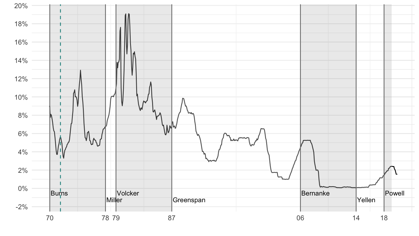
Figure 12.8: U.S. Fed Chairmen (1971-2019).
12.1 The Mundell Trilemma
According to the Mundell policy trilemma (also sometimes called impossible trinity), countries cannot have all three of the following at the same time:
- Free capital mobility,
- Monetary autonomy,
- A fixed foreign exchange rate.
Most countries (apart from China) have found free capital mobility hard to give up, and so they have resorted to the following two options:
Exchange rate targeting. A clear case is that of countries which simply give up their currency. For example, countries in the Euro area cannot have an independant monetary policy as a result. Many emerging economies (such as Turkey, Argentina) also “peg to the dollar”: they have an exchange rate target in mind.
Inflation targeting. They then have free capital mobility and monetary autonomy. For example, the U.S., the U.K., Japan, the Euro area as a whole operate under such a system. These countries usually resort to inflation targeting: they seek to attain a particular value for inflation.
Note that the distinction above is a little bit theoretical and artificial, as many countries in practice adopt a mix of the above two options:
Most inflation targeting central banks often operate with exchange rate concerns in mind, as well. For example, Donald Trump does not like when the value of the dollar fluctuates too much, especially when it is led to appreciate. Such a type of intervention is not consistent with pure inflation targeting.
On the contrary, fixed exchange rate regimes sometimes collapse, when countries realize that they would like to take back the control of their own monetary policy. (as we shall see, one reason can be to devalue to restore their competitiveness) Such was the case in Argentina in 2001, which abandoned its peg to the dollar; and Greece was very close to leaving the Euro area for the same reason.
12.2 Nominal and Real Exchange Rates
The nominal exchange rate is the price of the domestic currency in terms of foreign currency. For example, and to fix ideas, the Euro-Dollar nominal exchange rate gives the number of euros that one dollar can buy. In other words, it is the price of the U.S. currency in terms of the European currency. On November 19, 2018, this price was: \[E=0.873 \text{ Euro / Dollar.}\]
When the price of dollars in terms of euros increases, the dollar becomes more expensive, and the nominal exchange rate appreciates.
The real exchange rate, on the other hand, is the price of domestic goods in terms foreign goods. For example, the Euro-Dollar real exchange rate gives the number of European goods that U.S. goods can buy. If \(P\) is the price of a given good in U.S. dollars, then \(E \cdot P\) is a corresponding amount converted in Euros, which allows to buy \(E \cdot P/P^{*}\) goods in U.S. dollars. This real exchange rate is denoted by \(\epsilon\): \[\epsilon=\frac{E \cdot P}{P^{*}}.\]
An increase in \(\epsilon\) corresponds to an appreciation of the real exchange rate. For example, if the price of a new MacBook Pro is $2,650.90 inclusive of tax in the U.S., and the same MacBook Pro has a price equal to 2799 euros in Europe, then the real exchange rate of the U.S. dollar is given by: \[\epsilon = \frac{0.873 \cdot 2650.90}{2799}=0.827.\] This real exchange rate implies that MacBook Pros are about 17% cheaper to buy in the U.S. than in Europe (\(0.827 = 1-0.173\)). When the nominal exchange rate of the U.S. dollar goes up, the real exchange rate also goes up: the purchasing power of Americans increases. Of course, MacBook Pros are just one of many examples of goods that can be bought both in the U.S. as well as in Europe. Other goods would give different values for the real exchange rate.
The Economist’s Big Mac Index. The Economist magazine has developed a now popular gauge of real exchange rates, based on the price of Big Macs in different cities in the world, which allows to gauge the relative degree of “overvaluation” or “undervaluation” of a currency. Indeed, the Big Mac is available in a very large number of countries. For example, as John Travolta says, the French just call it “Le Big Mac”. Figure 12.9 shows the first version of this Big Mac Index. For example, the Big Mac was then worth 370 Japanese Yen, which given that the price of the Big Mac in the United States was $1.6 at the time implied that if the prices of the Big Macs were equalized across countries, then 1 dollar should have been worth 370/1.6 = 231 yens at the time. This is the column “Implied purchasing power parity of the dollar”. However, the observed yen-dollar exchange rate at the time was such that 1 dollar could in fact only buy 154 yens at the time. This implied an undervaluation of the U.S. dollar equal to \((154-231)/231=-33.3\)% of what Big Macs should have suggested it should be.
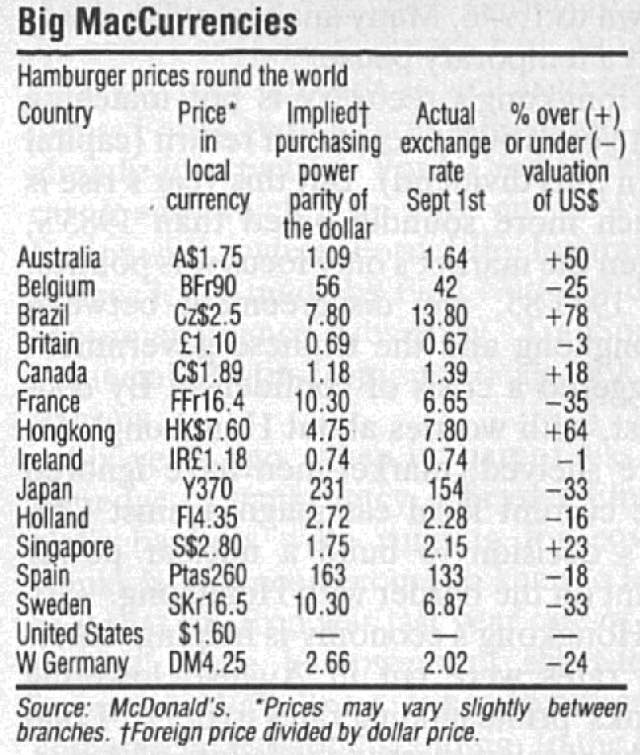
Figure 12.9: First Version of the Big Mac Index, 1986.
Table 12.1 shows more recent data for the Big Mac Index, taken from the Economist’s website.
| Country | Price | $ in Local | Price ($) |
|---|---|---|---|
| Argentina | 75.0 | 18.9 | $ 4 |
| Australia | 5.9 | 1.3 | $ 4.7 |
| Brazil | 16.5 | 3.2 | $ 5.1 |
| Britain | 3.2 | 0.7 | $ 4.4 |
| Canada | 6.5 | 1.2 | $ 5.3 |
| Chile | 2600.0 | 605.9 | $ 4.3 |
| China | 20.4 | 6.4 | $ 3.2 |
| Colombia | 10900.0 | 2844.1 | $ 3.8 |
| Costa Rica | 2290.0 | 568.5 | $ 4 |
| Czech Republic | 79.0 | 20.7 | $ 3.8 |
| Denmark | 30.0 | 6.1 | $ 4.9 |
| Egypt | 34.2 | 17.7 | $ 1.9 |
| Euro area | 4.0 | 0.8 | $ 4.8 |
| Hong Kong | 20.5 | 7.8 | $ 2.6 |
| Hungary | 864.0 | 252.1 | $ 3.4 |
| India | 180.0 | 63.9 | $ 2.8 |
| Indonesia | 35750.0 | 13359.0 | $ 2.7 |
| Israel | 16.5 | 3.4 | $ 4.8 |
| Japan | 380.0 | 110.7 | $ 3.4 |
| Malaysia | 9.0 | 4.0 | $ 2.3 |
| Mexico | 48.0 | 18.7 | $ 2.6 |
| New Zealand | 6.2 | 1.4 | $ 4.5 |
| Norway | 49.0 | 7.9 | $ 6.2 |
| Pakistan | 375.0 | 110.5 | $ 3.4 |
| Peru | 10.5 | 3.2 | $ 3.3 |
| Philippines | 134.0 | 50.7 | $ 2.6 |
| Poland | 10.1 | 3.4 | $ 3 |
| Russia | 130.0 | 56.7 | $ 2.3 |
| Saudi Arabia | 12.0 | 3.8 | $ 3.2 |
| Singapore | 5.8 | 1.3 | $ 4.4 |
| South Africa | 30.0 | 12.3 | $ 2.4 |
| South Korea | 4400.0 | 1069.2 | $ 4.1 |
| Sri Lanka | 580.0 | 153.8 | $ 3.8 |
| Sweden | 49.1 | 8.0 | $ 6.1 |
| Switzerland | 6.5 | 1.0 | $ 6.8 |
| Taiwan | 69.0 | 29.6 | $ 2.3 |
| Thailand | 119.0 | 31.9 | $ 3.7 |
| Turkey | 10.8 | 3.8 | $ 2.8 |
| UAE | 14.0 | 3.7 | $ 3.8 |
| Ukraine | 47.0 | 28.7 | $ 1.6 |
| United States | 5.3 | 1.0 | $ 5.3 |
| Uruguay | 140.0 | 28.6 | $ 4.9 |
| Vietnam | 65000.0 | 22711.5 | $ 2.9 |
It can be observed that GDP per person is a powerful predictor of the level of real exchange rates (at least according to big macs), as shown on the Table 12.2 below: richer countries have higher real exchange rates on average. You can see this when you travel: life is usually cheaper in poorer countries than in richer ones, when converted to a common currency.
| Country | Code | GDP Per Capita | Price ($) |
|---|---|---|---|
| Argentina | ARG | $ 14,592 | $ 4 |
| Australia | AUS | $ 54,066 | $ 4.7 |
| Brazil | BRA | $ 9,881 | $ 5.1 |
| United Kingdom | GBR | $ 40,361 | $ 4.4 |
| Canada | CAN | $ 45,070 | $ 5.3 |
| Chile | CHL | $ 15,037 | $ 4.3 |
| China | CHN | $ 8,759 | $ 3.2 |
| Colombia | COL | $ 6,376 | $ 3.8 |
| Costa Rica | CRI | $ 11,752 | $ 4 |
| Czech Republic | CZE | $ 20,380 | $ 3.8 |
| Denmark | DNK | $ 57,141 | $ 4.9 |
| Egypt, Arab Rep. | EGY | $ 2,440 | $ 1.9 |
| Hong Kong SAR, China | HKG | $ 46,226 | $ 2.6 |
| Hungary | HUN | $ 14,458 | $ 3.4 |
| India | IND | $ 1,981 | $ 2.8 |
| Indonesia | IDN | $ 3,837 | $ 2.7 |
| Israel | ISR | $ 40,542 | $ 4.8 |
| Japan | JPN | $ 38,332 | $ 3.4 |
| Malaysia | MYS | $ 10,254 | $ 2.3 |
| Mexico | MEX | $ 9,278 | $ 2.6 |
| New Zealand | NZL | $ 42,260 | $ 4.5 |
| Norway | NOR | $ 75,497 | $ 6.2 |
| Pakistan | PAK | $ 1,465 | $ 3.4 |
| Peru | PER | $ 6,710 | $ 3.3 |
| Philippines | PHL | $ 2,982 | $ 2.6 |
| Poland | POL | $ 13,857 | $ 3 |
| Russian Federation | RUS | $ 10,751 | $ 2.3 |
| Saudi Arabia | SAU | $ 20,804 | $ 3.2 |
| Singapore | SGP | $ 60,298 | $ 4.4 |
| South Africa | ZAF | $ 6,132 | $ 2.4 |
| Korea, Rep. | KOR | $ 29,743 | $ 4.1 |
| Sri Lanka | LKA | $ 4,105 | $ 3.8 |
| Sweden | SWE | $ 53,744 | $ 6.1 |
| Switzerland | CHE | $ 80,450 | $ 6.8 |
| Thailand | THA | $ 6,578 | $ 3.7 |
| Turkey | TUR | $ 10,514 | $ 2.8 |
| United Arab Emirates | ARE | $ 39,812 | $ 3.8 |
| Ukraine | UKR | $ 2,641 | $ 1.6 |
| United States | USA | $ 59,928 | $ 5.3 |
| Uruguay | URY | $ 16,437 | $ 4.9 |
| Vietnam | VNM | $ 2,366 | $ 2.9 |
This positive relationship between GDP per capita and Big Mac prices when converted in dollars, is plotted on Figure 12.10 below.
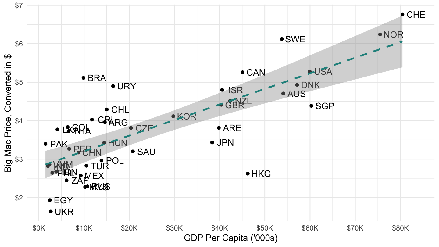
Figure 12.10: Big Mac Index and GDP Per Capita, January 2018.
12.3 Multilateral Exchange Rates
In practice, trade is not bilateral, which complicates somewhat the measurement of real exchange rates, and the assessment of competitiveness. Multilateral exchange rates require data on the geographic composition of different country’s trades, in order to properly weight different exchange rates.
12.4 Uncovered Interest Parity
The uncovered interest parity relation is based on the assumption that capital can move freely. If this is so, then investors need to be indifferent between investing in the country’s financial assets, at interest rate \(i_t\), or in the foreign country’s financial assets, at interest rate \(i_t^{*}\).
For concreteness, and to fix ideas, consider a U.S. investor’s decision thinking about holding U.S. one year bonds yielding \(i_t\) or U.K. one-year bonds yielding \(i_t^{*}\) instead. Arbitrage implies: \[1+i_{t}=\left(E_{t}\right)\left(1+i_{t}^{*}\right)\left(\frac{1}{E_{t+1}^{e}}\right)\quad\Rightarrow\quad\boxed{1+i_{t}=\left(1+i_{t}^{*}\right)\frac{E_{t}}{E_{t+1}^{e}}},\] which is called the uncovered interest parity relation or the interest parity relation. This arbitrage relationship comes from trading off the following two options, which therefore must have the same returns:
investing in the home country’s bonds at interest rate \(i_t\). One dollar then yields \(i_t\).
or alternatively, converting this dollar into pounds at exchange rate \(E_t\) (\(E_t\) is indeed the number of pounds per dollar, for example if $1 = £0.91 then \(E_t=0.91\)), investing it in U.K. bonds, earning interest rate \(i_t^{*}\), and then converting it back into dollars. With \(E_t \cdot (1+i_t^{*})\) pounds, one expects to get \(E_t \cdot (1+i_t^{*})/E_{t+1}^e\) dollars. Indeed, \(1/E_t\) is the number of dollars per pound. For example if $1 = £0.91, then £1 \(\approx\) $1.10 and \(1/E_t=1.10\). \(1/E_{t+1}^e\) is the expected value of that exchange rate at time \(t+1\), which allows to convert pounds into dollars.
Assuming that expectations of future exchange rates are fixed at a certain level so that \(E_{t+1}^e = \bar{E}\), then this equation implies that: \[\boxed{E_{t}=\frac{{1+i_{t}}}{1+i_{t}^{*}}\bar{E}}.\]
Therefore:
when the nominal interest rate goes up, the nominal exchange rate appreciates.
when the nominal interest rate goes down, the nominal exchange rate depreciates.
As a consequence, the uncovered interest parity equation explains why an easing of monetary policy (lowering of interest rates \(i\)) leads to a depreciation of the currency, while a tightening of monetary policy (increase in interest rates) leads to an appreciation of the currency. To the extent that in the short run, movements of real exchange rates are largely determined by the movements of nominal exchange rates, we can understand how monetary policy can influence the level of real exchange rates. In turn, this impacts the competitiveness of its exports, and therefore potentially increases aggregate demand through the boost to net exports \(NX\).
This relation also implies that if exchange rates are fixed, so that \(\bar{E}_t=\bar{E}\), then interest rates need to be equalized across countries, or capital would move to the highest interest rate (remember, we assume free mobility of capital). Therefore: \[\boxed{\bar{E}_t=\bar{E} \quad \Rightarrow \quad i_t = i_t^{*}}.\]
This implies that countries who want to fix their exchange rate, cannot have an independant monetary policy. The interest rate that they set needs to be the same as whichever countries they are fixing their exchange rate to. (this is a good depiction of emerging markets which peg their exchange rates to the dollar)
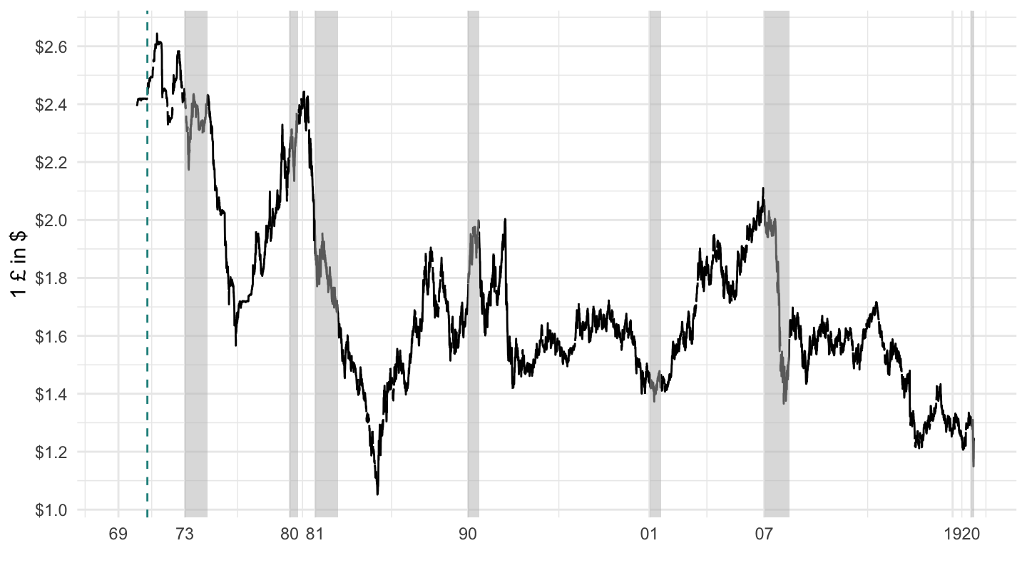
Figure 12.11: U.S. - U.K Nominal Exchange Rate
Figure 12.12 plots the number of dollars which can be bought by one euro from 1999 to 2019, or the number of dollars which can be bought by 1.95583 deutschmarks in the period from 1970 to 1999 (since it was decided that 1 € = 1.95583 DEM in 1999).
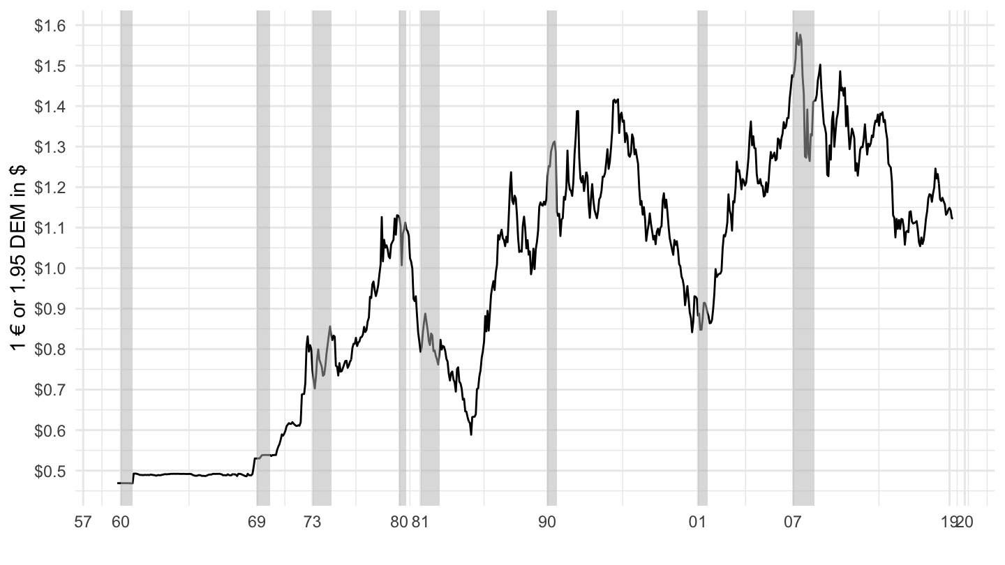
Figure 12.12: U.S. - Euro Nominal Exchange Rate
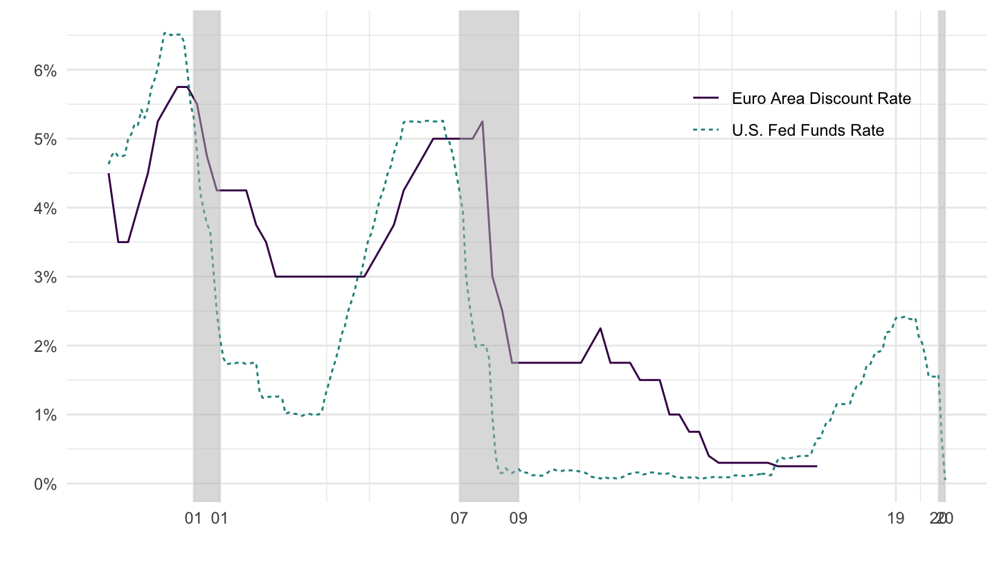
Figure 12.13: U.S. Versus Euro Area Discount Rates
12.5 Some Data
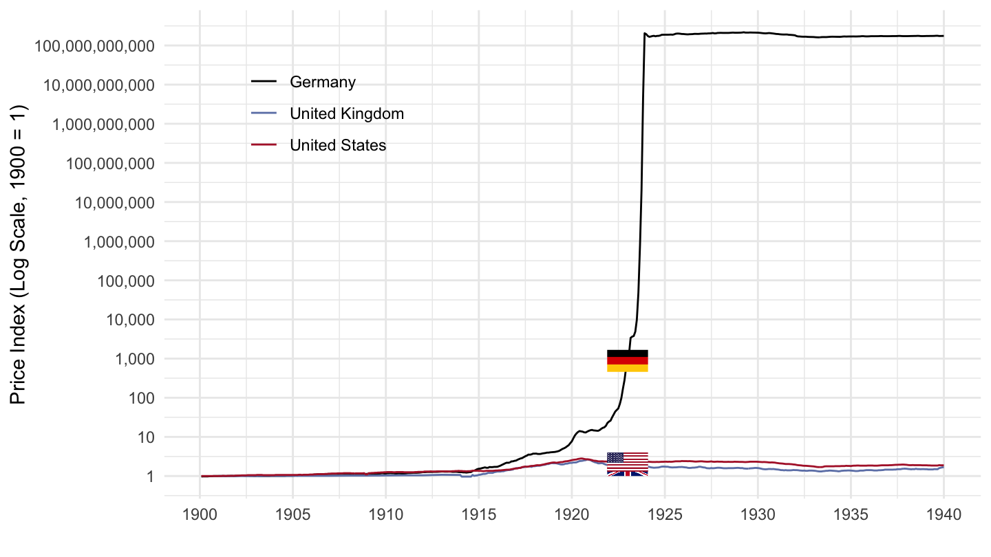
Figure 12.14: Hyperinflation in Germany (1900-1940)
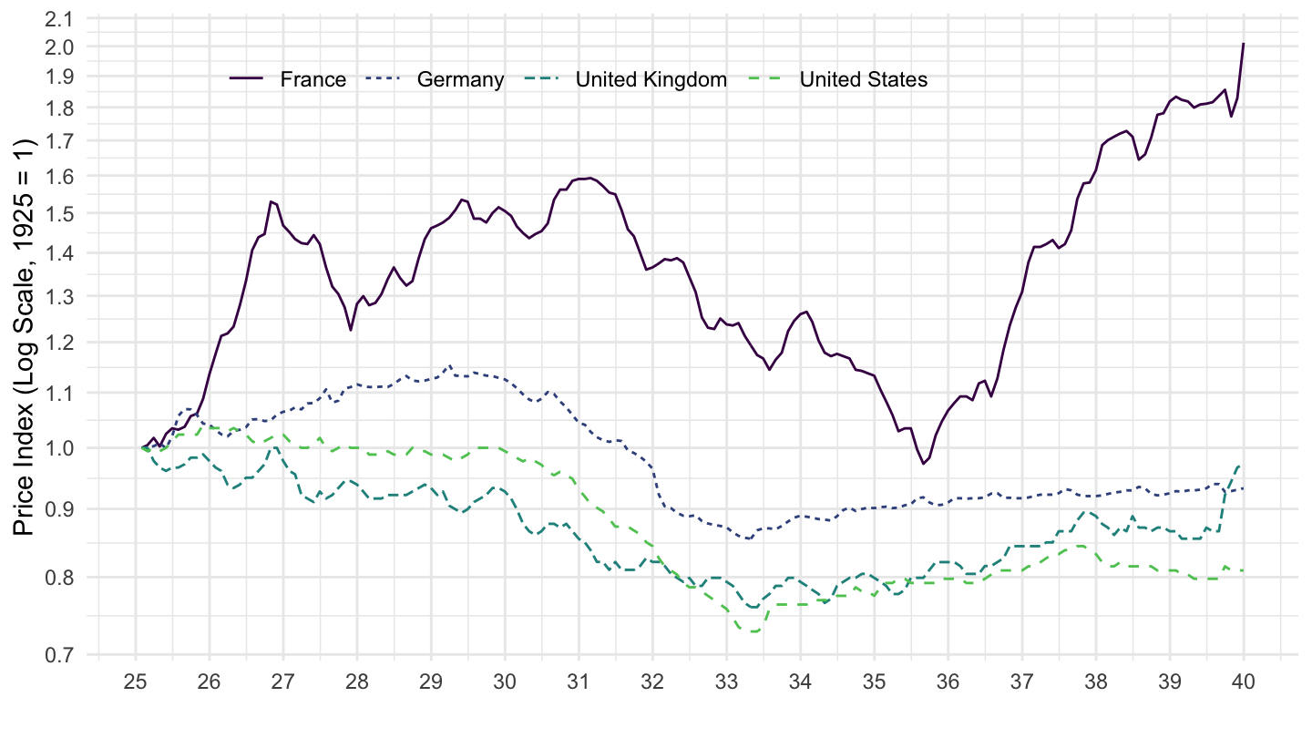
Figure 12.15: Deflation during the Great Depression
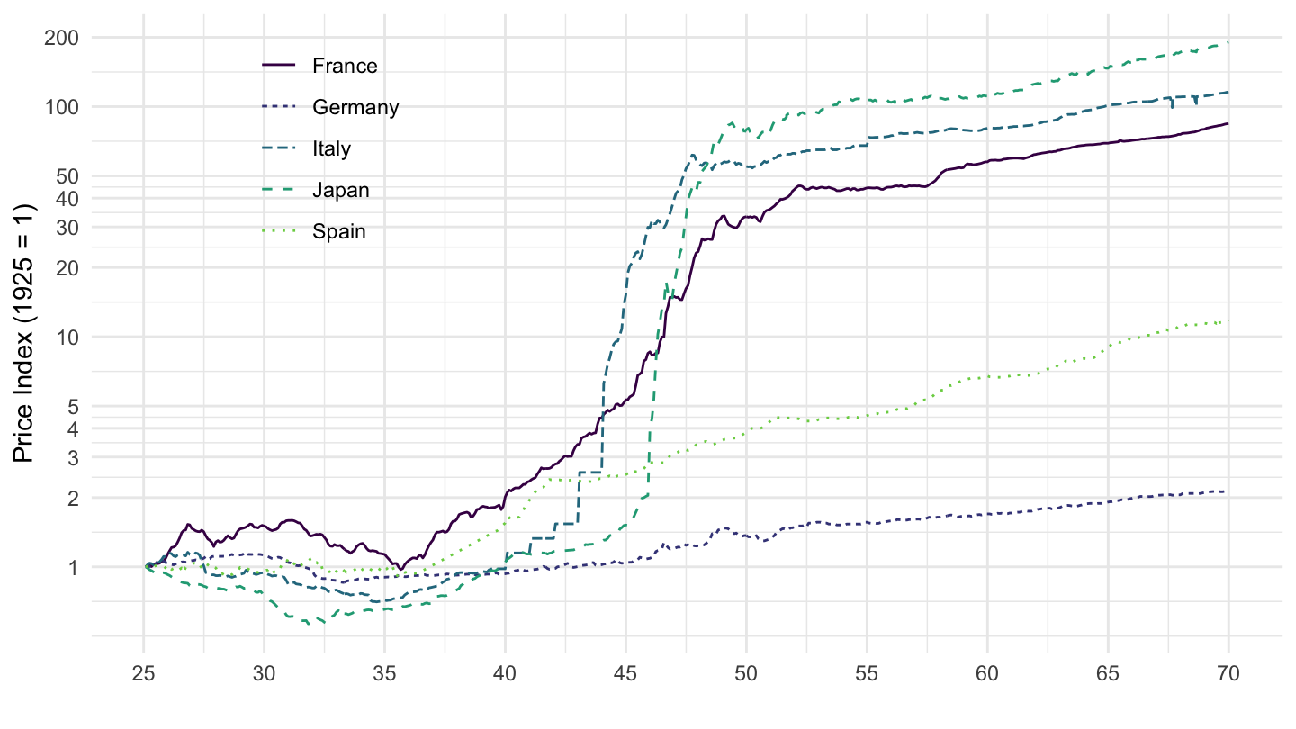
Figure 12.16: Inflation in Italy, Japan, Spain, and Switzerland (1925-1970)
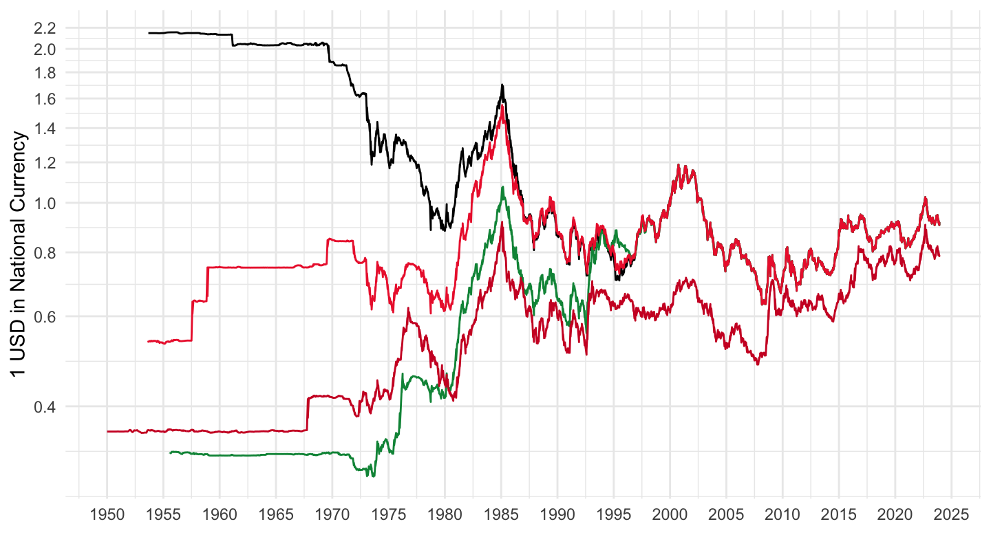
Figure 12.17: Exchange Rates against US. Dollar (1950-2020)
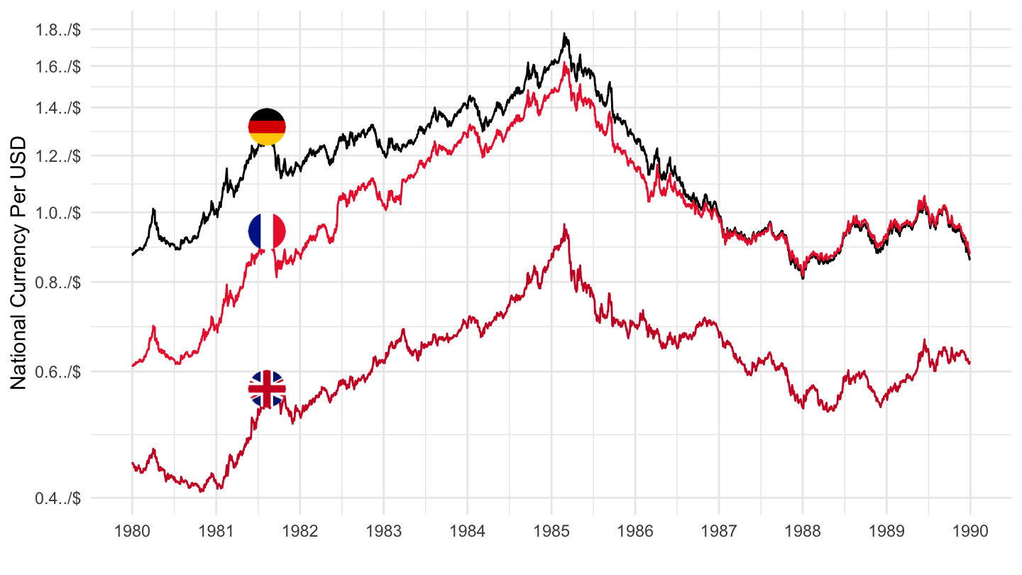
Figure 12.18: Exchange Rates around Plaza Accords (1980-1990)
Figure 12.19: Plaza Accords.
12.6 The Credit Channel
Another very important channel through which monetary policy works is through its effect on the U.S. mortgage markets. There is no better example of this than the last financial crisis.
In the U.S. and in the U.K., many homeowners borrow at a rate close to the rate set by the Federal Reserve. There are two ways through which monetary policy potentially affects aggregate demand of households:
With adjustable rate mortgages, the payments of these borrowers with a mortgage automatically follow short term interest rates. When interest rates go up, these payments increase. When interest rates go down, these payments de decrease.
Even with fixed rate mortgages, most households may refinance their loans when interest rate go down; which provides a powerful potential stimulative effect of monetary policy. Indeed, refinancing then allows them to reduce their mortgage payments and increase disposable income. Of course, creditors lose on the other side, but they tend to have much lower marginal propensities to consume.
The Federal Funds Rate were kept low for a very long time between 2000 and 2004 as shown on Figure 12.20 (Alan Greenspan was then Chairman of the Federal Reserve, from 1987 to 2006), which led to a lot of refinancing activity, and helped boost consumption.
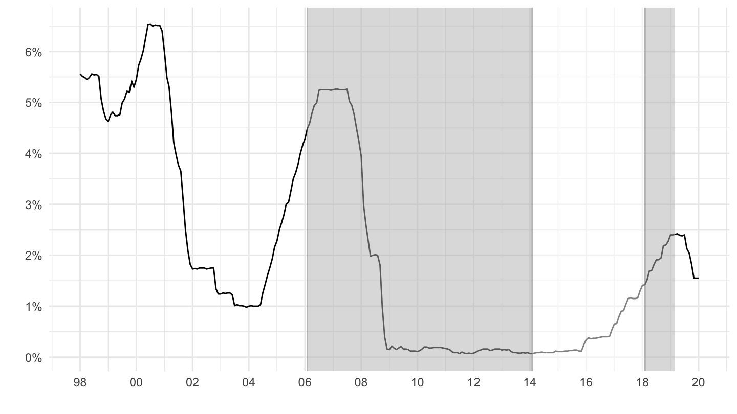
Figure 12.20: Low Federal Funds Rates.
It also led to the buying of many new homes. Many new homeowners were taking on loans at very low interest rates, not realizing that they would not be able to repay them when the Federal Reserve would move interest rates back up. Figure 12.22 shows that many delinquent borrowers during the crisis had indeed taken these adjustable rate mortgages. Starting in 2004, the Federal Reserve started raising interest rates, which increased the mortgage payments to households whose mortgages were reset. Some of them could not make these payments, and so had to default. Adding to the consumption boom was the fact that many homeowners were using “homes as ATMs”, in the sense that cash-out refinancing allowed them to extract cash from rising house prices (see Figure 12.23). Figure 12.24 shows how unprecedented the run up in house prices was.
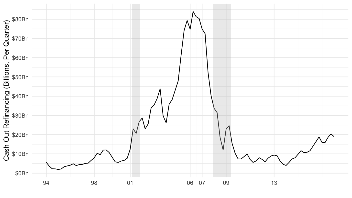
Figure 12.21: Quarterly Cash-Out Refinancing Volumes (1995-2019). Source: Freddie Mac.
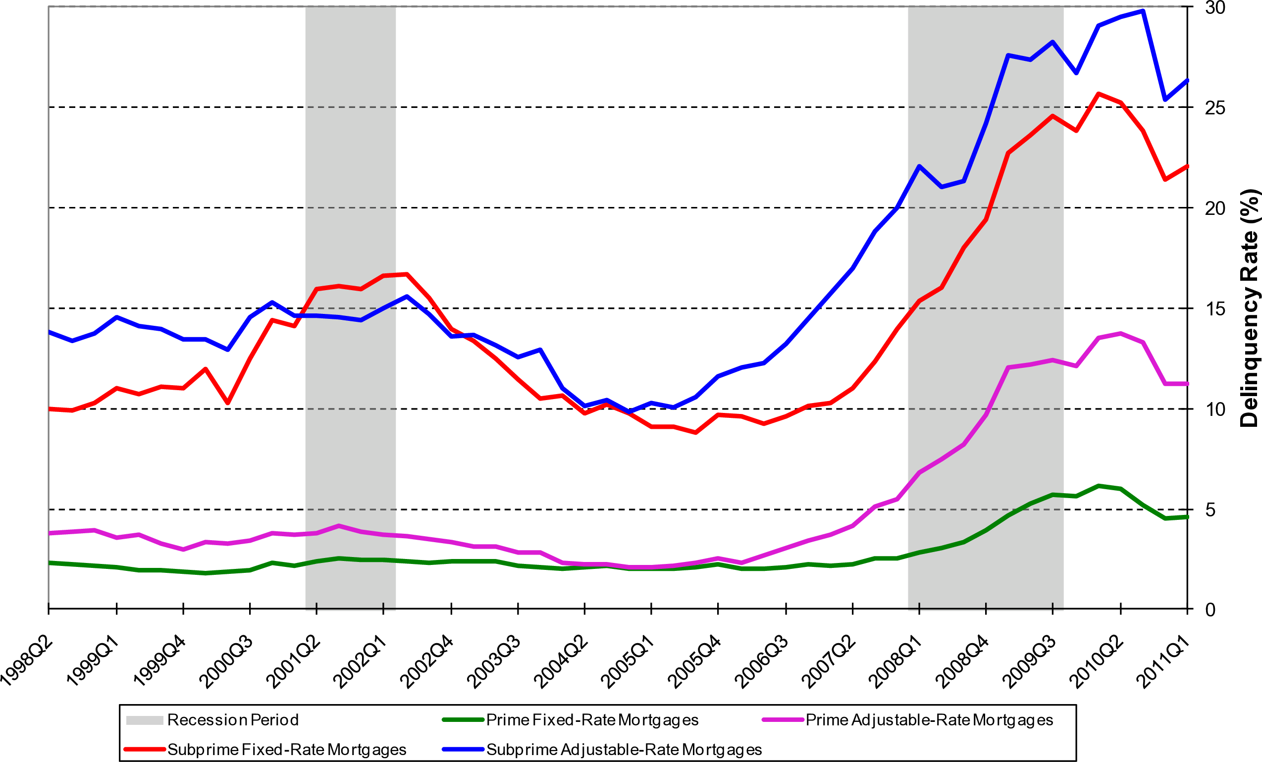
Figure 12.22: Delinquency Rates on Mortgages: Prime, Subprime, Adjustable, Fixed. Source: Richmond Fed.
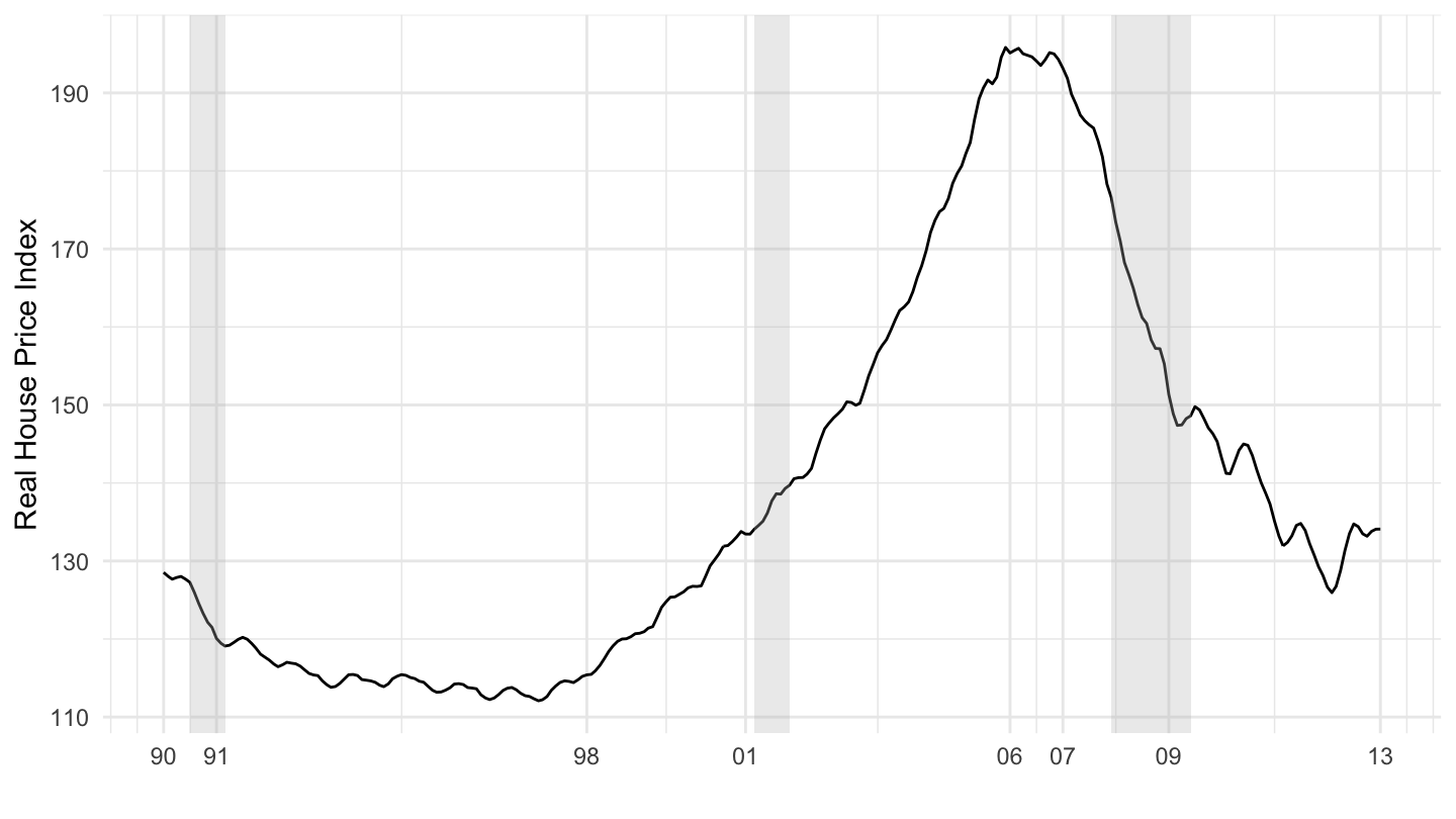
Figure 12.23: U.S. Real House Prices (1990-2013). Source: Shiller.
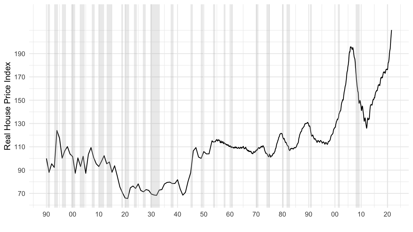
Figure 12.24: U.S. Real House Prices (1890-2019). Source: Shiller.
One factor was one of the Keynesian feedback effect we have been studying all along. Lower disposable income coming from rising interest rates led to lower aggregate demand, which increased unemployment, causing further declines in incomes, which in turn led to more bankruptcies, in a vicious cycle.
Michael Burry, a former UCLA undergraduate, saw it coming. Please watch his commencement speech on Figure 12.25 before the next lecture.
Figure 12.25: Michael Burry’s 2012 UCLA Commencement Speech.
Required Readings
(Required Watching) Adam McKay. The Big Short. 2015.
Michael J. Burry, “I Saw the Crisis Coming. Why Didn’t the Fed?”, The New York Times, April 4, 2010.
“Two out of three ain’t bad.” The Economist, August 27, 2016.
“Should egalitarians fear low interest rates?”, The Economist, July 11, 2019.