5 Technological Progress
Link to slides / Link to handouts
In this lecture, we start by reviewing some facts on long-run economic growth in section 5.1. We then review an endogenous growth model 5.6 which tries to account for long-run economic growth.
5.1 Long-run Economic Growth
In this section, we remind ourselves some basic facts on technological growth since the 1200s. We in particular use Angus Maddison’s long run data series on GDP per capita in major advanced economies, to show that growth as we know it is a rather recent phenomenon, one that starts at the beginning of the nineteenth century.
The Figures below show GDP per capita in France, Germany, Italy, the United Kingdom, and the United States, starting respectively in 1200, 1700, 1800, and 1900. These are presented on a semi-logarithmic scale (that is, the y-axis is in log), also sometimes called a ratio scale. Do not worry too much about the unit in which GDP per capita is expressed in this Maddison data: the unit is called the Geary–Khamis dollar, but we shall come back to it when we discuss the issue of real exchange rates and purchasing power parity comparisons. The reason for using such a semi-logarithmic scale is that growth is roughly exponential, so it is approximately linear on a semi-logarithmic scale.
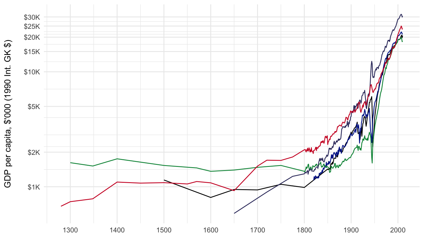
Figure 5.1: 1200-2010 GDP per capita (Maddison Data).
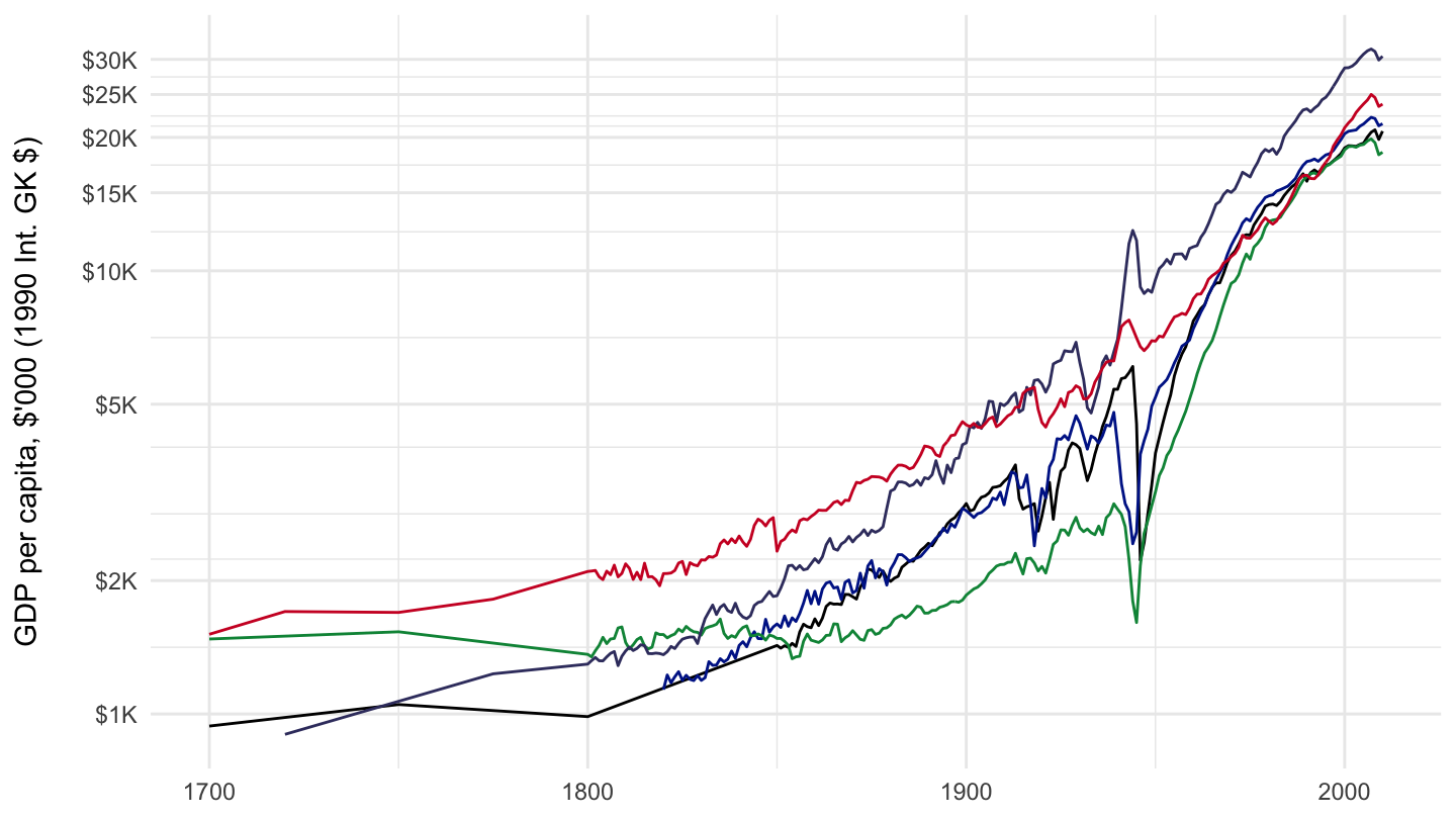
Figure 5.2: 1700-2010 GDP per capita (Maddison Data).
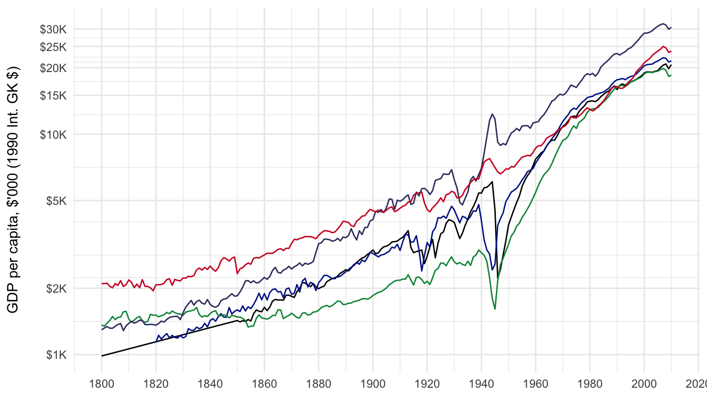
Figure 5.3: 1800-2010 GDP per capita (Maddison Data).
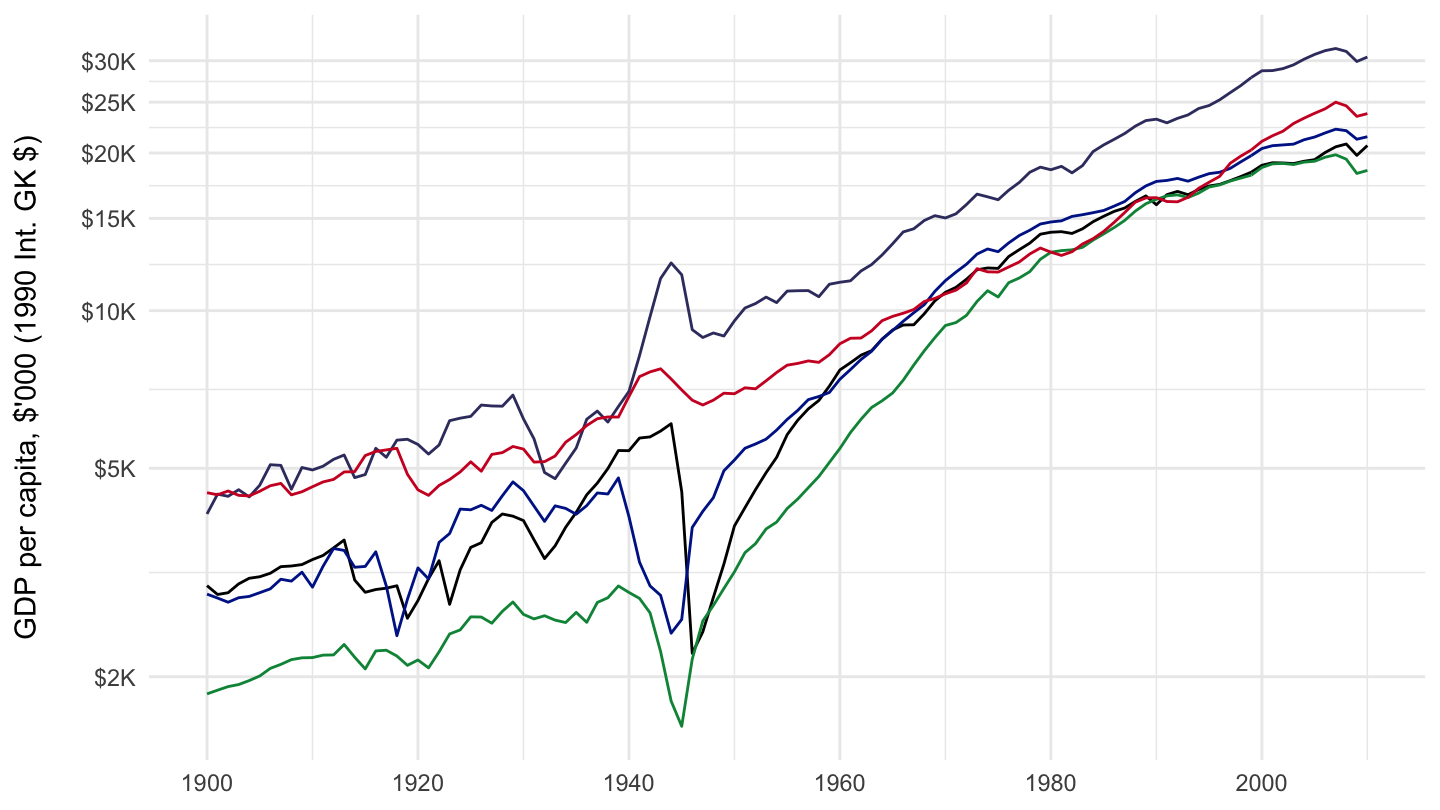
Figure 5.4: 1900-2010 GDP per capita (Maddison Data).
5.2 The Mathematics of Growth
The mathematical orders of magnitude with exponential growth are sometimes hard to grasp intuitively. This section provides you with some maths to help get an intuitive feel for exponential growth. Let’s consider an economic quantity \(y_t\), growing at a constant rate \(g\). For our purposes in this lecture, \(y_t\) is GDP per capita, but it could also veru well be a price level, consumption, or some other economic quantity. Iterating on the difference equation allows to get \(y_t\) as a function of the initial value: \[ \begin{aligned} y_t = (1+g)y_{t-1} \quad \Rightarrow \quad y_t = (1+g)^t y_0. \end{aligned} \] How fast of a growth is that? The number of years \(T\) it takes for GDP per capita to be multiplied by a factor \(F\) (where \(F=2\), if we are looking for GDP to double) is given by : \[ \begin{aligned} &y_t = F y_0 \quad \Rightarrow \quad (1+g)^t y_0 = F y_0 \quad \Rightarrow \quad (1+g)^T = F \\ & \quad \Rightarrow \quad \ln (1+g)^T = \ln F \quad \Rightarrow \quad T \ln (1+g) = \ln F \\ & \quad \Rightarrow \quad T=\frac{\ln F}{\ln(1+g)}. \end{aligned} \] For small rates of growth, we know that a Taylor expansion of the \(\ln\) gives \(\ln(1+g)=g\), so that this formula can be approximated by: \[T = \frac{\ln F}{g}.\]
Rule of 70. This formula gives the “rule of 70” for small growth rates. The “rule of 70” states that a quantity which grows at a rate \(g\) in percentage terms, takes approximately \(70/g\) years to double. This comes from the fact that \(100*ln(2) \approx\) 69.3147181. For example, if GDP per capita is growing at 2% per year, then it takes approximately 35 years for it to double: approximately one generation only. If it is growing at 1% per year, it takes approximately 70 years for it to double, so two generations. Whether you grow to be twice as rich as your parents, or twice as rich as your grandparents on average makes a big difference.
Rule of 230. The same formula also gives the “rule of 230” for small growth rates. The “rule of 230” states that a quantity which grows at a rate \(g\) in percentage terms, takes approximately \(230/g\) years to be multiplied by \(10\). This is because: \(100*ln(10) \approx\) 230.2585093. Thus, with a 2% growth rate, GDP per capita is multiplied by \(10\) over (as an exercise, you may create your own rules…)
5.3 Questions
Section 5.1 has shown that economic growth has been 2% on average in advanced economics, in the last two centuries. This raises a number of questions.
Why is there GDP per capita growth at all? One major shortcoming of Bob Solow’s Growth model of lecture 1.5 and of Peter Diamond’s growth model of lecture 4 is that they fail to account for long run economic growth - rather ironically. According to these models, the process of capital accumulation reaches a steady-state at some point, such that capital per capita, GDP per capita, remain forever constant. This happens for intuitive reasons: if the labor force is given, then growth cannot be sustained through capital accumulation alone. In fact, in the Solow model, even a saving rate equal to 100% would lead to very high GDP, but not to constant GDP growth. At one point, the capital stock would be so large that merely maintaining it would consume all output. Output would then be equal to gross saving, and depreciation. This is coming from the fact that at the steady state of the Solow model, gross saving is given by \(s Y^{*}\) which would then be equal to \(Y^{*}\) (if \(s=1=100\%\)), which is also equal to depreciation as: \[s Y^{*}=\delta K^{*}.\]
The Cross-section of Countries: Rich versus Poor Countries. The power of compounding is such that even a few decades of lower growth makes a big difference. Given persistent differences in growth rates, per capita GDP is far from being equalized across countries. Contrary to the predictions in the Solow growth model, there has hardly been a strong catch up of poor countries towards the level of rich countries. On one hand of the spectrum, many countries have very small GDP per capita levels.
| Country | GDP per capita |
|---|---|
| Ethiopia | $ 1,489 |
| Togo | $ 1,446 |
| Sierra Leone | $ 1,353 |
| Guinea-Bissau | $ 1,257 |
| Madagascar | $ 1,237 |
| Mozambique | $ 1,211 |
| D.R. of the Congo | $ 1,199 |
| Malawi | $ 971 |
| Liberia | $ 877 |
| Niger | $ 868 |
| Burundi | $ 840 |
| Central African Republic | $ 599 |
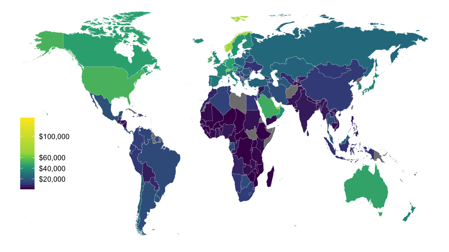
Figure 5.5: 2014 GDP per capita, by Country (Penn World Tables).
On the other, some countries have very high GDP per capita. Table 5.2 below shows the countries that have a GDP per capita higher than $40K.
| Country | GDP per capita |
|---|---|
| Qatar | $ 146,037 |
| China, Macao SAR | $ 130,758 |
| Norway | $ 75,920 |
| United Arab Emirates | $ 68,021 |
| Kuwait | $ 67,432 |
| Brunei Darussalam | $ 66,968 |
| Singapore | $ 66,050 |
| Luxembourg | $ 65,842 |
| Switzerland | $ 61,570 |
| United States | $ 51,623 |
| Ireland | $ 51,224 |
| Netherlands | $ 47,392 |
| Saudi Arabia | $ 46,772 |
| Germany | $ 46,190 |
| China, Hong Kong SAR | $ 45,399 |
| Austria | $ 45,158 |
| Denmark | $ 43,733 |
| Australia | $ 43,590 |
| Canada | $ 42,794 |
| Sweden | $ 42,117 |
| Taiwan | $ 41,514 |
Why are poor countries so poor, and largely failing to catch up, and why advanced economies are growing at an average of 2% per year since the beginning of the nineteenth century, are perhaps the potentially most impactful questions for economics, but also those for which economists perhaps know the least. This lecture presents an attempt at endogenizing GDP per capita growth, based on the a very simplified version of Paul Romer’s endogenous growth model. This may allow us to shed light on some of these issues.
5.4 Objects VS Ideas
A crucial distinction for understanding endogenous growth theory, is that of objects versus ideas.
Objects. Objects like houses, food, or cell phones are rivalrous. That is, one person’s use of one of these particular objects prevents its use by someone else. Most goods are rivalrous, and this is what leads to scarcity, the central topic of economics.
Ideas and recipes. In contrast, ideas are nonrival. My use of an idea does not prevent someone else’s use of that idea. For example, after it has been shot, a movie can be shown in any theatre in the world, and for a cost equal to zero on the internet (apart for the cost of electricity, and of storing the movie on servers). Similarly, a recipe for a pharmaceutical drug takes years to develop. However, once the drug has been invented, the cost of producing this drug is typically very small, much smaller than the associated initial fixed cost. Finally, Antonín Dvořák’s 9th Symphony “From the New World” can be performed by any orchestra in the world, Gustavo Dudamel’s or Herbert Von Karajan’s, once Antonín Dvořák has composed it.
According to Paul Romer, ideas and recipes have the potential to be a source of indefinite economic growth:
Every generation has perceived the limits to growth that finite resources and undesirable side effects would pose if no new recipes or ideas were discovered. And every generation has underestimated the potential for finding new recipes and ideas. We consistently fail to grasp how many ideas remain to be discovered.
As Chad Jones puts it describing Paul Romer’s contributions in a Vox Eu article:
Once you’ve got increasing returns, growth follows naturally. Output per person then depends on the total stock of knowledge; the stock doesn’t need to be divided up among all the people in the economy. Contrast this with capital in a Solow model. If you add one computer, you make one worker more productive. If you add a new idea – think of the computer code for the first spreadsheet or word processor or even the internet itself – you can make any number of workers more productive. With non-rivalry, growth in income per person is tied to growth in the total stock of ideas – an aggregate – not to growth in ideas per person.
However, ideas implies increasing returns and therefore, potentially inefficient market outcomes.
5.5 Increasing Returns
Because of increasing returns, a competitive market economy may not lead to an efficient level of development of ideas. The issue with pure competition is that if a movie director was forced to charge a price equal to the marginal cost of showing a movie, then he would have to charge a zero price for this movie, as it would then be available for everyone to watch on Youtube. Similarly, once a drug against AIDS (for example) has been invented, one would ideally like to give this drug to the largest possible number of people. Indeed, the marginal cost of producing a new drug is much lower than the cost at which it is commercialized. However, this would decrease the incentives to innovate in the first place.
Patents. One way that this market failure has historically been addressed, is by granting patents (property rights) on newly invented ideas. (in biology, scientists are sometimes granted 12 years of exclusivity; in chemistry, they may be granted 5 years) Similarly, intellectual property rights, as well as laws against piracy, have the same purpose: they seek to encourage innovation by preventing 0 marginal cost pricing. Note however that patents should not be too strong either, or they discourage the use of new ideas, potentially at a suboptimal level. In fact, historically, especially in periods of high innovation and economic growth, intellectual property rights were relatively weak. When the US was a rising economic power, it was also a notorious pirate of intellectual property, very much like what China is being accused of today.
Government funded research. One alternative way through which R&D can be incentivized, while allowing for large dissemination, is to have the allow for government funded research. For example, the Department of Defense’s ARPANET was a precursor of today’s World Wide Web.
Prizes. Another way for the government to incentivize fundamental research is to give out prizes, which are a rather inexpensive way to motivate researchers hoping for recognition. The Economics Nobel Prize is one such example. In general, the motivations of researchers are complex, and probably not purely driven by profit seeking. For example, a very large community of developers contributes to open-source software, which is hard to rationalize from an orthodox (individualist) economic standpoint.
5.6 Endogenous Growth Model
Paul Romer was awarded the Nobel Prize in Economic Sciences last year. The Economist is a good coverage of his work. In this section, we present a very simplified version of his much more subtle ideas.
Model. In Paul Romer’s endogenous growth model, there are two types of workers: research workers, whose number is \(L_{at}\), and production workers, whose number is \(L_{yt}\). We denote the share of research workers in total labor by \(l\), so that: \[L_{at} = l L\] The number of production workers is simply the complement of that, so that: \[L_{yt} = (1-l)L.\] As an example, if \(l=0.10\), then 10% of the labor force works in the R&D sector. For simplicity, we neglect the role of capital and capital accumulation, an issue that you will take up during sections. Therefore, production is simply given by: \[Y_{t} =A_{t} L_{yt}\]
Finally, productivity is assumed to grow at a rate that is function of the productivity of the research sector \(z\), overall productivity \(A_t\), and the number of researchers in the research sector \(L_{at}\): \[\Delta A_{t+1} =z A_{t} L_{at}.\]
Solution. In order to solve this model, we may simply iterate on the production function for new ideas, as a function of the initial value for productivity \(A_0\) (just as there was an initial value for capital \(K_0\) in the Solow growth model), and using that the number of research workers is \(L_{at} = l L\): \[ \begin{aligned} & \Delta A_{t+1} = A_{t+1}-A_t =z A_{t} L_{at}\\ & \quad \Rightarrow \quad A_{t+1} = (1+z L_{at})A_{t} \\ & \quad \Rightarrow \quad A_{t+1}=\left(1+zlL\right)A_{t}\\ & \quad \Rightarrow \quad A_{t}=\left(1+zlL\right)^{t}A_{0}. \end{aligned} \] Replacing then \(L_{yt}\) in the production function with \(L_{yt} = (1-l)L\), as well as this endogenous level of productivity, we get: \[ \begin{aligned} Y_{t}& =A_{t} L_{yt}\\ &= \left(1+zlL\right)^{t}A_{0}L_{yt}\\ &= \left(1+zlL\right)^{t}A_{0}(1-l)L\\ Y_{t}&= A_{0}(1-l)L \left(1+zlL\right)^{t} \end{aligned} \]
Change in \(l\). A change on the research share of workers has too opposing effect. On the one hand, there are less production workers available for production Thus, there is a fall in \(L_{yt}\), which tends to reduce \(Y_t\). On the other, overall growth, which is here given by \(g = zlL\), is then permanently higher.
5.7 Shortcomings
In Paul Romer’s model, all economic growth comes from R&D. Despite its successes, this model however leaves a number of questions unanswered. For example, it is unclear why poor countries are not able to benefit from “ideas” which are available in rich countries. Ideas being a public good, they are potentially available for anyone to use. Then, productivity \(A_t\) should be quite similar in rich and poor countries. Moreover, the endogenous growth model does not really explain why economic growth took off where and when it took off (in the UK, at the beginning of the nineteenth century), a question we started out with.
If you want to know more, this Economist article gives a number of limitations on the theory of economic growth. In particular, economic historians are still debating the origins of the Industrial Revolution. Important factors that the endogenous growth model neglects are the relative importance of secure property rights, the extent to which cultures tolerate personal ambition, and other cultural or political factors, all of which certainly matter for economic growth. You may refer to the next section, if you wish to read more about economic growth.
Additional Readings
Chad Jones, New ideas about new ideas: Paul Romer, Nobel laureate, Vox Eu, October 12, 2018.
Paul Krugman, Notes on Global Convergence (Wonkish and Off-Point), New York Times, October 20, 2018.
(Gated) Time to fix patents, The Economist, August 8 2015.
(Gated) A question of utility, The Economist, August 8, 2015.
(Gated) Economists understand little about the causes of growth, The Economist, April 12, 2018.
(Gated) Paul Romer and William Nordhaus win the economics Nobel, The Economist, Oct 13, 2018.