11 Open Economy

Link to slides / Link to handouts

In the previous lectures, we have maintained that the economy was closed, a strong and unrealistic assumption. This assumption can only be justified when thinking about the world as a whole. However, the relevance of the theory is then considerably diminished, because fiscal policy such as government spending or the tax and transfer system, are largely decided at the national level.

One key idea of today’s lecture is that in an open economy, Keynesian stimulus is less efficient, which is all the more true when the economy is more open. This result is intuitive: in an open economy, some of the increased aggregate demand by consumers is addressed to foreign products. J.M. Keynes describes this phenomenon in The General Theory of Employment, Interest and Money as follows:

In an open system with foreign-trade relations, some part of the multiplier of the increased investment will accrue to the benefit of employment in foreign countries, since a proportion of the increased consumption will diminish our own country’s favourable foreign balance; so that, if we consider only the effect on domestic employment as distinct from world employment, we must diminish the full figure of the multiplier. On the other hand our own country may recover a portion of this leakage through favourable repercussions due to the action of the multiplier in the foreign country in increasing its economic activity.

During this lecture, we will extend the extended goods market model of lecture 9 to allow for the importing and exporting of goods, as well as the potential for a deficit or a surplus in the trade balance $NX$. We will show that the value for the Keynesian multiplier is then reduced, all the more so that the economy is open.

Very importantly, you should not necessarily think of the economies we consider here as countries. States, counties, or even zipcodes, also are open economies (which share a fixed exchange rate with respect to other states, counties, or zipcodes). Thus, the model is applicable if, for example, California decides to engage in fiscal stimulus (by lowering state taxes, for instance). Of course, California is much more open than the U.S. as a whole, as California imports many products from other states (a quarter of its electricity, for example), and exports many products to other states (such as Google, Apple, or Facebook). Therefore, we shall see that California has much less power than the U.S. as a whole to stimulate aggregate demand.

11.1 Neoclassical Model with Traded and non-Traded Goods

We first consider a neoclassical model with full employment, where there are two types of goods: a non-traded good denoted by $N$ and a traded good denoted by $T$. This model is therefore often called the T/NT model (sometimes, in textbooks you might run into $NT$ that denotes non-traded goods instead of $N$). We normalize the traded goods’s price to $p_T = 1$. The relative price of non-traded goods is given by $p_N$ (in your microeconomics class, you would run with $p_N/p_T$ instead).

Supply. Assume that non-traded goods, and traded goods are produced with decreasing returns to scale, and productivities $A_N$ and $A_T$: \[y_N = A_N l_N^{1-\alpha} \qquad \text{and} \qquad y_T = A_T l_T^{1-\beta},\] where $l_N$ is labor demand in the non-traded goods sector, and $l_T$ is labor demand in the traded goods sector, with: \[l_N + l_T = l.\]

In a neoclassical model, the wage is the same in the traded and in the non-traded goods sector, because non-traded goods firms maximize: \[\max_{l_N} \quad y_N - w l_N \quad \Rightarrow \quad w = (1-\alpha)p_N A_N l_N^{-\alpha}\]

and traded goods firms maximize: \[\max_{l_T} \quad y_T - w l_T \quad \Rightarrow \quad w = (1-\beta)A_T l_T^{-\beta}\]

Therefore: \[\boxed{p_N = \frac{1-\beta}{1-\alpha}\frac{A_T}{A_N}\frac{l_N^{\alpha}}{(l-l_N)^\beta}}\]

Demand. Assuming an elasticity of substitution equal to $\gamma$ across the consumption of traded $c_T$ and the consumption of non-traded goods $c_N$: \[ \begin{aligned} \max_{c_{T}, c_{N}} & \quad \omega_{T}^{\frac{1}{\gamma}} c_{T}^{\frac{\gamma-1}{\gamma}}+\left(1-\omega_{T}\right)^{\frac{1}{\gamma}} c_{N}^{\frac{\gamma-1}{\gamma}}\\ &\text{s.t.} \quad c_{T} + p_{N} c_{N} = w + \text{profits}. \end{aligned} \]

Instead of “consumption today”, and “consumption tomorrow”, we here have two goods in the same period. Again, there are four methods to show that: \[\frac{(1-\omega_T)^{\frac{1}{\gamma}}c_{N}^{-\frac{1}{\gamma}}}{\omega_T^{\frac{1}{\gamma}}c_{T}^{-\frac{1}{\gamma}}} = p_{N} \quad \Rightarrow \quad p_N = \left(\frac{1-\omega_T}{\omega_T}\right)^{1/\gamma} \left(\frac{c_{T}}{c_{N}}\right)^{1/\gamma}.\]

Denoting by $b$ the trade deficit (which corresponds to exports of traded goods), we get: \[\boxed{p_N = \left(\frac{1-\omega_T}{\omega_T}\right)^{1/\gamma} \left(\frac{A_T(l-l_N)^{1-\beta} + b}{A_N l_N^{1-\alpha}}\right)^{1/\gamma}}\]

Examples. If the formulas above seem a bit complicated to your taste, then there are various special cases that allow us to build intuition around the model.

Constant returns. Assuming constant returns in the production of non-traded goods, and traded goods leads to the following : \[\alpha = \beta = 0 \quad \Rightarrow \quad p_N=\frac{A_T}{A_N}.\]
Inelastic demand. Assuming $\gamma = 0$, that is assuming inelastic demand in the consumption of traded and non-traded goods (that is, assuming that one wants to consume fixed proportions of traded and non-traded goods), we get that $l_N$ is just fixed as a function of $p_N$, so that the demand equation is simply: \[\frac{A_T(l-l_N)^{1-\beta} + b}{A_N l_N^{1-\alpha}} = \frac{\omega_T}{1-\omega_T}.\]

11.2 Aggregate Demand in the Open Economy

In this lecture, we shall abstract from exchange rate considerations altogether (in terms of the notations which we shall introduce later, $\epsilon=1$):

A literal way to interpret this assumption is to assume that exchange rates are fixed. This would be the case if a country has a fixed exchange rate regime vis-a-vis the rest of the world. This situation describes well Euro-area countries which share a common currency, or countries which peg their currencies to the dollar. This situation also describes the Gold Standard regime, or the “gold-exchange standard” Bretton Woods system before the Nixon Shock, when direct convertibility of the U.S. dollar to Gold was suspended.
Even if exchange rates are not fixed, we can already learn a lot by focusing on quantities (export and import volumes), and abstracting from exchange rates for now. We shall discuss exchange rate policy during some of the next lectures. In particular, even though exports and imports are clearly endogenous to exchange rates, it is useful to first ask what would happen if exchange rates could not move.

National Accounting. In the open economy, aggregate demand for U.S. goods has two additional components:

exports $X$, which add to demand for U.S. goods. This additional demand originates from the spending of foreign countries.
imports $M$, which substract from demand for U.S. goods. (this additional demand is met by countries from which the U.S. imports)

Therefore, in the open economy, aggregate demand $Z$ is given by: \[Z= C+I+G+\left(X-M\right).\] Net exports $NX$ are defined as exports minus imports: \[NX \equiv X-M.\]

Aggregate demand for U.S. goods is thus: \[\boxed{Z= C+I+G+NX}.\]

11.3 Output in the Open Economy

In this section, we will illustrate the aggregate demand leakage effect, using the simplest possible model. A natural assumption is that imports are a constant fraction of aggregate demand, so that: \[M = m_1 Y.\] For example, if the import penetration ratio is 15%, then $m_1 = 0.15$. This means that out of $1 in additional demand, 15 cents is addressed to foreign products. A symmetric assumption is that exports are a constant fraction of foreign demand, denoted by $Y^{*}$. We denote the constant of proportionality by $x_1$, for symmetry, so that: \[X=x_1 Y^{*}.\] We can already see that if aggregate demand abroad increases, then the home country has an aggregate demand boost, because it is able to sell more abroad.

We shall now use the most sophisticated model of the goods market, that seen in the lecture on redistributive policies.³⁴ Therefore, we shall assume a population of size $N$ with two types of consumers, a fraction $\lambda$ who earn a low income $\underline{y}$ and a fraction $1-\lambda$ with a high income $\bar{y}=\gamma \underline{y}$. They respectively consume $\underline{c} = \underline{c}_0 + \underline{c}_1 (\underline{y} - \underline{t})$ with $\underline{t} = \underline{t}_0 + t_1 \underline{y}$, and $\bar{c} = \bar{c}_0 + \bar{c}_1 (\bar{y} - \bar{t})$ with $\bar{t} = \bar{t}_0 + t_1 \bar{y}$. Moreover, we assume that investment depends on output through $I=b_0+b_1 Y$. In lecture 9, we have shown that aggregate taxes $T$ satisfy: \[ \begin{aligned} \boxed{T=\left(\underline{T}_{0}+\bar{T}_{0}\right)+t_1 Y}. \end{aligned} \] Moreover, defining the average MPC $c_1$ by: \[c_{1}\equiv\frac{\lambda\underline{c}_{1}+\left(1-\lambda\right)\gamma\bar{c}_{1}}{\lambda+(1-\lambda)\gamma},\] aggregate consumption is: \[\boxed{C = C_0 -\left(\underline{c}_{1}\underline{T}_0+\bar{c}_{1}\bar{T}_0\right)+c_1 (1-t_1) Y}.\]

We may now express total aggregate demand in the open economy as: \[ \begin{aligned} Z &= C+I+G+X-M\\ &=C_0 -\left(\underline{c}_{1}\underline{T}_0+\bar{c}_{1}\bar{T}_0\right)+c_1 (1-t_1) Y + b_0 +b_1 Y+G+x_1 Y^{*} -m_1 Y\\ Z&=\left[ C_0 -\left(\underline{c}_{1}\underline{T}_0+\bar{c}_{1}\bar{T}_0\right)+ b_0 + G + x_1 Y^{*}\right]+\left[c_1 (1-t_1) + b_1 - m_1\right]Y \end{aligned} \] We can now write that aggregate demand equals income, or $Z = Y$, which leads to: \[ \begin{aligned} Y &= \left[ C_0 -\left(\underline{c}_{1}\underline{T}_0+\bar{c}_{1}\bar{T}_0\right)+ b_0 + G + x_1 Y^{*}\right]+\left[c_1 (1-t_1) + b_1 - m_1\right]Y\\ &\quad \Rightarrow \quad (1-c_1(1-t_1)-b_1+m_1)Y = C_0 -\left(\underline{c}_{1}\underline{T}_0+\bar{c}_{1}\bar{T}_0\right)+ b_0 + G + x_1 Y^{*} \end{aligned} \] To conclude: \[\boxed{Y = \frac{1}{1-c_1(1-t_1)-b_1+m_1} \left[C_0 -\left(\underline{c}_{1}\underline{T}_0+\bar{c}_{1}\bar{T}_0\right)+ b_0 + G + x_1 Y^{*}\right]}\]

11.4 Open Economy Multiplier

Denoting autonomous spending by $z_0$ as in lecture 7: \[z_0 \equiv C_0 -\left(\underline{c}_{1}\underline{T}_0+\bar{c}_{1}\bar{T}_0\right)+ b_0 + G + x_1 Y^{*},\] we note that a given change in autonomous spending $\Delta z_0$, which may arise for example from a change in government spending $\Delta z_0 = \Delta G$ leads to a change in output given by: \[\Delta Y = \frac{\Delta z_0}{1-c_1(1-t_1)-b_1+m_1}.\] This implies the following value for the open economy multiplier: \[\boxed{\text{Multiplier} = \frac{1}{1-c_1(1-t_1)-b_1+m_1}}.\] We can see that that the open economy multiplier is lower than the closed economy multiplier (which we get back here assuming that $m_1 = 0$): \[\frac{1}{1-c_1(1-t_1)-b_1+m_1}<\frac{1}{1-c_1(1-t_1)-b_1}.\] Or: \[\boxed{\text{Open Economy Multiplier} < \text{Closed Economy Multiplier}}\] The economics of this result are very clear: in an open economy, some of the stimulus goes to increase imports, which does not stimulate production at home. This explains J.M. Keynes’ observation we started out with:

In an open system with foreign-trade relations, some part of the multiplier of the increased investment will accrue to the benefit of employment in foreign countries, since a proportion of the increased consumption will diminish our own country’s favourable foreign balance; so that, if we consider only the effect on domestic employment as distinct from world employment, we must diminish the full figure of the multiplier.

Numerical Application: If we assume that $m_1=1/6$, adding the numerical values used in lecture 9 for $c_1$, $b_1$ and $t_1$: \[c_1 = \frac{2}{3},\quad b_1=\frac{1}{6}, \quad t_1=\frac{1}{4}, \quad m_1=\frac{1}{6}.\] (note that the marginal propensity to consume is again here an average across the two groups, which could come from $\underline{c}_{1}=1, \bar{c}_{1}=1/3, \gamma=9, \lambda=0.9$ implying that $c_1=2/3$ as in lecture 9), then we may calculate the government spending multiplier: \[ \begin{aligned} \frac{1}{1-c_1(1-t_1)-b_1+m_1}&=\frac{1}{1-(1-1/4) \cdot 2/3-1/6 +1/6}\\ &= \frac{1}{1-1/2}\\ \frac{1}{1-c_1(1-t_1)-b_1+m_1}&=2 \end{aligned} \] This can be compared to the closed economy multiplier wih $m_1=0$: \[ \begin{aligned} \frac{1}{1-c_1(1-t_1)-b_1}&=\frac{1}{1-(1-1/4) \cdot 2/3-1/6}\\ &= \frac{1}{1-1/2-1/6}\\ \frac{1}{1-c_1(1-t_1)-b_1}&=3 \end{aligned} \]

11.5 “Saving Equals Investment” in the open economy

In the closed economy, total saving (private plus government) must equal investment: \[S +\left(T-G\right) = I.\] The logic is rather straightforward: when the economy is closed, increased capital accumulation can only come out of resources which have not been consumed. In the open-economy, the trade balance equals exactly the difference between total saving and total investment: \[\boxed{NX = S +\left(T-G\right) - I}.\] Just as the Saving Equals Investment Identity obtains using the national account identity in a closed economy, so does this previous relationship. We start from: \[Y = C+I+G+NX\] This leads to: \[ \begin{aligned} NX &= Y-C-G-I \\ &=\left(Y-C-T\right)+\left(T-G\right)-I\\ NX &= S + \left(T-G\right)-I. \end{aligned} \]

Logic of twin deficits. The logic of twin deficits is quite straightforward. Assuming everything else equal, a fall in the government surplus $(T-G)$, or equivalently a rise in the government deficit, leads to a deterioration in the trade balance: \[\boxed{\Delta(T-G)<0 \quad \Rightarrow \quad NX<0}.\] However, things are never quite so simple in macroeconomics, as everything tends to depend on everything else ; this is actually one reason why we write models with exogenous and endogenous variables. “Changing the budget deficit everything else equal” is not a concrete experiment, because whatever changes the budget deficit also typically affects private saving, and potentially investment. So let’s look more precisely at what may or may not lead to a twin deficit.

11.6 Twin Deficits: A Budget and a Trade Deficit

Martin Feldstein, an economist who was serving as chairman of the Council of Economic Advisors and as chief economic advisor to Ronald Reagan from 1982 to 1984, coined the term “twin deficits” to describe the Reagan policies of large government deficits, caused by tax cuts and large military expenditures (he was actually very critical of these policies, as he was and still is a “deficit hawk”. At the time, the U.S. was experiencing a deficit in both the trade balance as well as in the government’s finances. How can we make sense of this twin deficit idea, using the very simple goods market model of the previous section? Do trade deficits always come in times of budget deficits?

The question that always needs to be asked in macroeconomics is: what is exogenous, and what is endogenous? The government typically cannot legislate on the budget deficit directly: for example, the budget deficit depends on GDP through automatic stabilizers (which affect the amount of taxes that are levied); and many determinants of GDP are not directly under the government’s control.

However, the government does decide on government spending. Let us therefore look at what happens when the U.S. engage in military expenditures $\Delta G>0$, as Reagan did at the beginning of the 1980s. We will see that under “reasonable” assumptions on parameters, government expenditures lead to a twin deficit in the budget and in trade.

Let us look at GDP first. From section 11.3, we know that: \[\Delta Y = \frac{\Delta G}{1-c_1(1-t_1)-b_1+m_1}.\] Because $T=\left(\underline{T}_{0}+\bar{T}_{0}\right)+t_1 Y$, we have that: \[ \begin{aligned} \Delta T &= t_1 \Delta Y\\ \Delta T&= \frac{t_1 \Delta G}{1-c_1(1-t_1)-b_1+m_1} \end{aligned} \] This implies that the public deficit is: \[ \begin{aligned} \Delta (T-G)&=\Delta T\\ &= \Delta T - \Delta G \\ &= \frac{t_1 \Delta G}{1-c_1(1-t_1)-b_1+m_1} - \Delta G\\ \Delta (T-G)&=\left(\frac{t_1}{1-c_1(1-t_1)-b_1+m_1} - 1\right)\Delta G. \end{aligned} \]

In all generality, the sign for this is ambiguous. However, with “reasonable values” such as $c_1=2/3$, $t_1=1/4$, $b_1=1/6$ and $m_1=1/6$, the government multiplier is 2, so that with $t_1=1/4$, increases in government expenditures are not self-financing: \[\frac{t_1}{1-c_1(1-t_1)-b_1+m_1} - 1 = \frac{2}{4}-1 = -\frac{1}{2}.\] Therefore, the increase in taxes brought about by the Keynesian stimulus are not enough to offset the negative impact of governent spending on the budget, so that overall: \[\boxed{\Delta(T-G)<0}.\] The impact on the trade deficit can be computed directly using that net exports are $NX=x_1 Y^{*} - m_1 Y$, so that: \[ \begin{aligned} \Delta NX &= -m_1 \Delta Y\\ \Delta NX &= -m_1 \frac{\Delta G}{1-c_1(1-t_1)-b_1+m_1} \end{aligned} \] This implies therefore that we also have a trade deficit: \[\boxed{\Delta NX <0}.\]

Intuition. What is somewhat frustrating with this way of computing the trade deficit, is that we don’t see the intuition that we started with: net exports are saving minus investment, so if government saving goes down, then necessarily net exports must go down. What is going on? We now write this equation in changes to try to get at this result: \[\Delta NX = \Delta S + \Delta(T-G) -\Delta I.\] What this equation shows is that there are two potential “moving parts” that the previous simplistic reasoning was not taking into account: one, saving might go up if output goes up, which helps create a trade surplus; two, investment might go up as well if output goes up, which might further aggravate the deficit. In order to tell which of these forces dominate, we need to do some algebra. First, private saving is still given by disposable income minus consumption: \[ \begin{aligned} S &= Y-T-C\\ &=Y-\left(\left(\underline{T}_{0}+\bar{T}_{0}\right)+t_1 Y\right) - \left(C_0 -\left(\underline{c}_{1}\underline{T}_0+\bar{c}_{1}\bar{T}_0\right)+c_1 (1-t_1) Y\right)\\ &=Y - t_1 Y - c_1(1-t_1)Y-C_0 - \left(\underline{T}_{0}+\bar{T}_{0}\right)+\left(\underline{c}_{1}\underline{T}_0+\bar{c}_{1}\bar{T}_0\right)\\ S&=(1-t_1)(1-c_1)Y-C_0 - \left(\underline{T}_{0}+\bar{T}_{0}\right)+\left(\underline{c}_{1}\underline{T}_0+\bar{c}_{1}\bar{T}_0\right) \end{aligned} \] Therefore: \[ \begin{aligned} \Delta S &= (1-t_1)(1-c_1)\Delta Y\\ \Delta S&=\frac{(1-t_1)(1-c_1)}{1-c_1(1-t_1)-b_1+m_1}\Delta G \end{aligned} \] Again, as above, taxes also increase through automatic stabilizers. Because $T=\left(\underline{T}_{0}+\bar{T}_{0}\right)+t_1 Y$, we have that: \[ \begin{aligned} \Delta T &= t_1 \Delta Y\\ \Delta T&= \frac{t_1 }{1-c_1(1-t_1)-b_1+m_1}\Delta G \end{aligned} \]

Finally, investment increases by the following amount: \[ \begin{aligned} \Delta I &= b_1 \Delta Y\\ \Delta I&=\frac{b_1}{1-c_1(1-t_1)-b_1+m_1}\Delta G \end{aligned} \] So finally, net exports minus investment is the sum of all these contributions: \[ \begin{aligned} \Delta NX &= \Delta S + \Delta T-\Delta G -\Delta I\\ &= \frac{(1-t_1)(1-c_1)+t_1-\left(1-c_1(1-t_1)-b_1+m_1\right)-b_1}{1-c_1(1-t_1)-b_1+m_1}\Delta G\\ &= \frac{1-t_1-c_1+c_1 t_1+t_1-1+c_1-c_1 t_1+b_1-m_1-b_1}{1-c_1(1-t_1)-b_1+m_1}\Delta G\\ \Delta NX&= -\frac{m_1}{1-c_1(1-t_1)-b_1+m_1}\Delta G \end{aligned} \] Naturally (but it’s always nice to check !), we arrive at the same result in the end.

Numerical Application: If we assume again $m_1=1/6$, $c_1=2/3$, $b_1=1/6$, $t_1=1/4$, then again the multiplier $\Delta Y/\Delta G$ is (see above): \[ \begin{aligned} \frac{\Delta Y}{\Delta G}&=\frac{1}{1-c_1(1-t_1)-b_1+m_1}\\ &=\frac{1}{1-(2/3) \cdot (1- 1/4)-1/6+1/6}\\ \frac{\Delta Y}{\Delta G}&=2 \end{aligned} \] Thus, if government spending increases by 1 so $\Delta G = 1$, we get $\Delta Y=2$ for the increase in output. For the budget deficit, we get only $\Delta(T-G)=-1/2$:

A direct effect $\Delta G=1$.
An indirect effect coming from automatic stabilizers, improving the budget situation $\Delta T = t_1 \Delta Y =1/4\cdot2=1/2$.

For the trade deficit, we get $\Delta NX = -1/3$:

A direct effect $\Delta G=1$.
An indirect effect coming from automatic stabilizers, improving the budget situation $\Delta T = t_1 \Delta Y =1/4\cdot2=1/2$.
An indirect effect increasing private saving, working to improve the trade balance $\Delta S = (1-t_1)\cdot(1-c_1)\cdot\Delta Y=(3/4)\cdot( 1/3) \cdot 2=1/2$.
An indirect effect increasing investment, working to worsen the trade balance $\Delta I = b_1 \Delta Y = 1/6\cdot 2 = 1/3$.

The sum of all these contributions is: \[ \begin{aligned} \Delta NX&=\Delta S + \Delta T-\Delta G-\Delta I\\ &=\frac{1}{2}+\frac{1}{2}-1-\frac{1}{3}\\ \Delta NX&=-\frac{1}{3}. \end{aligned} \]

11.7 A Budget Surplus and a Trade Deficit

Another way to illustrate that “everything depends on everything” in macroeconomics is to show that trade deficits may actually very well come together with government surpluses. One such example is that of redistributive policies from the rich to the poor, which we studied in section 9.5. In one exercise, we imagined a reduction in taxes on the poor $\Delta\underline{T}_{0}<0$, with an offsetting increase in taxes on high income earners such that $\Delta T_0 = \Delta\underline{T}_{0}+\Delta\bar{T}_{0}=0$. We then have that $\Delta\bar{T}_{0}=-\Delta\underline{T}_{0}>0$. We showed that this impulse leads to an increase in output given by: \[ \begin{aligned} \Delta Y=\frac{\underline{c}_{1}-\bar{c}_{1}}{1-\left(1-t_{1}\right)c_{1}-b_{1}}\Delta\bar{T}_{0}>0. \end{aligned} \] In the case of the open economy, we get a very similar formula. Indeed, aggregate consumption is given as shown in lecture 9 by: \[C=C_0 -\left(\underline{c}_{1}\underline{T}_0+\bar{c}_{1}\bar{T}_0\right)+c_1 (1-t_1) Y,\] where we have defined the average MPC $c_1$ as a function of $\underline{c}_1$ and $\bar{c}_1$ by: \[c_{1}\equiv\frac{\lambda\underline{c}_{1}+\left(1-\lambda\right)\gamma\bar{c}_{1}}{\lambda+(1-\lambda)\gamma}.\] Using that $Z$ is $C+I+G+X-M$, we get: \[ \begin{aligned} Z &=C+I+G+X-M\\ &=C_0 -\left(\underline{c}_{1}\underline{T}_0+\bar{c}_{1}\bar{T}_0\right)+c_1 (1-t_1) Y + b_{0}+b_{1}Y+G + x_1 Y^{*} - m_1 Y\\ Z &=\left[C_0 -\left(\underline{c}_{1}\underline{T}_0+\bar{c}_{1}\bar{T}_0\right)+ b_{0} + G + x_1 Y^{*} \right]+ \left(c_1(1-t_1) + b_1-m_1\right) Y \end{aligned} \] Equating output to demand $Z = Y$ gives the value for output: \[Y=\frac{1}{1-\left(1-t_{1}\right)c_{1}-b_{1}+m_1}\left[C_0-\underline{c}_{1}\underline{T}_{0}-\bar{c}_{1}\bar{T}_{0}+b_{0}+G + x_1 Y^{*}\right]\] A reduction in taxes on the poor $\Delta\underline{T}_{0}<0$, with an offsetting increase in taxes on high income earners such that $\Delta T_0 = \Delta\underline{T}_{0}+\Delta\bar{T}_{0}=0$ therefore leads to a change in output given by: \[ \begin{aligned} \Delta Y=\frac{\underline{c}_{1}-\bar{c}_{1}}{1-\left(1-t_{1}\right)c_{1}-b_{1}+m_1}\Delta\bar{T}_{0}>0. \end{aligned} \] Using the value for aggregate taxes $\Delta\underline{T}_{0}+\Delta\bar{T}_{0}=0$, we now get that aggregate taxes are higher because of automatic stabilizers, just as in lecture 9: \[ \begin{aligned} \Delta T&=\Delta\underline{T}_{0}+\Delta\bar{T}_{0}+t_1\Delta Y\\ &=t_1 \Delta Y\\ \Delta T&=\frac{t_1\left(\underline{c}_{1}-\bar{c}_{1}\right)}{1-\left(1-t_{1}\right)c_{1}-b_{1}+m_1}\Delta\bar{T}_{0}>0. \end{aligned} \] This unambiguously leads to a reduction in the public deficit, or an increase in public saving, as in lecture 9, because of automatic stabilizers: \[ \begin{aligned} \Delta\left(T-G\right)&=\Delta T \\ \Delta\left(T-G\right)&=\frac{t_1\left(\underline{c}_{1}-\bar{c}_{1}\right)}{1-\left(1-t_{1}\right)c_{1}-b_{1}+m_1}\Delta\bar{T}_{0}>0. \end{aligned} \] Finally, for the same reason as in the “twin deficits” case, an increase in output leads to a trade deficit because some of the additional demand of the low income falls on imported goods so that: \[ \begin{aligned} \Delta NX &= -m_1\Delta Y\\ \Delta NX &=- \frac{m_1\left(\underline{c}_{1}-\bar{c}_{1}\right)}{1-\left(1-t_{1}\right)c_{1}-b_{1}+m_1}\Delta\bar{T}_{0}<0 \end{aligned} \] In other words, we get a trade deficit but a budget surplus. As we shall see during the last lecture of the class, this situation corresponds very well to the U.S. case at the end of the 1990s.

We can see from these calculations that imports are a better indicator of aggregate demand stimulus than the fiscal deficit: with redistributive policies, there is a rise in aggregate demand; however, this does not show up in a budget deficit, because the policy is ex-ante budget neutral, and ex-post, allows for an improvement in the budget.

11.8 Some data

We are now better equipped to look at some data, through the lens of the model we have just developed. For concreteness, we focus here on the United States and Germany, given how important they are for world trade and the world economy. Figure 11.1 plots exports and imports in the United States as a percentage of GDP. There are probably two things worth noting: one is that both exports and imports are a rising share of GDP. The second is that there often exist a large imbalance between exports and imports, which varies over time.

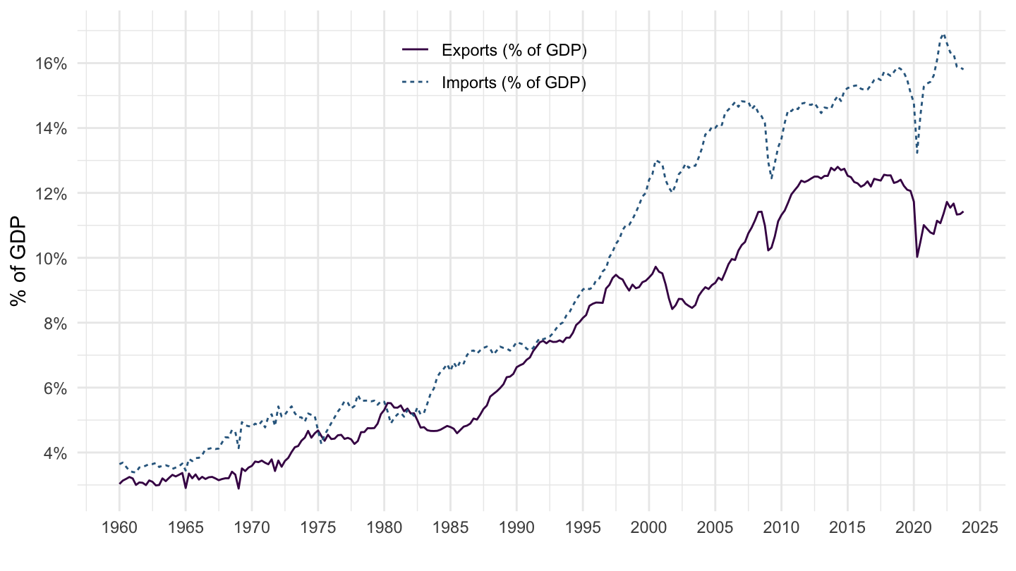
Figure 11.1: Exports and Imports, United States (percentage of GDP)

As we have just seen, the imbalance between exports and imports is itself driven by an imbalance between saving and investment. Figure 11.2 plots saving and investment as a percentage of GDP: depending on the period, booming investment is either financed locally, or through a current account deficit.

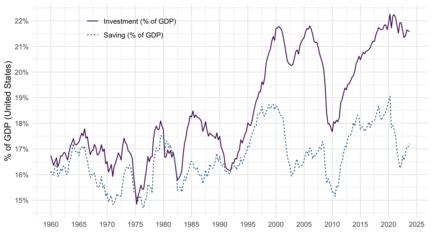
Figure 11.2: Saving and Investment, United States (percentage of GDP)

Figure 11.3 plots exports and imports in Germany as a percentage of GDP. Again, even more strikingly than in the U.S. case, both exports and imports are a rising share of GDP. However, this time, exports are usually much higher than imports.

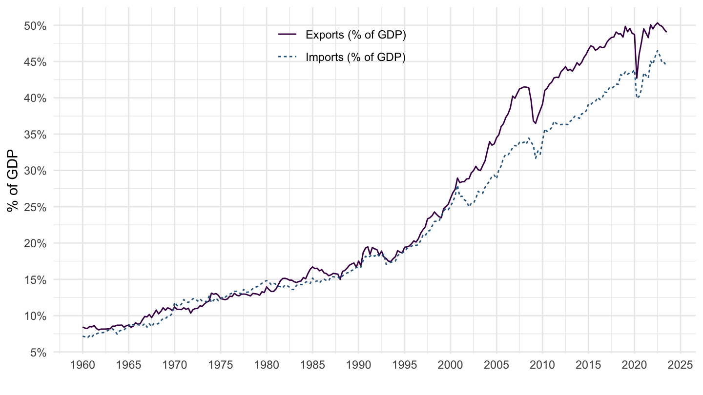
Figure 11.3: Exports and Imports, Germany (percentage of GDP)

The excess of exports over imports reflects an imbalance between saving and investment. Figure 11.4 plots saving and investment as a percentage of GDP. Since the end of the 90s, there has been a rise in saving in Germany, which has not translated into more investment, but on the contrary in more exports abroad.

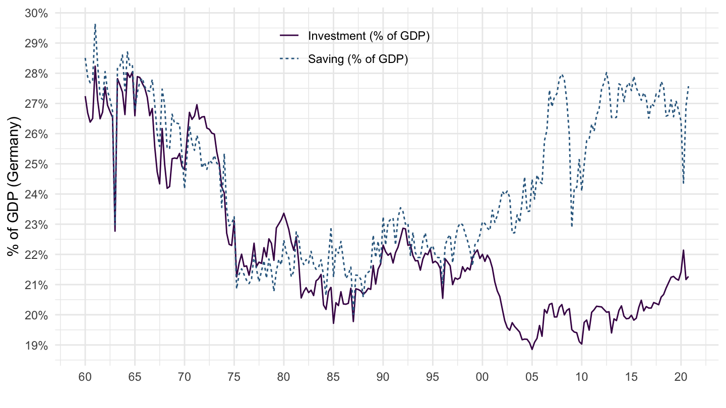
Figure 11.4: Saving and Investment, United States (percentage of GDP)

Table 11.1 shows that Russia, Ireland, the Netherlands, South Korea, and Switzerland are in a similar situation as Germany: they have an excess of exports over imports. In contrast, the United States have a large trade deficit, which is about twice as large as Germany’s trade surplus.

Table 11.1: Largest trades surpluses / deficits, in $ (Source: OECD)
Country	2000	2009	2018
Euro area (19 countries)	$84 Bn	$132 Bn	$754 Bn
Germany	$15 Bn	$106 Bn	$314 Bn
Russia	$218 Bn	$118 Bn	$308 Bn
Ireland	$14 Bn	$25 Bn	$137 Bn
Netherlands	$26 Bn	$51 Bn	$104 Bn
Korea	$12 Bn	$96 Bn	$93 Bn
Switzerland	$11 Bn	$0 Bn	$79 Bn
Italy	$22 Bn	$-19 Bn	$73 Bn
Spain	$-26 Bn	$-11 Bn	$60 Bn
Brazil	$-9 Bn	$10 Bn	$45 Bn
Poland	$-28 Bn	$-12 Bn	$38 Bn
Japan	$55 Bn	$-32 Bn	$37 Bn
Indonesia	$106 Bn	$29 Bn	$-14 Bn
Argentina		$37 Bn	$-29 Bn
Colombia		$-14 Bn	$-31 Bn
United Kingdom	$-23 Bn	$-33 Bn	$-34 Bn
Canada	$43 Bn	$-18 Bn	$-40 Bn
Mexico	$-11 Bn	$-37 Bn	$-45 Bn
Turkey	$-22 Bn	$11 Bn	$-124 Bn
India	$-62 Bn	$-172 Bn	$-226 Bn
G7	$-215 Bn	$-413 Bn	$-302 Bn
United States	$-352 Bn	$-396 Bn	$-629 Bn
NAFTA	$-320 Bn	$-451 Bn	$-714 Bn