10 Public Debt
Link to slides / Link to handouts
Is government debt a problem? Does government debt crowd out private capital accumulation? What is an optimal level of government debt? These are very important issues, and ones that are fiercely debated by macroeconomists, and policymakers around the world.
Until now, we have been talking about government spending and taxes as if the government could take on as much debt as it wants. But then, why doesn’t the government just engage in more tax cutting and more government spending, or both? We alluded to a first reason when we talked about the consequences of having \(1-c_1<b_1\), or the propensity to save be less than the propensity to invest. We argued then that we would never be in a Keynesian situation of deficient aggregate demand, so that multiplier effects would stop when facing constraints on supply. Similarly, if the government started to make public saving very negative (running a budget deficit), then it would similarly start facing constraints on what the economy can supply. For instance, if fiscal policy was too accommodative, and to the limit if \(G\) was set at too high a value, then supply constraints would start to bite: one example was given historically in the 1940s when the U.S. engaged in World War II. However, these levels of spending are clearly out of the question, and this is perhaps not what constrains the government from doing a little bit more spending, or a little bit more tax reductions.
To take a recent example, the Trump tax cuts that have just been enacted have reduced unemployment to historically low levels, and pushed GDP growth up to highs that have not been seen in a long time, as predicted by the Keynesian model. So what is the problem with these tax cuts? Why do many mainstream economists complain about them?
The reason is that these tax cuts have obviously raised U.S. public debt, and in fact they are mostly being criticized on these grounds. This makes sense: when government spending increases \(\Delta G>0\), this leads to a government deficit of equal magnitude: \(\Delta (T-G) = -\Delta G<0.\) Similarly, a tax cut \(\Delta T<0\) leads to increased deficits given by \(\Delta (T-G) = \Delta T<0\).28 One might worry that this debt will someday have to be repaid, and that the current generation is simply putting a burden on future generations. In this case, higher GDP today might only be thought of as leading to lower GDP in the future, when aggregate demand will be diminished.
During this lecture, we make three related points concerning government deficits and government debt:
We show first, without using any economic model, that simple accounting suggests that public debt is on a sustainable path whenever the real interest rate on public debt is lower than the rate of growth of GDP (\(r<g\)), a situation called “dynamic inefficiency” for reasons that will become clear later. (from problem set 4 you may already remember that the Golden Rule level of capital accumulation corresponded to \(r=g\)). I shall argue that real interest rates appear to be below the rate of growth of GDP, at least for now, so there does not seem to be cause for alarm - at least, until interest rates don’t rise more.
Second, I illustrate using an economic model that it is not true that public debt necessarily will need to be repaid eventually, so that government debt is not necessarily a burden on future generations - an argument which is often made in the public debate. In the overlapping generations model, and provided that capital accumulation is above the Golden Rule level (\(r<g\)), so that there is dynamic inefficiency, public debt is never repaid, as there are always new generations coming along, who buy government debt when they are young and sell it to the next generation when old. This is sustainable whenever \(r \leq g\), for reasons laid out in part one.
Third and last, we shall discuss the effects of larger government deficits on the economy, and constrast the Keynesian and Neoclassical views on this issue. In particular, Keynesian and Neoclassical economists have very different predictions for the impact of higher public deficits on investment spending. We discuss this and related issues surrounding the so-called Treasury View and Say’s law in the last section of this lecture.
Finally, we shall be looking at some data: some data on government debt, some data on interest rates. In particular we shall be discussing a common misconception: that the Greek’s debt crisis, or similarly Italy’s relatively high interest rates on government debt, show that the crowding out hypothesis is right, and that interest rates do rise when more government debt is undertaken.
10.1 Law of motion for Public Debt
In this lecture, we denote everything in terms of goods (that is, in real terms), to avoid thinking about the complicated issues surrounding inflation. We shall denote by \(G_t\) the government spending at period \(t\), and by \(T_t\) the taxes in period \(t\). Let us also denote by \((G_t-T_t)\) the government (primary) deficit in period \(t\), which is the excess of government expenditures over taxes levied by the government (thus, when \(G_t-T_t>0\), there is a deficit in the budget, so that the government must borrow). If the interest rate that the government pays is given by \(r_t\), then the law of motion of government debt is given by: \[B_{t}=(1+r_t)B_{t-1}+G_{t}-T_{t}.\]
The total government deficit, which is equal to the change in government debt \(\Delta B_{t}\), is equal to the sum of interest payments and the primary deficit \(G_{t}-T_{t}:\) \[\text{Deficit}_{t}=\Delta B_{t}=B_{t}-B_{t-1}=\underbrace{r_tB_{t-1}}_{\text{Interest Payments}}+\underbrace{G_{t}-T_{t}}_{\text{Primary Deficit}}\] From the above equation, the evolution of the debt to GDP ratio \(B_{t}/Y_{t}\): \[\frac{B_{t}}{Y_{t}}=(1+r_t)\frac{Y_{t-1}}{Y_{t}}\frac{B_{t-1}}{Y_{t-1}}+\frac{G_{t}-T_{t}}{Y_{t}}\] Let us denote the debt to GDP ratio by \(b_t\): \[b_t \equiv \frac{B_t}{Y_t}.\] Therefore: \[b_t = (1+r_t)\frac{Y_{t-1}}{Y_{t}}b_{t-1}+\frac{G_{t}-T_{t}}{Y_{t}}.\] Assuming that GDP grows at rate \(g_Y\), we have that: \[\frac{Y_t}{Y_{t-1}}=1+g_Y.\] Therefore: \[\boxed{b_t = \frac{1+r_t}{1+g_Y}b_{t-1}+\frac{G_{t}-T_{t}}{Y_{t}}}.\]
10.2 Condition for Sustainability of Public Debt
A thought experiment is useful to think about the sustainability of public debt in this environment. Imagine that all future primary surpluses were equal to zero after \(t=t_0\), that is: \[\text{for all }t\geq t_{0},\quad G_{t}=T_{t},\] and that real interest rates are constant after \(t \geq t_0\): \[r_t=r.\] We then have that: \[\text{for all }t\geq t_{0},\quad b_t = \frac{1+r}{1+g_Y}b_{t-1}.\]
Then the debt to GDP ratio would be given by: \[\boxed{\text{for all }t\geq t_{0},\quad b_t=\left(\frac{1+r}{1+g_Y}\right)^{t-t_{0}}b_{t_0}}\]
There are three possible cases:
- If \(r<g_Y\) - a situation called dynamic inefficiency29 - the debt to GDP ratio goes to 0. (Indeed, when \(a<1\), \(a^{t}\to 0\) when \(t \to +\infty\).) Therefore, the debt to GDP ratio goes to zero.
If \(r=g_Y\), the debt to GDP ratio stays constant. Then, the debt to GDP ratio stays constant.
If \(r>g_Y\), the debt to GDP ratio goes to infinity. Indeed, when \(a>1\), \(a^{t}\to+\infty\) when \(t \to +\infty\). Then, the debt to GDP ratio goes to infinity.
Is public debt sustainable in the U.S.? Which of these three cases is relevant for the U.S. economy? Is public debt sustainable in the U.S.? How do the real interest rate \(r\) and the growth rate of GDP \(g_Y\) compare? Up until now, I would argue that it’s fair to say that \(r<g_Y\).
The real interest rate \(r\) can be measured in two ways:
- Either using the nominal interest rate, and substracting an average expected (or realized) inflation rate in order to get to a real interest rate. Figure 10.1 shows that the nominal interest rate has averaged around 2 to 3% recently, while inflation has been from 1 to 2% on average. This implies a real interest rate which is around 1%, perhaps 2%.
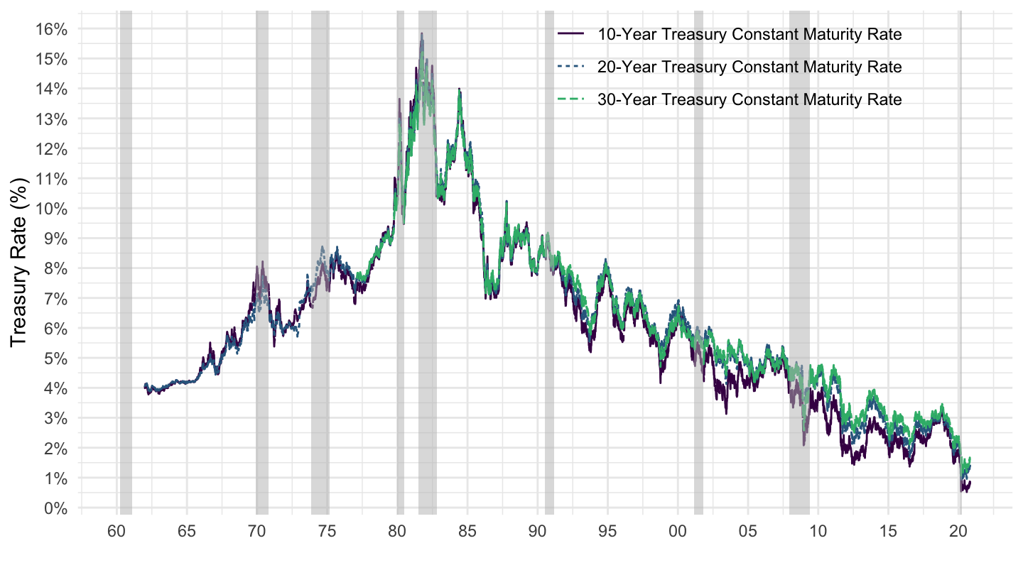
Figure 10.1: 10-Year Treasury Rate (Source: FRED).
- Or, one can measure the real interest rate by using the rate on Treasury Inflation Protected Securities (TIPS). Figure 10.2 from FRED (the Federal Reserve Economic Data) shows that the real interest rate has recently been around 1% per year.
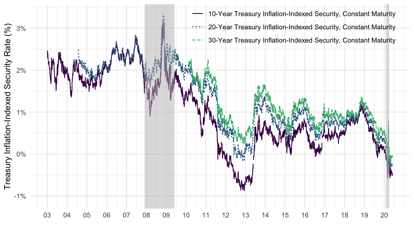
Figure 10.2: 10-Year Treasury Inflation Protected Securities Rate (Source: FRED).
On the other hand, real GDP growth seems to be hovering around \(g_Y \approx 2.5\%\). Real GDP per capita growth is variable, but it is usually estimated to be around 1.5%: \(g_{Y/L} \approx 1.5\%\). It varies over time, however: it was around 3.0% per year on average in the 1960s, 2.1% in the 1970s, 2.4% in the 1980s, 2.2% in the 1990s, 0.7% in the 2000s, and 0.9% from 2010 to 2017. On the other hand, the growth rate of population is around 1%: \(g_{L} \approx 1.5\%\). Therefore: \[ \begin{aligned} g_Y &= g_{Y/L} + g_L\\ &\approx 1.5\% + 1\% \\ g_Y &\approx 2.5\%. \end{aligned} \] Therefore, the ratio of government debt to GDP does not appear to be on an unsustainable path so far. Table ?? gives \(r-g\) across countries, as of November 2019. r-g is everywhere negative, not just in the United States.
| Country | i | pi | r = i-pi | g | r - g |
|---|---|---|---|---|---|
| Australia | 1.03% | 2.58% | -1.55% | 3.12% | -4.67% |
| Austria | -0.2% | 1.56% | -1.76% | 1.84% | -3.6% |
| Belgium | -0.16% | 1.55% | -1.71% | 1.85% | -3.56% |
| Canada | 1.45% | 1.89% | -0.44% | 2.39% | -2.83% |
| Czech Republic | 1.32% | 2.75% | -1.43% | 2.52% | -3.95% |
| Denmark | -0.43% | 1.78% | -2.21% | 1.59% | -3.79% |
| Finland | -0.21% | 1.63% | -1.84% | 2.18% | -4.02% |
| France | -0.16% | 1.25% | -1.41% | 1.61% | -3.02% |
| Germany | -0.47% | 1.05% | -1.52% | 1.42% | -2.94% |
| Greece | 1.34% | 2.17% | -0.83% | 0.8% | -1.63% |
| Hungary | 1.94% | 6.19% | -4.25% | 2.45% | -6.71% |
| Iceland | 0.84% | 4.33% | -3.49% | 3.53% | -7.01% |
| Ireland | 0% | 2.3% | -2.3% | 5.42% | -7.72% |
| Italy | 1% | 1.93% | -0.93% | 0.59% | -1.52% |
| Japan | -0.15% | -0.58% | 0.43% | 0.86% | -0.43% |
| Korea | 1.58% | 2.17% | -0.59% | 4.18% | -4.77% |
| Luxembourg | -0.39% | 2.38% | -2.77% | 3.43% | -6.2% |
| Mexico | 6.87% | 7.4% | -0.53% | 2.69% | -3.22% |
| Netherlands | -0.31% | 1.71% | -2.02% | 2% | -4.03% |
| New Zealand | 1.16% | 2.05% | -0.89% | 2.93% | -3.82% |
| Norway | 1.26% | 3.62% | -2.36% | 2.03% | -4.39% |
| Poland | 1.96% | 3.97% | -2.01% | 4% | -6.01% |
| Portugal | 0.19% | 2.26% | -2.07% | 1.34% | -3.41% |
| Slovak Republic | -0.2% | 2.78% | -2.98% | 3.8% | -6.78% |
| Spain | 0.2% | 2.04% | -1.84% | 2.13% | -3.97% |
| Sweden | -0.16% | 1.57% | -1.73% | 2.5% | -4.23% |
| Switzerland | -0.51% | 0.4% | -0.91% | 1.91% | -2.82% |
| United Kingdom | 0.64% | 1.92% | -1.28% | 2.09% | -3.38% |
| United States | 1.71% | 1.87% | -0.16% | 2.44% | -2.6% |
| Chile | 2.94% | 4.19% | -1.25% | 3.77% | -5.01% |
| Israel | 0.88% | 2.8% | -1.92% | 3.65% | -5.56% |
| Slovenia | -0.09% | 3.73% | -3.82% | 2.64% | -6.46% |
| South Africa | 8.93% | 6.69% | 2.24% | 2.66% | -0.43% |
| Latvia | 0% | 4.68% | -4.68% | 3.9% | -8.59% |
| Costa Rica | 10.2% | 8.32% | 1.88% | 3.97% | -2.1% |
| Lithuania | 0.31% | 3.58% | -3.27% | 4.09% | -7.36% |
A final way to see that U.S. debt is not (or not yet) on an unsustainable path is to note that the ratio of interest payments to GDP is not particularly high historically, which is shown on Figure 10.3. This implies that if the primary deficit was reduced to zero, the debt to GDP ratio would not be on an explosive trajectory.
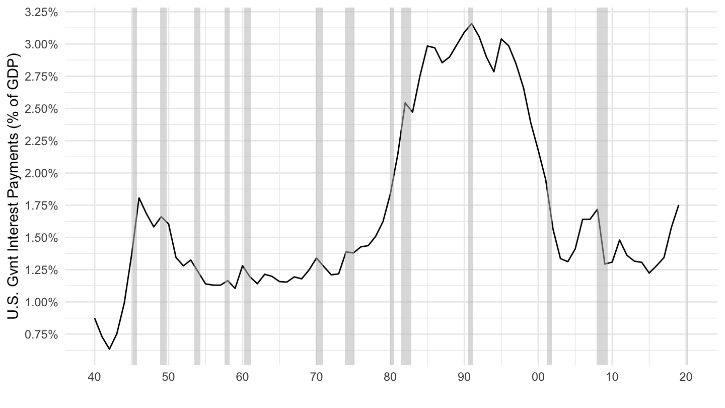
Figure 10.3: Interest Payments on Government Debt as % of GDP (Source: FRED).
10.3 Public Debt in the Overlapping Generations Model
In this section, I illustrate using the (neoclassical) overlapping-generations model that public debt does not necessarily need to be repaid eventually, so that government debt is not necessarily a burden on future generations - an argument which we nonetheless often hear in the public debate. However, one precondition for this is naturally that the debt to GDP has to be stable: we need that \(r^{*} \leq g_Y\). In the overlapping-generations model of lecture 4, we had \(g_Y = 0\), since there was no long-run growth. So we want \(r^{*} \leq 0\). In order to have a role for public debt, we will look at the model that we studied before.
Overlapping Generations Model. Let us look at a simplified version of the overlapping generations model we looked at in lecture 4. For this model, we shall assume that people only care about old age consumption, and that they work only when young, receiving wage \(w_{t}\). As we saw before, it does not really matter what the form of their utility function is with respect to old age consumption, because they will save everything anyway: \[U=u(c_{t+1}^{o}).\]
Denoting by \(r_t\) the (net) real interest rate, their intertemporal budget constraint is then given by: \[c_{t}^{y}+\frac{c_{t+1}^{o}}{1+r_t}=w_{t}.\] In this very simple environment, and because consumption in young age will always optimally be set to zero (\(c_{t}^{y}=0\)), this implies: \[c_{t+1}^{o}=(1+r_t)w_{t}.\] Similarly to the previous time, we assume that the labor force is fixed to unity (\(L_{t}=\bar{L}=1\)). The production function is Cobb-Douglas: \[Y_{t}=K_{t}^{\alpha}L_{t}^{1-\alpha}.\] Together with the previous assumption of constant labor \(L_{t}=1\), this implies that: \[Y_{t}=K_{t}^{\alpha}.\] From firms’ optimality conditions, the wage is just the marginal product of labor: \[w_{t}=\frac{\partial Y_{t}}{\partial L_{t}}=(1-\alpha)K_{t}^{\alpha}L_{t}^{-\alpha}=(1-\alpha)K_{t}^{\alpha}.\] Finally, for simplicity, we shall assume that the depreciation rate is equal to \(\delta=1=100\%\). In other words, capital fully depreciates each period - this is reasonable if you take one unit of time to represent one generation, or about 30 years - remember that the depreciation rate for one year was ranging from 5% to 10%. This implies that firms’ optimization on the amount of capital is the following equation: \[1+r_t=\frac{\partial Y_{t}}{\partial K_{t}}=\alpha K_{t}^{\alpha-1}.\]
Without Government Debt. Let us first remind ourselves what happens in the absence of government debt in this model. In the absence of a government, we get even simpler expressions than the previous time. With full depreciation (\(\delta=1\)), the law of motion for capital is given as: \[\Delta K_{t+1}=w_{t}- K_{t}.\] Since \(w_t\) is a fraction \(1-\alpha\) of output, this law of motion corresponds to the Solow growth model with \(s = 1-\alpha\). The law of motion for capital is: \[K_{t+1}=(1-\alpha) K_{t}^{\alpha}.\] This is a difference equation for sequence \(K_{t}\) which converges to a steady state value for the capital stock \(K^{*}\) such that: \[ \begin{aligned} & K^{*} = (1-\alpha)(K^*)^{\alpha}\\ & \quad \Rightarrow \quad K^{*}=(1-\alpha)^{\frac{1}{1-\alpha}}. \end{aligned} \] The steady state value for the interest rate \(r^{*}\) is then such that: \[ \begin{aligned} 1+ r^{*}&=\alpha(K^{*})^{\alpha-1}\\ &= \alpha \left[(1-\alpha)^{\frac{1}{1-\alpha}}\right]^{\alpha-1}\\ 1+r^{*} &=\frac{\alpha}{1-\alpha} \end{aligned} \] Therefore, the steady-state value of the interest rate \(r^{*}\) is: \[r^{*} = \frac{2\alpha-1}{1-\alpha}\] which is negative for \(\alpha < 1/2\). The steady state value for output \(Y^{*}\) is then: \[ \begin{aligned} Y^{*}&=\left(K^{*}\right)^{\alpha}\\ Y^{*}&=(1-\alpha)^{\frac{\alpha}{1-\alpha}}. \end{aligned} \] The value for the wage \(w^{*}\) is: \[ \begin{aligned} w^{*}&=(1-\alpha)\left(K^{*}\right)^{\alpha}\\ &=(1-\alpha)(1-\alpha)^{\frac{\alpha}{1-\alpha}}\\ w^{*} &= \left(1-\alpha\right)^{\frac{1}{1-\alpha}} \end{aligned} \] Steady-state consumption of the old \((c^{o})^{*}\) is thus given by: \[ \begin{aligned} (c^{o})^{*}&=(1+r^*)w^{*}\\ &=\left(1+ \frac{2\alpha-1}{1-\alpha}\right)\left(1-\alpha\right)^{\frac{1}{1-\alpha}}\\ &=\frac{\alpha}{1-\alpha}\left(1-\alpha\right)^{\frac{1}{1-\alpha}}\\ (c^{o})^{*}&= \alpha\left(1-\alpha\right)^{\frac{\alpha}{1-\alpha}} \end{aligned} \]
Numerical Application. For concreteness, we can look at a case where \(\alpha = 1/3\): \[ \begin{aligned} K^{*}&=(1-\alpha)^{\frac{1}{1-\alpha}}=\left(\frac{2}{3}\right)^{3/2}=\frac{2\sqrt{2}}{3\sqrt{3}}\\ r^{*}&=\frac{2\alpha-1}{1-\alpha}=\frac{-1/3}{2/3}=-\frac{1}{2}=-50\%\\ Y^{*}&=(1-\alpha)^{\frac{\alpha}{1-\alpha}} = \left(\frac{2}{3}\right)^{1/2}=\frac{\sqrt{2}}{\sqrt{3}}\\ w^{*}&=\left(1-\alpha\right)^{\frac{1}{1-\alpha}} =\frac{2\sqrt{2}}{3\sqrt{3}}\\ (c^{o})^{*}&=\alpha\left(1-\alpha\right)^{\frac{\alpha}{1-\alpha}}=\frac{1}{3} \left(\frac{2}{3}\right)^{1/2}=\frac{\sqrt{2}}{3\sqrt{3}} \end{aligned} \]
With Government Debt. Because \(r^{*}<0\) we have that the quantity of capital is higher than the Golden Rule level of the capital stock, which is such that \(r^{*}_g=0\). Why, again, is the Golden rule interest rate equal to 0 when there is no growth ? One quick way to understand it is to write that in the steady-state, the consumption of the old \((c^{o})^{*}\) is supposed to be maximized (since the old are the only ones consuming). However, we also know that in the steady-state, total production \(F(K^{*}, 1) = (K^{*})^{\alpha}\) is used for two things: consuming (for the old) and repairing the capital stock (saving equals investment equals depreciation, as in the Solow growth model), so that: \[(c^{o})^{*} + K^{*} = (K^{*})^{\alpha} \quad \Rightarrow \quad (c^{o})^{*} = (K^{*})^{\alpha} -K^{*} \] Therefore, the Golden rule capital stock \(K^{*}_g\), which maximizes \((c^{o})^{*}\) solves: \[\max_{K^{*}}\quad (K^{*})^{\alpha}-K^{*},\] which implies that: \[\alpha (K^{*}_g)^{\alpha-1}=1.\] Moreover, we know that the marginal product of capital \(\partial F(K^{*}, 1)/\partial K^{*} = \alpha (K^{*}_g)^{\alpha-1}\) is also equal to \(r^{*}_g+1\), the gross return, from the firms’ problem, which gives the following optimality condition: \[\alpha (K^{*}_g)^{\alpha-1}=r^{*}_g+1.\] Using these two last equalities allows to conclude that in this situation with no growth, the Golden rule interest rate is equal to zero since \(r^{*}_g+1 = \alpha (K^{*}_g)^{\alpha-1} =1\): \[r^{*}_g=0.\] However, we saw in the previous section that the equilibrium interest rate \(r^{*}\) was negative, equal to -50%. Therefore, the capital stock is too high here.
One way to solve this problem would be to force everyone to save less, in order to decrease private saving; however this might be thought of as a little bit too intrusive. Another way to solve this problem is to use public debt (decrease public saving, to reduce total saving) in order to solve this problem of excess saving and excess investment.
In order to better understand which level of public debt is warranted, we look at the level of capital such that \(r^{*}_g=0\) - which again, is the golden rule interest rate, since the rate of growth of output is \(g_Y=0\). Thus, the corresponding Golden Rule level of the capital stock \(K^{*}_g\) is such that: \[r^{*}_g+1=\alpha (K^{*}_g)^{\alpha-1} \quad \Rightarrow_{r^{*}_g=0} \quad 1=\alpha (K^{*}_g)^{\alpha-1}\] Therefore: \[ \begin{aligned} K^{*}_g=\alpha^{\frac{1}{1-\alpha}}. \end{aligned} \] The Golden rule steady-state value for output \(Y^{*}_g\) is: \[ \begin{aligned} Y^{*}_g&=\left(K^{*}_g\right)^{\alpha}\\ Y^{*}_g&=\alpha^{\frac{\alpha}{1-\alpha}}. \end{aligned} \] The value for the steady-state wage \(w^{*}_g\) is then: \[ \begin{aligned} w^{*}_g&=(1-\alpha)\left(K^{*}\right)^{\alpha}\\ w^{*}_g&=(1-\alpha) \alpha^{\frac{\alpha}{1-\alpha}} \end{aligned} \] Steady-state consumption of the old \((c^{o})^{*}_g\) is thus given by: \[ \begin{aligned} (c^{o})^{*}_g&=(1+r^*)w^{*}_g\\ (c^{o})^{*}_g&=(1-\alpha) \alpha^{\frac{\alpha}{1-\alpha}} \end{aligned} \]
The question is how to we achieve this quantity of capital \(K^{*}_g\)? The answer is that some public debt needs to be taken on by the government. Again, saving is equal to the wage \(w^{*}_g\), and to the purchase of total assets, which includes both public debt whose quantity is given by \(B^{*}_g\), and the capital stock whose quantity is \(K^{*}_g\). Therefore, we may compute the level of the public debt which allows to reach this Golden-Rule level of capital accumulation: \[B^{*}_g+K^{*}_g=w^{*}_g\quad\Rightarrow\quad B^{*}_g=w^{*}_g-K^{*}_g.\] Substituting: \[ \begin{aligned} B^{*}_g&=w^{*}_g-K^{*}_g\\ &=(1-\alpha) \alpha^{\frac{\alpha}{1-\alpha}}-\alpha^{\frac{1}{1-\alpha}}\\ B^{*}_g&=\alpha^{\frac{\alpha}{1-\alpha}}\left(1-2\alpha\right). \end{aligned} \] Note that this level of public debt is strictly positive when \(\alpha <1/2\). This is intuitive: whenever we have dynamic inefficiency, the government should take on public debt.
Note also that the return on total saving \(w_g^{*}\) can be broken down between the return on public debt, and the return on private capital, so that: \[(c^{o})^{*}_g=\underbrace{(1+r^*_g)K^{*}_g}_{\text{Return on private capital}} + \underbrace{(1+r^*_g)B^{*}_g}_{\text{Return on public debt}}\]
Numerical Application. With \(\alpha = 1/3\): \[ \begin{aligned} K^{*}_g&=\alpha^{\frac{1}{1-\alpha}}=\left(\frac{1}{3}\right)^{3/2} = \frac{1}{3\sqrt{3}}\\ r_g^{*}&=0\\ Y_g^{*}&=\alpha^{\frac{\alpha}{1-\alpha}} = \left(\frac{1}{3}\right)^{1/2}=\frac{1}{\sqrt{3}}\\ w^{*}_g&=(1-\alpha) \alpha^{\frac{\alpha}{1-\alpha}}= \frac{2}{3}\sqrt{\frac{1}{3}} = \frac{2}{3\sqrt{3}}\\ (c^{o})^{*}_g&=(1+r^*_g)w^{*}_g=w^{*}_g = \frac{2}{3\sqrt{3}} \end{aligned} \] Note that the steady-state consumption of the old \((c^{o})^{*}_g\) is greater than the level of consumption achieved by the old without government debt since \(2>\sqrt{2}\). But what is amazing is that the level of capital in this case is actually lower than the level of capital in the previous section. The government can force the economy into this level of capital accumulation by taking on debt.
The level of debt \(B^{*}_g\) that corresponds to that level of capital accumulation is given by: \[ \begin{aligned} B^{*}_g&=w^{*}_g-K^{*}_g\\ &=\frac{2}{3\sqrt{3}}-\frac{1}{3\sqrt{3}}\\ B^{*}_g&=\frac{1}{3\sqrt{3}}. \end{aligned} \]
The government can reach that level of debt by giving a transfer to the first generation of old, who will then consume in the first period \(t=0\) an amount equal to: \[c_{0}^{o}=\frac{\sqrt{2}}{3\sqrt{3}}+\frac{1}{3\sqrt{3}}=\frac{1+\sqrt{2}}{3\sqrt{3}}.\] All future generations thus consume more. With a lot of capital, there is such a thing as a free lunch! Public debt is a Ponzi scheme, but a beneficial one. Public debt allows to increase consumption for everyone, and it can be rolled over every period (note that the debt to GDP ratio stays constant, as GDP growth is zero in the long run, just as the long run interest rate is zero). This is true more generally even in the neoclassical model, provided that there is dynamic inefficiency (\(r^*<g_Y\)) to begin with.
10.4 Pay-As-You-Go Systems, and “Rational Bubbles”
The overlapping generations model also allows us to think about pay-as-you-go systems, as well as about something called “rational bubbles.” I now turn to these two topics.
Pay-As-You-Go (PAYG). A Pay-As-You-Go (PAYG) system is an alternative arrangement, economically equivalent to explicit public debt, but which apparently takes a very different form. Assume that instead of taking out public debt, the government taxes the young generation in the first period, in order to transfer money to the old generation. Denote this amount of taxation by \(T^{y*}_g>0\). Again, we have: \[T^{y*}_g+K^{*}_g=w^{*}_g\quad\Rightarrow\quad T^{y*}_g=w^{*}_g-K^{*}_g.\]
When old, people receive their returns to capital, and a transfer by the government equal to what they had put into the system \(T_g^{o*}>0\), so that their return on social security is the same as what they would have gotten on the private market (the net return is equal to \(0\)): \[T_g^{o*}=T_g^{y*}.\]
As The Economist magazine explains in a briefing on overlapping generations models:30
This intergenerational logic lies behind the “pay-as-you-go” (PAYG) pensions common in many countries. People contribute to the scheme during their working lives, and receive a payout in retirement. Many people fondly imagine that their contributions are saved or invested on their behalf, until they reach pensionable age. But that is not the case. The contributions of today’s workers pay the pensions of today’s retirees. The money is transferred between generations, not across time.
Therefore, a pay-as-you-go system is exactly equivalent to public debt. It is sometimes referred to as implicit public debt. (although this is usually done to criticize it) During sections, we shall discuss this issue around a debate between Paul Krugman and Robert Barro, surrounding the issues of social security.
“Rational Bubbles.” When we looked at some data on capital and investment, we saw that the market value of capital is actually much greater than the book value of the capital stock. We also know that financial markets are subject to booms and busts episodes, which are very hard to reconcile with fundamentals (dividends, and interest rates). The overlapping-generations model can give an explanation for these puzzling phenomena. In an environment with low interest rates (dynamic inefficiency), assets can be bought at a price in excess of their book value, including a “bubble” component. This “bubble” component can grow at the rate of interest, when interest rates are relatively low, and overvaluation is justified by the fact that future generations will buy the overvalued asset as well. The Economist magazine explains it as follows:31
A third, more anarchic way to transfer resources from young to old is a speculative bubble. In a bubble, people pay over the odds for an asset, such as a house, in the belief that subsequent investors will pay a higher price still. The overpayment amounts to a contribution to a Ponzi scheme, redeemed not by the earnings of the underlying asset, but by overpayments from later investors. If each generation is collectively richer than the last, then the as- set’s price can keep rising even if each buy- er sinks only the same percentage of their (rising) income into it.
These bubbles are called “rational” because the force driving it is the excess of saving (low interest rates). When interest rates are low, buying a Ponzi scheme can lead to higher returns than buying a “real investment” instead (that is, book capital). As a consequence, the excess of saving can also explain why it is hard to make sense of high valuations on the real estate, or on the stock market; and why the market value of capital is so much greater than the book value of capital.
10.5 Treasury View: The Effects of Deficit Spending on Investment.
The most controversial and also most important questions in macroeconomics revolve around the issue of the so-called Treasury View, and Say’s law. These are probably the most difficult, controversial, but also the most important questions for macroeconomics. We start here with the Treasury View.
The Treasury View asserts that more government spending, either in the form of government purchases or of tax reductions, and therefore lower saving, necessarily leads to crowd out (reduce) an equal amount of investment spending. Conversely more saving, either by the government or by households, leads to more investment. The logic of this argument is rather straightforward: if there exists a finite amount of resources in the economy - in other words, output is supply-determined - then whatever is being saved goes to increase investment. Output is simply the sum of consumption, investment, and government spending, so that “necessarily” increasing government spending leads to crowd out either of every component: \[ \begin{aligned} &Y = C+I+G\\ \quad & \Rightarrow \quad \left(Y- C-T\right)=I+\left(G-T\right) \\ \quad & \Rightarrow \quad \left(Y- C-T\right) + \left(T-G\right)=I \end{aligned} \] Therefore investment \(I\) equals total saving, private saving \(S=Y-C-T\) plus public saving \(T-G\): \[\boxed{I = \underbrace{\left(Y-C-T\right)}_{\text{Private Saving}} + \underbrace{(T-G)}_{\text{Public Saving}}}\] The reason why this view is called the Treasury View is that it was advanced in the 1930s, during the Great Depression, by the staff of the British Chancellor of the Exchequer, Winston Churchill. When defending his 1929 budget, Winston Churchill explained:
The orthodox Treasury view… is that when the Government borrows in the money market it becomes a new competitor with industry and engrosses to itself resources which would otherwise have been employed by private enterprise, and in the process raises the rent of money to all who have need of it.
What we have seen so far leads us to take a very constrasted perspective on the Treasury View:
In the Keynesian model, investment is not crowded out by public debt - in the simplest model of the goods market, investment is in fact fixed. In the accelerator model, \(I=b_0 + b_1 Y\) so that investment depends only on sales, not on saving. According to this model, what the Treasury View misses is that output is not determined by supply, but it is instead determined by demand. Therefore, one cannot reason as if GDP was fixed: GDP is precisely what adjusts when saving is reduced, to maintain the equality between investment and total saving.
In the neoclassical model in contrast, investment is determined by total saving, and it moves flexibly in response to saving. According to this view, investment is indeed crowded out by public deficits. Note however that this does not mean that in the neoclassical model, government deficits are always bad. As we just saw, public deficits may be a good thing if the economy has too much capital to begin with.
This issue of the Treasury view was discussed a lot during the U.S. 2008 financial crisis, when policymakers were turning to economists for advice on the appropriate policy response. You can see some discussion of this issue in “Required Readings”. While Chicago economists were articulating the Treasury view in various different flavors, Keynesian economists were rejecting this notion very strongly - most notably Paul Krugman. Of course, whether the Treasury View is correct or not is ultimately an empirical question. We will present some empirical evidence on this issue during lecture 13.
10.6 Say’s law: supply creates its own demand.
Say’s law, named after Jean-Baptiste Say (1767 - 1832), has been summarized by J.M. Keynes as a statement that “supply creates its own demand”. Jean-Baptiste Say’s reasoning was straightforward:
It is worthwhile to remark that a product is no sooner created than it, from that instant, affords a market for other products to the full extent of its own value. When the producer has put the finishing hand to his product, he is most anxious to sell it immediately, lest its value should diminish in his hands. Nor is he less anxious to dispose of the money he may get for it; for the value of money is also perishable. But the only way of getting rid of money is in the purchase of some product or other. Thus the mere circumstance of creation of one product immediately opens a vent for other products.
Thus, in Jean-Baptiste Say’s opinion, supply creates its own demand, and there can never be any aggregate demand shortages. In an article on Say’s law, The Economist magazine writes:32
In Say’s time, as nowadays, the world economy combined strong technological progress with fitful demand, spurts of innovation with bouts of austerity. (…) On the other hand, global demand was damaged by failed ventures in South America and debilitated by the eventual downfall of Napoleon. In Britain government spending was cut by 40% after the Battle of Waterloo in 1815. Some 300,000 discharged soldiers and sailors were forced to seek alternative employment. The result was a tide of overcapacity, what Say’s contemporaries called a “general glut”. Britain was accused of inundating foreign markets, from Italy to Brazil, much as China is blamed for dumping products today. In 1818 a visitor to America found “not a city, nor a town, in which the quantity of goods offered for sale is not infinitely greater than the means of the buyers”. It was this “general overstock of all the markets of the universe” that came to preoccupy Say and his critics. In trying to explain it, Say at first denied that a “general” glut could exist. Some goods can be oversupplied, he conceded. But goods in general cannot. His reasoning became known as Say’s law: “it is production which opens a demand for products”, or, in a later, snappier formulation: supply creates its own demand.
Of course, one critical assumption underlying Say’s law is that working or accumulating wealth never are an end in themselves:
According to the logic of Say and his allies, people would not bother to produce anything unless they intended to do something with the proceeds. Why suffer the inconvenience of providing $100-worth of labour, unless something of equal value was sought in return? Even if people chose to save not con- sume the proceeds, Say was sure this saving would translate faithfully into investment in new capital, like his own cot- ton factory. And that kind of investment, Say knew all too well, was a voracious source of demand for men and materials. But what if the sought-after thing was $100 itself? What if people produced goods to obtain money, not merely as a transactional device to be swiftly exchanged for other things, but as a store of value, to be held indefinitely? A widespread propensity to hoard money posed a problem for Say’s vision. It interrupted the exchange of goods for goods on which his theory relied.
This can actually be argued with. For example, in a New York Times article, Alex Williams asks:33
“For most people, enough is enough,” said Robert Frank, the wealth editor for CNBC and the author of the 2007 book “Richistan: A Journey Through the American Wealth Boom and the Lives of the New Rich,” who has interviewed many plutocrats. “But there is another group of people, no matter what they have, they have to keep going. I call them ‘scorekeepers.’ They’re truly driven by competitive zeal.” Take Larry Ellison, the billionaire co-founder of Oracle. Mr. Ellison always felt competitive with Bill Gates and Paul Allen of Microsoft, Mr. Frank said. “So when Paul Allen built his 400-foot boat, Larry Ellison waited until it was done and built a 450-foot boat. Larry Ellison would never be happy until he was No. 1.”
Therefore, work is not necessarily done for the purpose of more consumption, but rather in order to amass large quantities of wealth. The rise in wealth inequality and of the “working rich” could therefore be one reason for the break of Say’s law.
Once again, we may contrast two quite different perspectives on the Say’s law, in the theoretical models we have previously described:
In the Keynesian model, supply does not create its own demand, as some resources (labor or capital) are idle. This allows government spending or tax cuts to have an effect on GDP, by utilizing some of these resources. The reason is that in this model, the desire to save does not necessarily translate into more investment, since investment is fixed or given by the overall level of GDP, which is depressed by more saving. Assuming that the propensity to save is larger than the propensity to invest \(1-c_1>b_1\), then we have a paradox of thrift: instead of increasing investment, a higher desire to save actually reduces output, which ends up depressing saving. Supply does not create its own demand, because one unit saved does not necessarily lead to more investment.
In the neoclassical model, investment is determined by total saving, and it moves flexibly in response to saving. According to this view, there can indeed never be a general glut: consumption increases aggregate demand, but saving increases it too, by stimulating more investment. At the same time, there might be “too much capital”, when the capital stock is higher than the Golden rule level, but this is not a “general glut”. Thus, supply can be thought of as indeed “creating its own demand”, even though at some point investment runs so much into diminishing returns that it’s better to issue government debt instead.
How you stand on those two issues - the Treasury View and Say’s law - determines whether you are more in line with the neoclassical or the Keynesian model. As we have seen however, Keynesians and neoclassicals agree on one thing: consumption is the sole purpose of all production, and there exists such a thing as “too much capital”, when \(r^{*}<g_Y\).
10.7 Data on the Quantities of Government Debt
We first look at some data on the quantity of government debt in different countries, over long periods of time. As shown on Figure 10.5, the level of government debt is currently around 100% of GDP in the U.S.. This sounds like a very big number (although one that does not make much sense, as it is comparing a stock of government debt to a flow of value added), but is it really? Let’s first look at the level of government debt in different countries. Table 10.2 shows countries with a public debt higher than 90% of GDP in 2015. Table 10.3 shows countries with a public debt ratio lower than 30% of GDP in 2015. Figure 10.4 plots debt to GDP ratios around the world, in 2015.
| Country | Public Debt (2015) |
|---|---|
| Japan | 248 % |
| Greece | 177 % |
| Lebanon | 138 % |
| Italy | 133 % |
| Portugal | 129 % |
| Azores | 129 % |
| Madeira Islands | 129 % |
| Eritrea | 127 % |
| Jamaica | 122 % |
| Cape Verde | 121 % |
| Cyprus | 109 % |
| Belgium | 106 % |
| Barbados | 105 % |
| USA | 105 % |
| Singapore | 105 % |
| Barbuda | 104 % |
| Antigua | 104 % |
| Spain | 99 % |
| Canary Islands | 99 % |
| France | 96 % |
| Clipperton Island | 96 % |
| Bhutan | 95 % |
| Jordan | 93 % |
| Gambia | 92 % |
| Canada | 91 % |
| Grenada | 91 % |
| Mauritania | 91 % |
| Country | Public Debt (2015) |
|---|---|
| San Marino | 20 % |
| Democratic Republic of the Congo | 19 % |
| United Arab Emirates | 18 % |
| Chile | 18 % |
| Swaziland | 17 % |
| Botswana | 17 % |
| Russia | 16 % |
| Iran | 16 % |
| Oman | 15 % |
| Equatorial Guinea | 14 % |
| Nigeria | 12 % |
| Kuwait | 11 % |
| Uzbekistan | 11 % |
| Solomon Islands | 10 % |
| Estonia | 10 % |
| Algeria | 9 % |
| Afghanistan | 6 % |
| Saudi Arabia | 5 % |
| Brunei | 3 % |
| China:Hong Kong | 0 % |
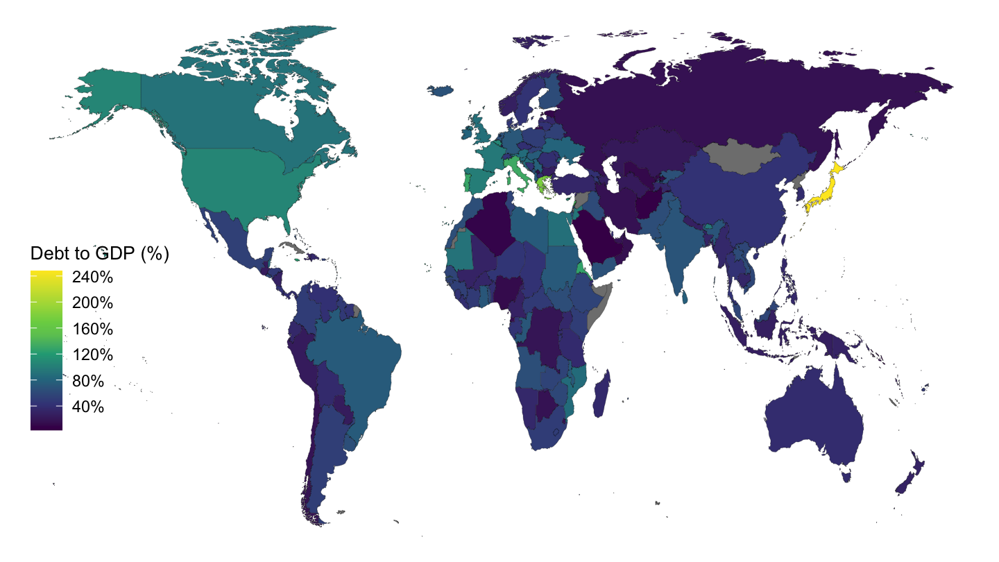
Figure 10.4: Debt to GDP (% of GDP), 2015.
Figure 10.5 shows that U.S. government debt is currently particularly high when compared to post World War 2 standards, while at the same time not exceptionally high compared to other periods, or even other countries. Most of the large rises in debt correspond to wars:
- U.S. debt, in the beginning of the 19th century, was recovering from the Revolutionary War (1775–1783).
- During the American Civil War (1861-1865), U.S. government debt also increased substantially, by about 40% of GDP.
- During World War I, U.S. government debt increased by about 20% of GDP.
- During World War II, U.S. government debt increased by about 50% of GDP.
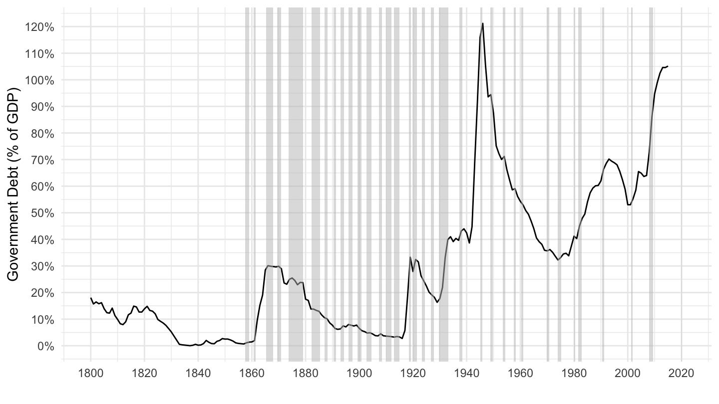
Figure 10.5: U.S. Government Debt (Source: IMF).
Another, even more striking example, is that of Japan: Figure 10.6 shows that Japan currently has much higher levels of government debt.
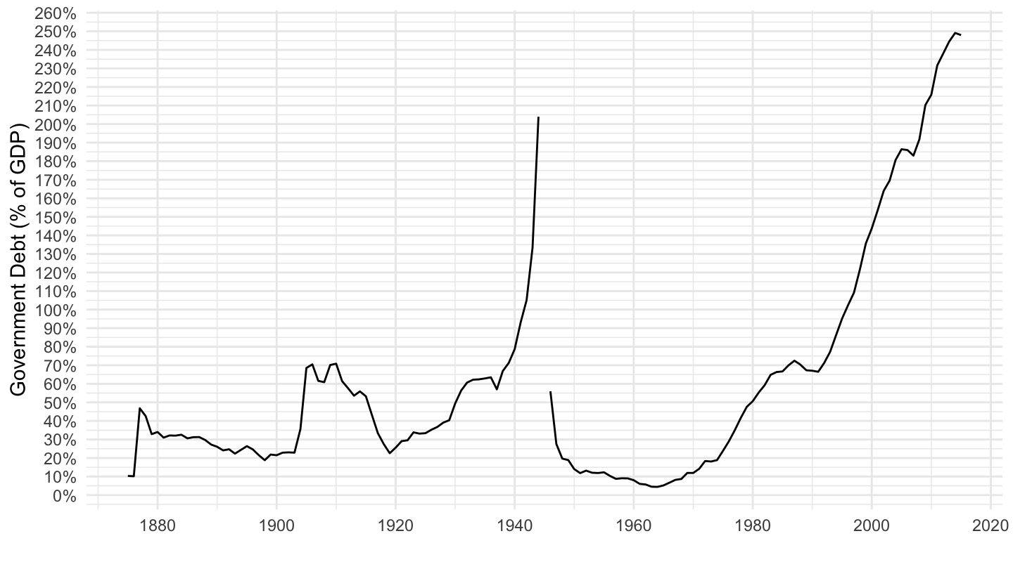
Figure 10.6: Japan’s Government Debt (Source: IMF).
Similarly, the U.K. was able to repay its debt contracted during the War against Napoleon during the whole nineteenth century, from a level of 260% of GDP, as shown on Figure 10.7.
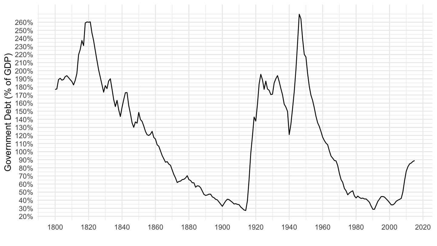
Figure 10.7: U.K. Government Debt (Source: IMF).
France also reached a level of government debt higher than 250% of GDP after World War II, as shown on Figure 10.8.
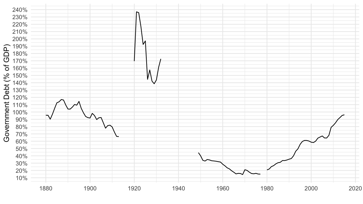
Figure 10.8: France’s Government Debt. Source: Global Financial Data.
It was able to reduce its level of government debt substantially after World Way II through inflation, as shown on Figures ?? which compares France, Germany and the United Kingdom.
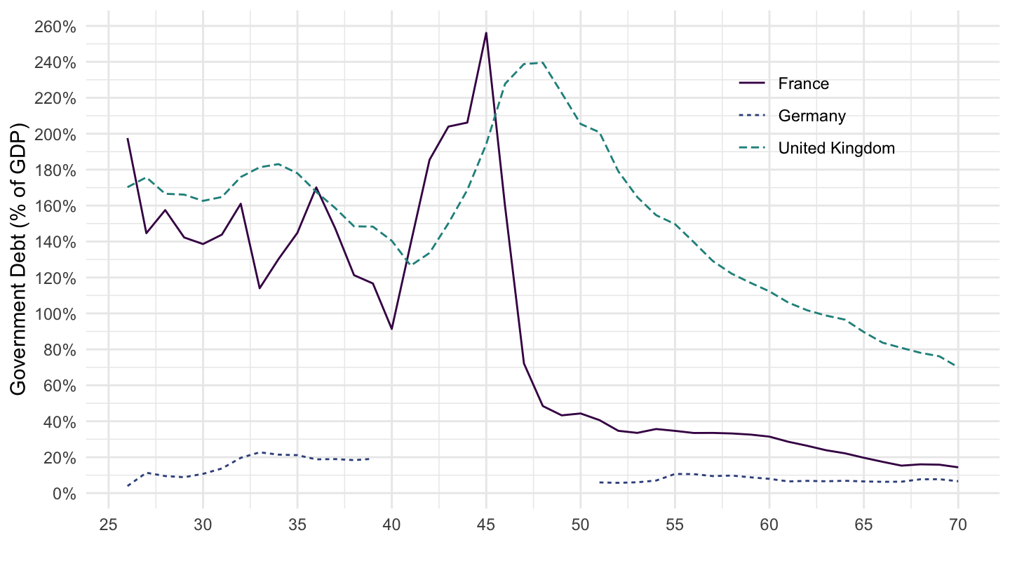
Figure 10.9: France, Germany, U.K. Government Debt. (% of GDP)
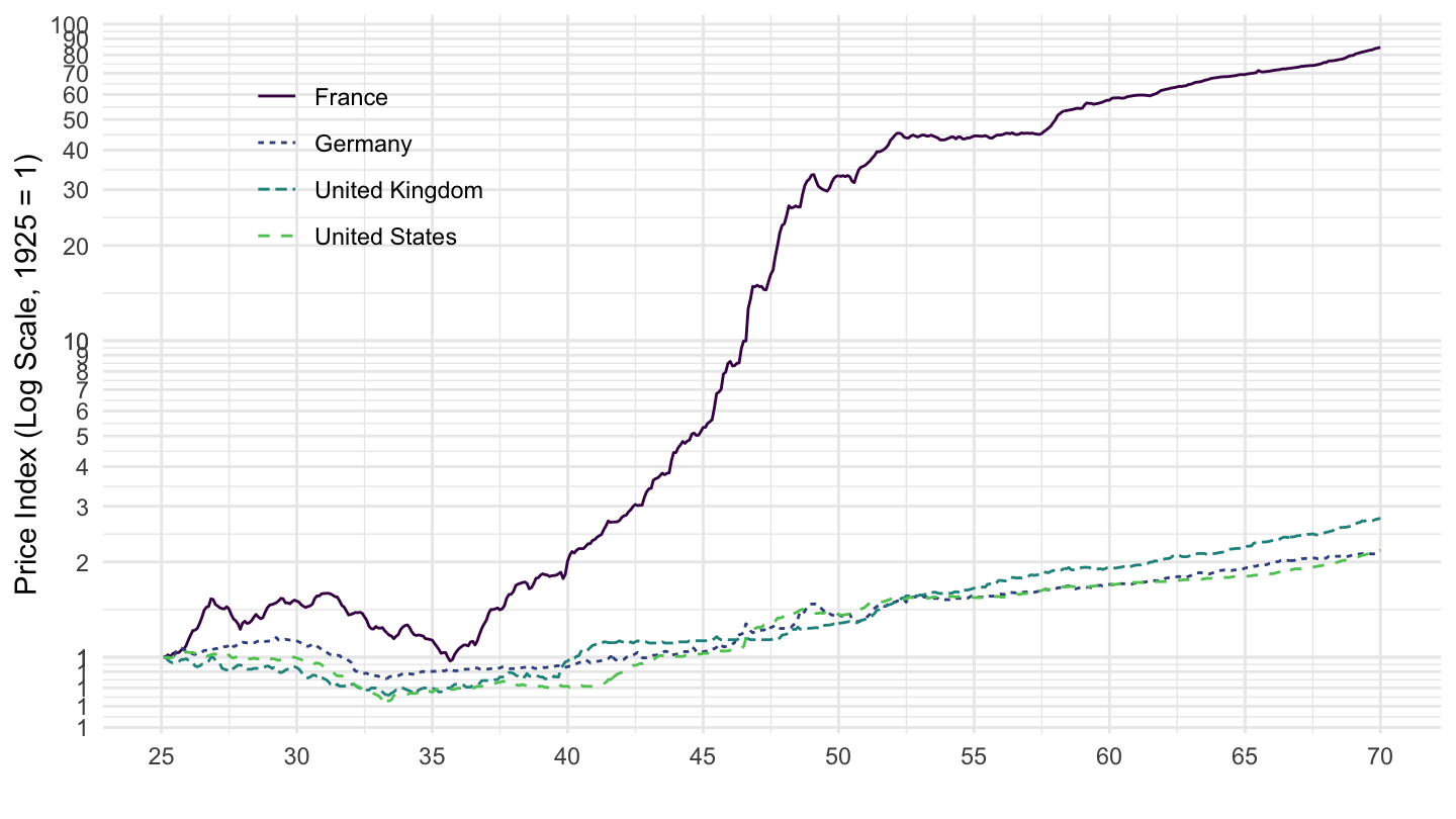
Figure 10.10: France, Germany, United Kingdom CPI (1925-1970).
In contrast, Germany has a much lower amount of government debt, one that is even declining, as can be seen on Figure 10.11.
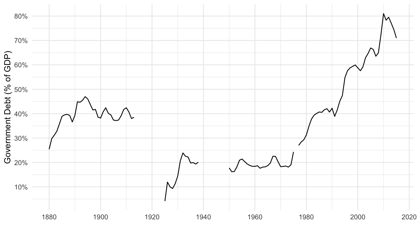
Figure 10.11: Germany’s Government Debt (Source: IMF).
10.8 Data on Primary Deficits
Table 10.4 shows average primary deficit around the world, according to Fiscal Monitor of the IMF. Figure 10.12 shows this data on a world map.
| Country | Primary Surplus (1995-2019) |
|---|---|
| Italy | 2.56 % |
| Belgium | 2.5 % |
| Algeria | 2.49 % |
| Brazil | 2.38 % |
| Russian Federation | 2.18 % |
| Philippines | 2.04 % |
| Korea, Republic of | 1.63 % |
| Turkey | 1.46 % |
| Canada | 1.4 % |
| Iceland | 1.33 % |
| Denmark | 1.28 % |
| Luxembourg | 1.28 % |
| Uruguay | 1.06 % |
| Greece | 1.03 % |
| Peru | 0.91 % |
| New Zealand | 0.82 % |
| South Africa | 0.8 % |
| Colombia | 0.78 % |
| Finland | 0.75 % |
| Thailand | 0.62 % |
| Switzerland | 0.52 % |
| Israel | 0.5 % |
| Germany | 0.48 % |
| Malta | 0.42 % |
| Netherlands | 0.38 % |
| Belarus | 0.31 % |
| Estonia | 0.23 % |
| Indonesia | 0.23 % |
| Ireland | 0.12 % |
| Cyprus | 0.11 % |
| Mexico | 0.07 % |
| Sweden | 0.01 % |
| Country | Primary Surplus (1995-2019) |
|---|---|
| Ecuador | -0.01 % |
| Slovenia | -0.05 % |
| Austria | -0.13 % |
| Argentina | -0.18 % |
| Chile | -0.18 % |
| Australia | -0.25 % |
| Ukraine | -0.62 % |
| Portugal | -0.63 % |
| NA | -0.7 % |
| Hungary | -0.79 % |
| France | -0.95 % |
| China | -0.95 % |
| Latvia | -1.15 % |
| Dominican Republic | -1.19 % |
| Spain | -1.21 % |
| Malaysia | -1.25 % |
| Croatia | -1.29 % |
| Morocco | -1.41 % |
| Poland | -1.44 % |
| United Kingdom | -1.6 % |
| Ghana | -1.75 % |
| Lithuania | -1.9 % |
| Kenya | -2.2 % |
| Romania | -2.35 % |
| Czech Republic | -2.42 % |
| Hong Kong, China | -2.56 % |
| Kyrgyzstan | -2.83 % |
| Slovakia | -2.91 % |
| United States | -2.96 % |
| Egypt | -3.59 % |
| India | -3.62 % |
| Japan | -4.67 % |
| Angola | -6.74 % |
| Norway | -6.93 % |
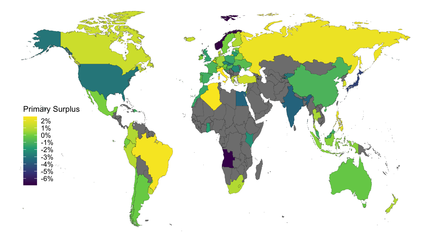
Figure 10.12: Average Primary Surpluses, 1995-2019 (Source: IMF Fiscal Monitor)
10.9 Data on interest rates
Mario Draghi’s famous speech on July 26, 2012 at UKTI’s Global Investment Conference over the “irreversibility” of the euro and ECB’s preparedness to do “whatever it takes” to preserve the euro. At 7:04 in this video, you can see Mario Draghi pronouncing his famous phrase:
Within our mandate, the ECB is ready to do whatever it takes to preserve the Euro. And, believe me, it will be enough.
Figure 10.13 shows the interest rate on Italian government debt. The shaded line represents the date of Draghi’s “whatever it takes” speech, which had a dramatic impact on the fall in interest rates.
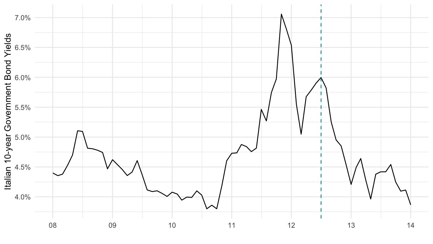
Figure 10.13: Long-Term Government Bond Yields: 10-year for Italy (Source: FRED).
At 10:00 in this video, Mario Draghi says:
The premia that are being charged on sovereign states’ borrowings. These premia have to do with default, liquidity, but they also have to do more and more with convertibility, with the risk of convertibility. To the extent that these premia have to do not with factors that are inherent to my counterparty, they come within our mandate, they come within our remit. (…) So we’ll have to cope with this financial fragmentation addressing these issues.
Required Readings
Alan Greenspan. U.S. Debt and the Greece Analogy. Wall Street Journal, June 18, 2010.
Paul Krugman, Multipliers and Reality, New York Times Blog Post, June 3, 2015.
Glutology - Say’s Law: Supply Creates its Own Demand. The Economist, August 10, 2017.
Overlapping Generations: Kicking the road down an endless road. The Economist, August 31, 2017.
Greg Mankiw, The National Debt Is Still a Problem, New York Times, June 20, 2019.
Alex Williams. “Why Don’t Rich People Just Stop Working?”, New York Times, October 17, 2019.
Note however that automatic stabilizers go against that: in problem set 6, we even saw that tax cuts sometimes can pay for themselves. However, this happens only if the multiplier is really very high (higher than 3, typically). For example, if tax cuts benefit people with high marginal propensities to consume.↩
It might seem a bit contradictory that a situation where the debt to GDP ratio goes to 0 automatically is called inefficient - this seems like a rather positive state of affairs. However, we shall see in the next chapter through the overlapping-generations model, that “dynamic inefficiency” means here that the government should in fact be taking on even more government debt, to restore an equality between \(r\) and \(g_Y\). You may also remember from Exercise 1 of problem set 4 - the solution is posted here - that an interest rate lower than the rate of growth implies that we are below the Golden Rule interest rate, so that the capital stock is too high, and consumption is too low.↩
Overlapping Generations: Kicking the road down an endless road. The Economist, August 31, 2017. https://www.economist.com/economics-brief/2017/08/31/kicking-the-can-down-an-endless-road.↩
Overlapping Generations: Kicking the road down an endless road. The Economist, August 31, 2017. https://www.economist.com/economics-brief/2017/08/31/kicking-the-can-down-an-endless-road.↩
Say’s Law: Supply Creates its Own Demand. The Economist, August 10, 2017. https://www.economist.com/economics-brief/2017/08/10/says-law-supply-creates-its-own-demand.↩
“Why Don’t Rich People Just Stop Working?”, New York Times, October 17, 2019. https://search.proquest.com/docview/2306065527/829FD4E88698484EPQ/1?accountid=14512.↩