I Problem Set 1 - Solution

I.1 Geometric Sums

Let us denote the geometric sum of interest by $S$: \[S=\sum_{i=0}^n x^i = 1+x+x^2+...+x^n.\] The trick to calculate this sum is to multiply it by $x$, which allows to get: \[xS=x+x^2+x^3+...+x^{n+1}.\] We can see that this is almost the same sum as the previous one except for the first term, which is missing, and the last term, which was absent from $S$, therefore: \[\begin{aligned} xS&=-1+1+x+x^2+...+x^n+x^{n+1}\\ xS&=-1+S+x^{n+1} \end{aligned}\] This implies (for $x\neq1$): \[1-x^{n+1}=(1-x)S \quad \Rightarrow \quad S=\frac{1-x^{n+1}}{1-x}.\]
For $S$ to have a finite value when $n \to \infty$, we need that $x^{n+1}$ stays finite. This happens when: \[\lvert x\rvert<1.\] In the knife edge case when $x=1$, the sum goes to infinity since it is then equal to $n+1$. If $x=-1$, then the sum oscillates between $1$ and $-1$ and does not have a limit when $n$ goes to infinity.
From question 1 and 2, we know that when $\lvert x\rvert<1$, $x^{n+1} \to 0$ when $n \to \infty$, and therefore: \[\sum_{i=0}^{\infty} x^i = 1+x+x^2+...+x^n+...=\frac{1}{1-x}.\]
We just factor in $x^m$ and then use the formula in question 1: \[\begin{aligned} \sum_{i=m}^n x^i &= x^m+x^{m+1}+...+x^n\\ &=x^m\left(1+x+...+x^{n-m}\right)\\ &=x^m\frac{1-x^{n-m+1}}{1-x}\\ \sum_{i=m}^n x^i &=\frac{x^m - x^{n+1}}{1-x}. \end{aligned}\]
The present discounted value of an infinite stream of incomes, which grows at rate $g=2$%, starts at $y_0=90000$, if the interest rate is $i=3$% is: \[y_0+y_0\frac{1+g}{1+i}+y_0\frac{(1+g)^2}{(1+i)^2} + ...\] Using the formula found in question 3 with $x=(1+g)/(1+i)$, we get: \[y_0+y_0\frac{1+g}{1+i}+y_0\frac{(1+g)^2}{(1+i)^2} + ...=y_0\dfrac{1}{1-\frac{1+g}{1+i}}=\frac{y_0(1+i)}{i-g}\] A numerical application gives (see Google Sheet): \[\frac{y_0(1+i)}{i-g}=\frac{90000 *(1+0.03)}{0.03-0.02}=9270000.\]

I.2 Taylor Approximations

We have: \[ (1+x)^n= \sum_{k=0}^n {{n}\choose{k}} \cdot x^k\] When $x$ is small, all the $x^k$ terms for $k\geq 2$ are negligible, and therefore: \[(1+x)^n\approx 1+{{n}\choose{1}}x=1+nx.\] If you do not know what ${n}\choose{k}$ means, that is fine too. You can prove the same result using recursion. For $n=1$, we know that $(1+x)^1=1+x$ (obviously). Assume that the approximation is true for $n$, or that $(1+x)^n \approx 1+nx$, let’s prove that it is true for $n+1$: \[ \begin{aligned} (1+x)^{n+1}&=(1+x)^n(1+x) \\ &\approx (1+nx)(1+x) \\ &\approx 1+(n+1)x + nx^2 \\ (1+x)^{n+1}&\approx 1+(n+1)x \end{aligned} \] which proves the proposition for $n+1$. Thus, the Taylor approximation is true for any $n \in \mathbb{N}$.
We have: \[(1+x)(1+y)=1+x+y+xy.\] When $x$ and $y$ are both small, then $xy$ is negligible, which gives the result: \[(1+x)(1+y)\approx1+x+y.\]
Using the formula proven in Problem 1, we get that: \[\frac{1}{1+y}=1-y+y^2-y^3+...\] When $x$ and $y$ are both small, all terms of the product are negligible except for first-order terms: \[\frac{1+x}{1+y} \approx 1+x-y.\]
Denote the price level by $p_t$ (that is, in dollars, the price of a representative basket of goods). Inflation $\pi_t$ at time $t$ is defined as the rate of growth of this price level between $t$ and $t+1$: \[\frac{p_{t+1}}{p_t}=1+\pi_t.\] If you leave one dollar at the bank, and if the nominal interest rate is given by $i_t$, then you end up at the end of the period with $1+i_t$ dollars at the bank. With this, you can buy a quantity of goods given by $(1+i_t)/p_{t+1}$. If you buy a quantity of goods at time $t$, then you get a number of goods equal to $1/p_t$. Thus, the rate of increase in your purchasing power if you leave your money in the bank is given by: \[\frac{(1+i_t)/p_{t+1}}{1/p_t}=\frac{1+i_t}{1+\pi_t}.\] An exact value for the real interest rate is thus: \[\begin{aligned} \frac{1+i_t}{1+\pi_t}-1&=\frac{1+0.01}{1+0.015}-1\\ &=-0.00492610837\\ \frac{1+i_t}{1+\pi_t}-1&= -0.492610837\%. \end{aligned}\] An approximate value from the above formula is: \[\begin{aligned} \frac{1+i_t}{1+\pi_t}-1&\approx1+i_t-\pi_t-1\\ &\approx0.01-0.015\\ \frac{1+i_t}{1+\pi_t}-1&\approx-0.5\%. \end{aligned}\] This is not such a bad approximation.

I.3 Growth Rates

Iterating on the formula: \[y_{t+1}=(1+g)y_t \quad \Rightarrow \quad y_T=(1+g)^Ty_0,\] allows to find the result: \[G = \frac{y_T}{y_0}-1=(1+g)^T-1.\]
Again, inverting the previous relation: \[G = (1+g)^T-1,\] allows to find: \[\boxed{g = \frac{y_{t+1}}{y_{t}}-1=(1+G)^{1/T}-1}.\]
Applying the previous formula allows to get (see Google Sheet): \[\begin{aligned} g &=(1+0.01)^{1/365}-1\\ &= 0.00002726155\\ g &=0.0027\% \end{aligned}\] You give up approximately $2.7 every day (your bank most likely is investing this money on your behalf, so you are rather giving this money to your bank): \[0.00002726155*100000=2.7.\]

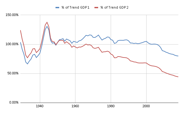
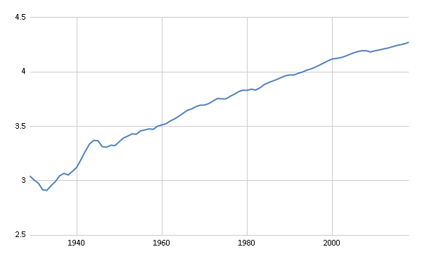
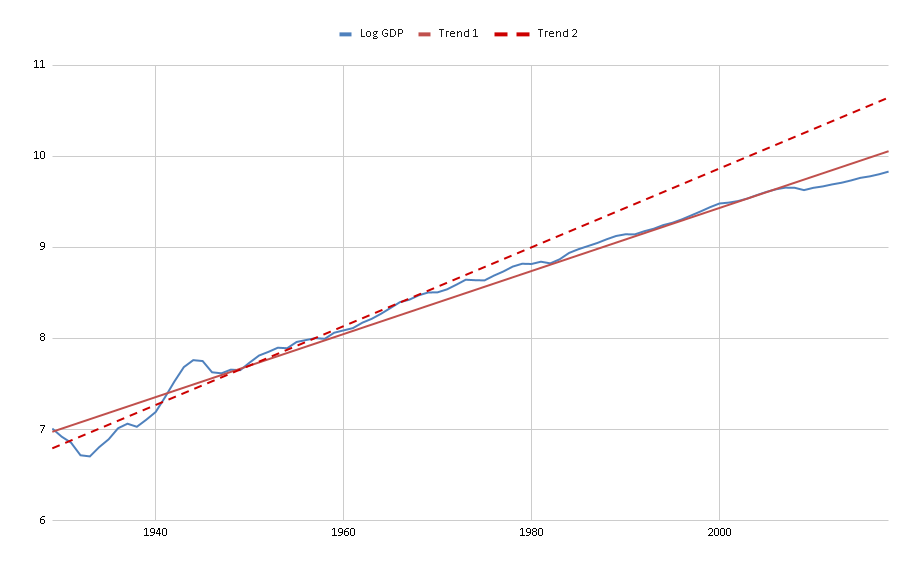
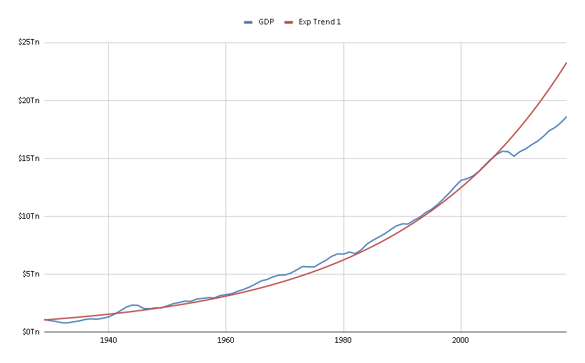
I.4 Replicating Figures 1.1, 1.2, and 1.3

See Google Sheet.

See Google Sheet.

See Google Sheet.