15 A Macroeconomic History of the U.S.

Link to slides / Link to handouts

During this concluding lecture, we will go through a very short overview of U.S.’s post 1929 macroeconomic history, around plots of various macroeconomic time series. Figure 15.1 shows the evolution of real GDP in the U.S., which we started the class with in lecture 1. We now know that the growth of real GDP over the long run is explained by the growth in technology (lecture 5), population growth, and that the U.S. likely has exhausted the possibilities brought about by capital accumulation. In lectures 4 and 10 we even have suggested that the U.S. perhaps has in fact accumulated too much capital, and that if interest rates are lower than the growth rate, public debt is perhaps not such a problematic issue after all. During this lecture, we conclude by touching upon four related topics:

• The success of Keynesian Economics following the Crash of 1929 in section 15.1.
• Post-war Macroeconomic Performance of the U.S. by party of the President in section 15.2.
• U.S. Fiscal Policy towards different income groups in section 15.3.
• A cautionary note on the potential negative effects of trade deficits created by Keynesian policies in section 15.4.

Figure 15.1: U.S. Real GDP (1929-2018) - Log Scale.

15.1 The success of Keynesian Economics

Figure 15.1 shows that overall growth in standards of leaving did not occur without ups and downs. The most evident on this picture probably is the Great Depression starting in 1929; compared to that episode, the Great Recession of 2007-2009 looks like a minor recession. I believe that one reason why the 2007-2009 financial crisis did not turn as bad as the 1929 crisis, is that an important fiscal stimulus was implemented, which prevented a further slump.

In contrast, the response to the 1929 crisis was initially very different. Figure 15.2 shows the Cyclically Adjusted Price to Earnings Ratio (CAPE) on the U.S. Stock Market from 1920 to 1942. On this graph, we can very clearly see the 1929 “Big Crash” which started the Great Depression in the United States. This crash occured at the end of October 1929, represented by the vertical dotted line on Figure 15.2: it started on October 24 (“Black Thursday”) and continued until October 29, 1929 (“Black Tuesday”).

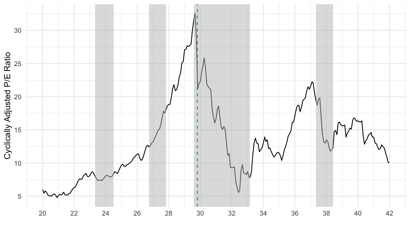
Figure 15.2: U.S. Stock Market (1920-1942).

Then U.S. president Herbert Hoover from 1929 to 1933 decided to raise taxes substantially in order to restore the balance in the budget. This policy was largely unsuccessful, and led to very high unemployment rates (higher than 20%), just as Keynesian theory predicts it would. It also led to deflation (a negative inflation rate) as shown on Figure 15.3.

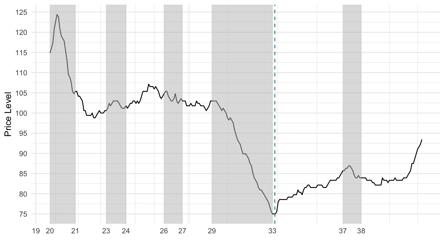
Figure 15.3: U.S. Prices (1920-1942)

In Spring 1933, Franklin D. Roosevelt left the Gold Standard (leading to a de-facto devaluation in the dollar, which was expansionary) and started a set of expansionary fiscal policies usually refered to as the “New Deal”. The dollar was famously devalued by F.D. Roosevelt, as shown on Figure 15.4.

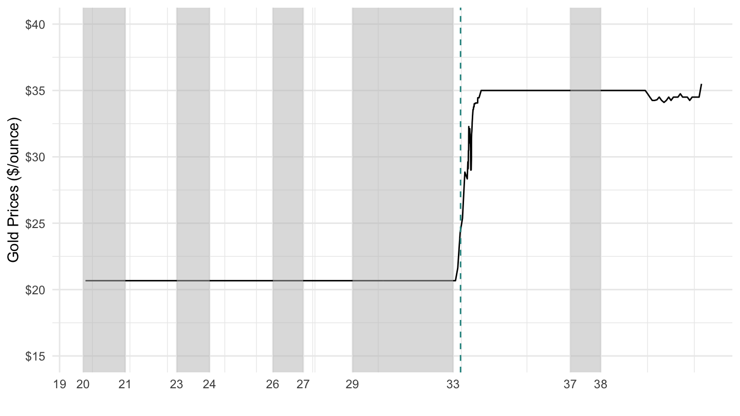
Figure 15.4: Spring 1933: FDR takes U.S. off the Gold Standard

The same discussions on whether to balance the budget or not to restore financial balance, was taking place in the United Kingdom as well. J.M. Keynes took a very active role in all these discussions - well before in fact, he started to write the General Theory. You can read many of the articles he wrote at the time in Essays in Persuasion.

Joan Robinson, in “What Has Become of the Keynesian Revolution?”, summarizes this episode:

In 1931, when the world crisis had produced a sharp increase in the deficit on the U.K. balance of payments, the appropriate remedy (approved as much by the unlucky Labour government as by the Bank of England) was to cut expenditure so as to balance the budget. These were the orthodox views that prevailed in the realm of public policy.

At the time, the Treasury View prevailed (see lecture 10 for a definition):

In those years British orthodoxy was still dominated by nostalgia for the world before 1914. Then there was normality and equilibrium. To get back to that happy state, its institutions and its policies should be restored - keep to the gold standard at the old sterling parity, balance the budget, maintain free trade and observe the strictest laissez faire in the relations of government with industry. When Lloyd George proposed a campaign to reduce unemployment (which was then at the figure of one million or more) by expenditure on public works, he was answered by the famous “Treasury View” that there is a certain amount of saving at any moment, available to finance investment, and if the government borrows a part, there will be so much the less for industry.

Joan Robinson also reminds us that Keynes was not being heard at the time. In fact, it is very disheartening that the Nazis implemented the first fiscal stimulus programs, way before Roosevelt:

Meanwhile the Nazis had been proving Lloyd George’s point with a vengeance. It was a joke in Germany that Hitler was planning to give employment in straightening the Crooked Lake, painting the Black Forest white and putting down linoleum in the Polish Corridor. The Treasury view was that his unsound policies would soon bring him down. But the little group of Keynesians was despondent and frustrated. We were getting the theory clear at last, but it was going to be too late.

Finally, before we end this class, I want to make clear that J.M. Keynes was actually trying to save capitalism from communism which then was a threatening credible alternative:

There is a kind of simpleminded Marxist who bas a great resentment against Keynes because he is held responsible for saving capitalism from destroying itself in another great slump. This is often made an excuse for not understanding the theory of effective demand, although Michal Kalecki derived pretty well the same analytical system as Keynes from Marx’s premises. Moreover it implies that capitalists are so stupid that they would fail to learn from their experiences during the war that government outlay maintains profits unless they had Keynes to point it out to them.

But what was the political tendency of the General Theory? Keynes himself described it as “moderately conservative,” but this was intended as a paradox, for the whole book is a polemic against established ideas. His own mood often swung from left to right. Capitalism was in some ways repugnant to him, but Stalinism was much worse. In his last years, certainly, the right predominated. When I teased him about accepting a peerage he replied that after sixty, one had to become respectable. But his basic view of life was aesthetic rather than political. He hated unemployment because it was stupid and poverty hecause it was ugly. He was disgusted by the commercialism of modern life. (It is true he enjoyed making money for his College and for himself but only as long as it did not take up much time.) He indulged in an agreeable vision of a world where economics has ceased to be important and our grandchildren can begin to lead a civilized life.

15.2 Post-war Macroeconomic Performance

One angle to approach the U.S. post-war macroecononomic performance is to study the economic results of different presidents based on their party of origin. In an American Economic Review article (the top scholarly publication of the economics profession), Alan Blinder and Mark Watson use time series techniques to investigate this issue scientifically.

There results are provocative. As Figures 15.5 and 15.6 show, Democratic presidents have a significantly better economic record than Republican presidents. Figure 15.7 shows that this is mostly explained by their differential macroeconomic performance in the first years of their presidency.

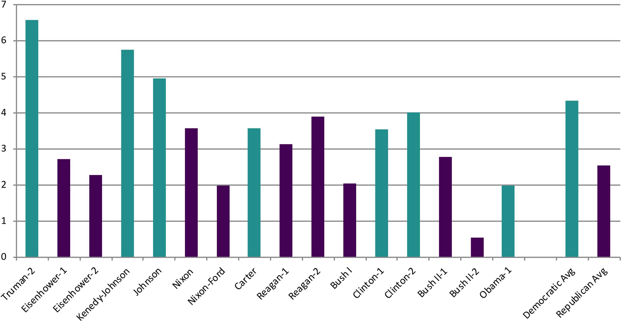
Figure 15.5: Average GDP Growth. Source: Blinder, Watson (2016).

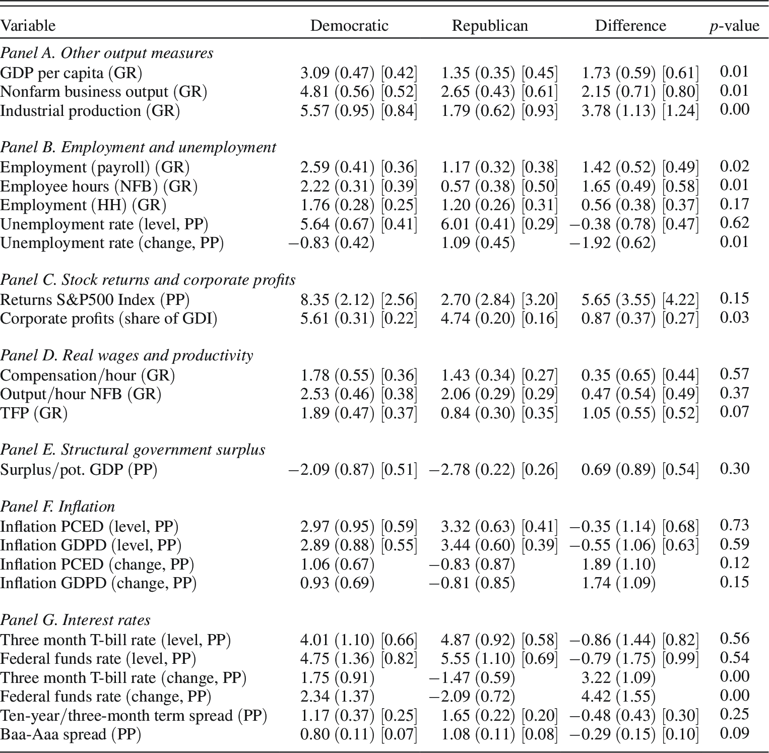
Figure 15.6: Average Values of Macroeconomic Variables by Party of President. Source: Blinder, Watson (2016).

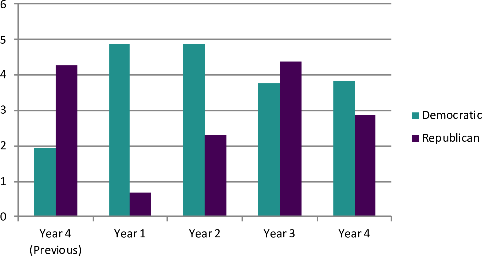
Figure 15.7: Growth Rates by Year, Within Presidential Terms. Source: Blinder, Watson (2016).

However, Alan Blinder and Mark Watson also investigate the source of this difference, using the various variables that are typically thought to be associated to good macroeconomic performance. They conclude that:

The answer is not found in technical time series matters nor in systematically more expansionary monetary or fiscal policy under Democrats. Rather, it appears that the Democratic edge stems mainly from more benign oil shocks, superior total factor productivity (TFP) performance, a more favorable international environment, and perhaps more optimistic consumer expectations about the near-term future.

This result should be apparent on Panel E of Figure 15.9. This shows that the Romer and Romer (2010) tax series presented in Lecture 14 does not explain the relative performance of Democrats versus Republicans. Note however that these results do not account for the differential impacts of taxes on high income and low income earners shown by Zidar (2018), which we looked at in lecture 14. Figure 15.10 decomposes the Romer and Romer (2010) tax series between the top 10% and the bottom 90%.

Another important factor cited by Blinder and Watson is the differential impact of oil shocks, shown on Figure 15.8.

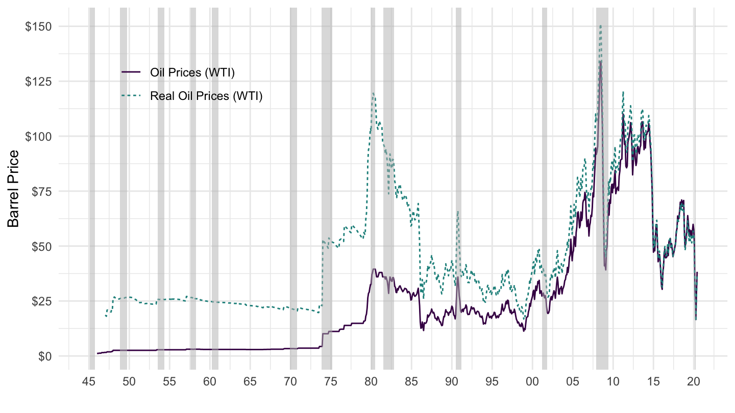
Figure 15.8: Oil Prices (1970-2019)

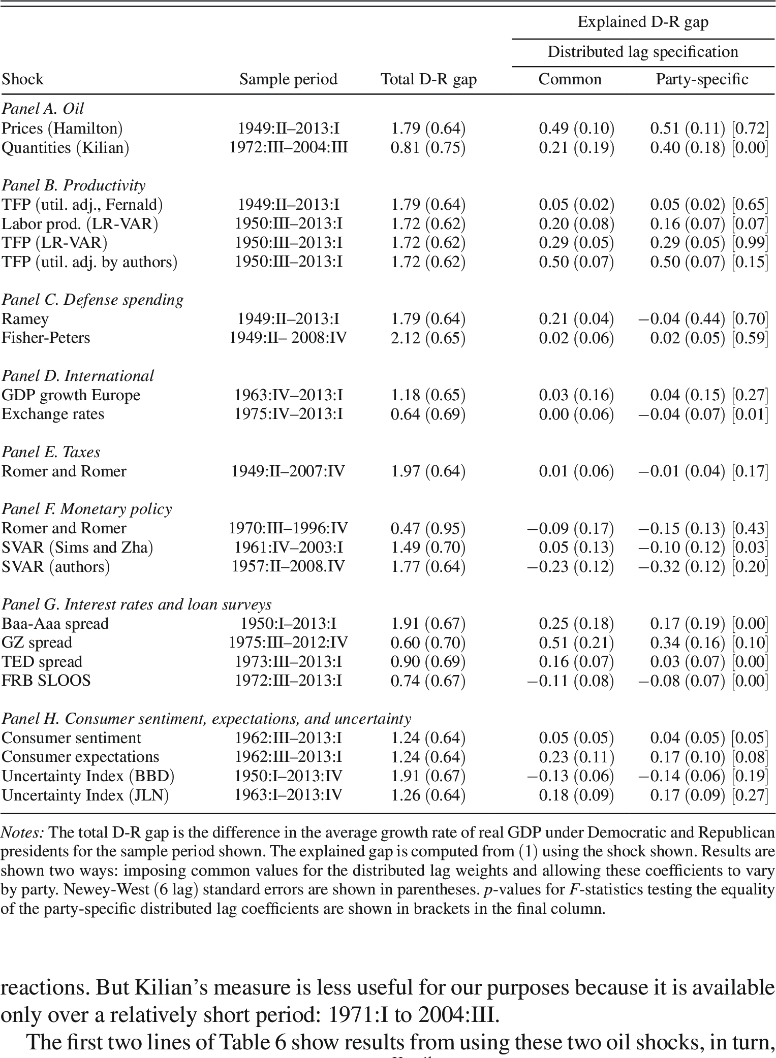
Figure 15.9: Explaining the Democrat-Republican Growth Gap. Source: Blinder, Watson (2016).

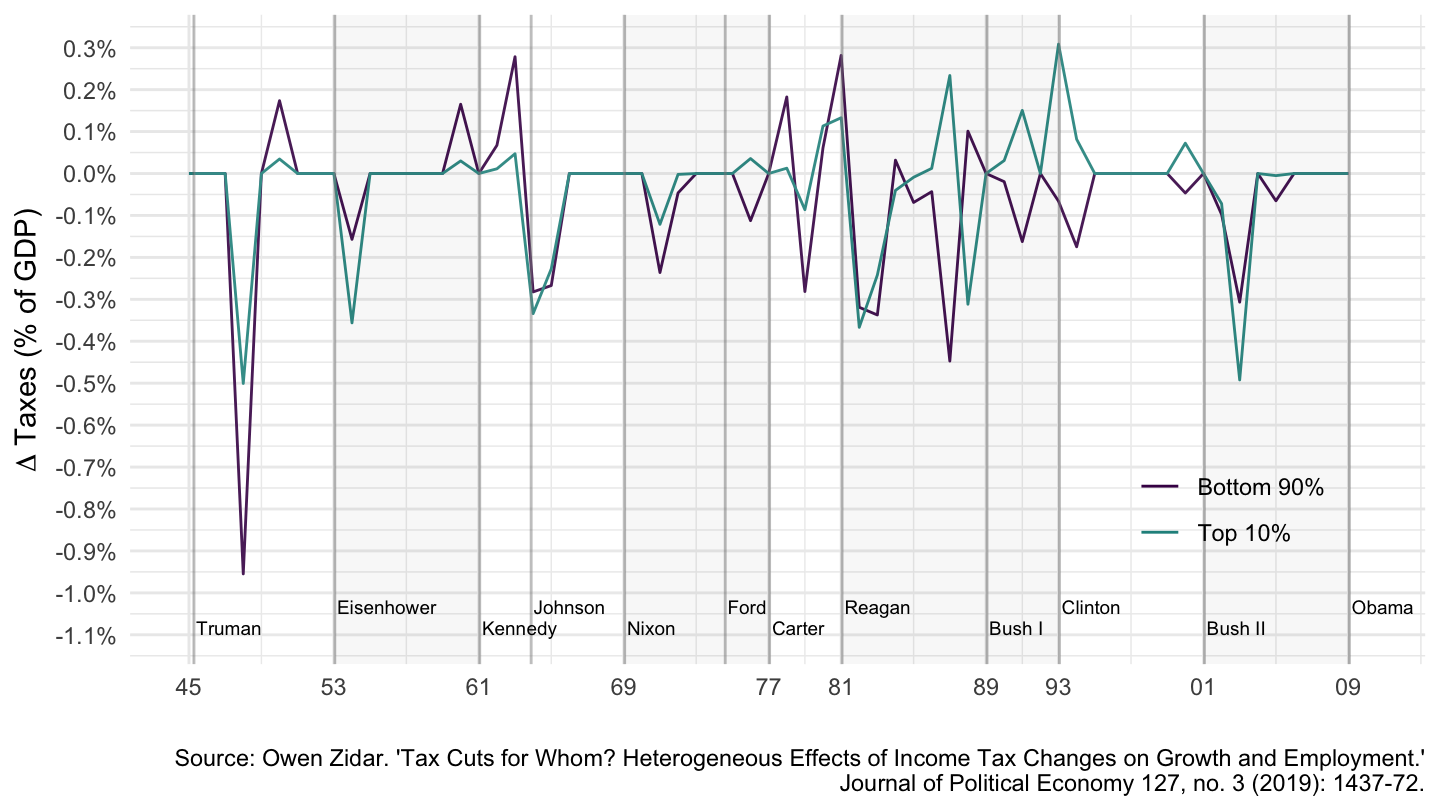
Figure 15.10: Decomposing the Romer and Romer (2010) Aggregate Tax Changes into Top 10% and Bottom 90%. Source: Zidar (2019).

15.3 U.S. Fiscal Policy

As we saw in lecture 9, fiscal policy is an important factor to take into account if we want to understand macroeconomic policy. In particular, it is important to look at the change in fiscal policy for different (pre-tax) income groups:

• Average tax rates for Top 1% and the Bottom 50%. (Figure 15.11)
• Average tax rates for the Top 10% and the Bottom 90%. (Figure 15.12)
• Average tax rates for the Top 1%, the Top 0.5%, and the Top 0.01%. (Figure 15.13)
• Top Marginal tax rates. (Figure 15.14)

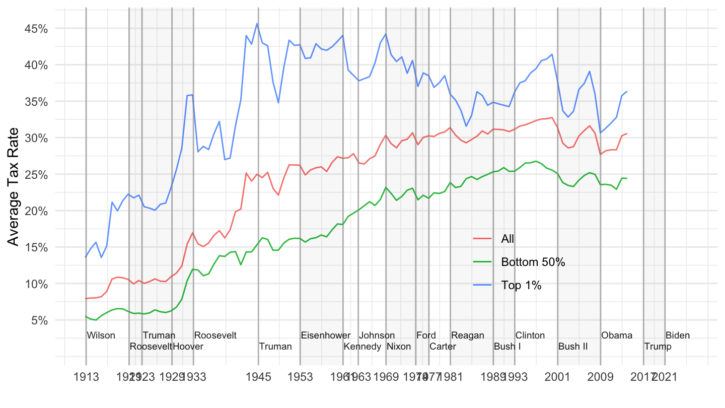
Figure 15.11: Average tax rates: Top 1%, Bottom 50%. Source: Piketty et al. (2017).

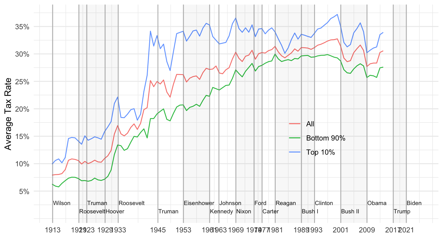
Figure 15.12: Average tax rates: Top 10%, Bottom 90%. Source: Piketty et al. (2017).

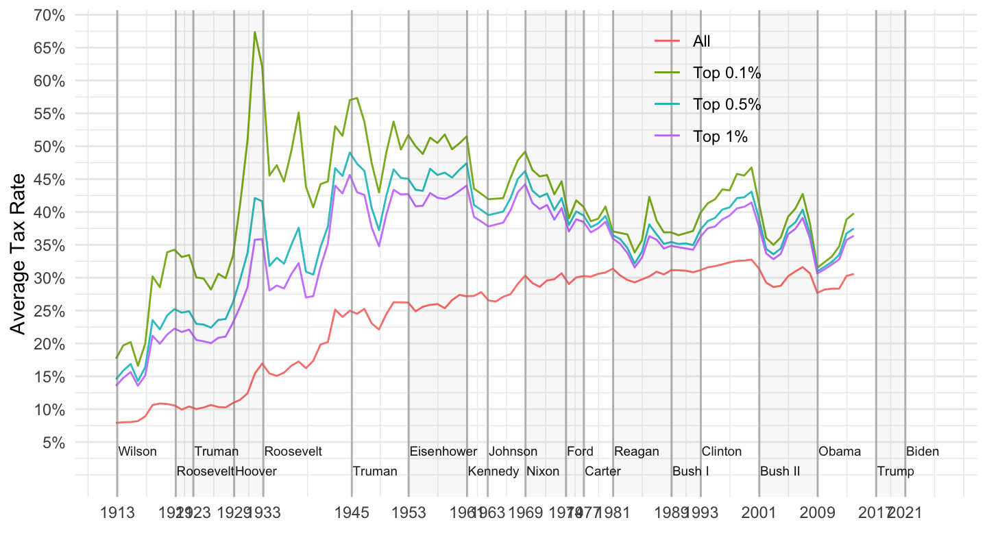
Figure 15.13: Average tax rates: Top 1%, Top 0.5%, Top 0.1%. Source: Piketty et al. (2017).

Figure 15.14: Top Marginal Tax Rates. Source: Piketty et al. (2014).

15.4 Trade Deficits and Manufacturing Decline

I shall conclude this class on a cautionary tale on aggregate demand stimulating policies. As we have seen in lecture 11, these policies have the unintended consequence of raising the U.S. trade deficit.

Although many economists usually take a benign view of trade deficits in general, and deindustrialization in particular, I am more agnostic. Trade deficits distort the structure of production towards services, as to a first approximation only goods can be imported. The negative consequences of the fall in the manufacturing sector has hurt some communities substantially, and may largely explain the rise of Donald Trump.

This section presents some evidence in this direction.

Figures 15.15 and ?? show the growing trade deficit since the 1980s, which occurred whether or not there was a budget deficit. In 1993-2001, the progressivity of the tax system was substantially increased, which led to an improvement in the fiscal situation, but also to an overall boost in aggregate demand, increasing the trade deficit further.

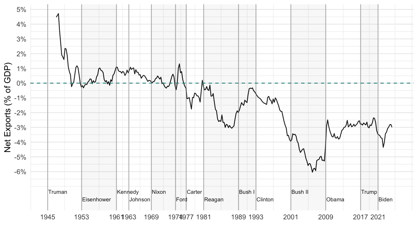
Figure 15.15: Net Exports (% of GDP).

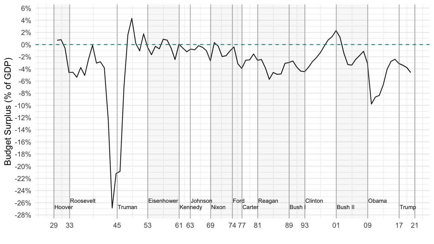
Figure 15.16: Budget Surplus, 1929-2019 (% of GDP).

Why should we potentially care about growing trade deficits, and a shrinking manufacturing sector? Paul Krugman gave the arguments of people worried about the U.S. trade deficit in a 1994 Foreign Affairs article titled “Competitiveness: A Dangerous Obsession”:

In a recent article published in Japan, Lester Thurow explained to his audience the importance of reducing the Japanese trade surplus with the United States. U.S. real wages, he pointed out, had fallen six percent during the Reagan and Bush years, and the reason was that trade deficits in manufactured goods had forced workers out of high-paying manufacturing jobs into much lower-paying service jobs. This is not an original view; it is very widely held. But Thurow was more concrete than most people, giving actual numbers for the job and wage loss. A million manufacturing jobs have been lost because of the deficit, he asserted, and manufacturing jobs pay 30 percent more than service jobs.

Both numbers are dubious. The million-job number is too high, and the 30 percent wage differential between manufacturing and services is primarily due to a difference in the length of the workweek, not a difference in the hourly wage rate. But let’s grant Thurow his numbers. Do they tell the story he suggests? The key point is that total U.S. employment is well over 100 million workers. Suppose that a million workers were forced from manufacturing into services and as a result lost the 30 percent manufacturing wage premium. Since these workers are less than 1 percent of the U.S. labor force, this would reduce the average U.S. wage rate by less than 1/100 of 30 percent?that is, by less than 0.3 percent. This is too small to explain the 6 percent real wage decline by a fac tor of 20.

One reason is that manufacturing jobs provide high-paying jobs for people who did not go to college. Jobs in the service sector are, in contrast, not as well paid. If you want the opposite side of the argument, you should read “Competitiveness: A Dangerous Obsession” by Paul Krugman, or his book on the topic “Pop Internationalism” (see the references below).

J.M. Keynes was in fact very aware of that risk, and was taking it more seriously than most mainstream contemporary economists (one exception is Dani Rodrik, at Harvard University). For that reason, J.M. Keynes’ preference was often going back and forth between free trade and protection.⁴⁸

In Proposals for a Revenue Tariff, included in Essays in Persuasion he was arguing in favor of a revenue tariff:

But the main decision which seems to me to-day to be absolutely forced on any wise Chancellor of the Exchequer, whatever his beliefs about Protection, is the introduction of a substantial revenue tariff. It is certain that there is no other measure all the immediate consequences of which will be favourable and appropriate. The tariff which I have in mind would include no discriminating protective taxes, but would cover as wide a field as possible at a flat rate or perhaps two flat rates, each applicable to wide categories of goods.

The reason, for him, was to prevent a further trade deficit:

I am of the opinion that a policy of expansion, though desirable, is not safe or practicable to-day, unless it is accompanied by other measures which would neutralise its dangers. Let me remind the reader what these dangers are. There is the burden on the trade balance, the burden on the Budget, and the effect on confidence. If the policy of expansion were to justify itself eventually by increasing materially the level of profits and the volume of employment, the net effect on the Budget and on confidence would in the end be favourable and perhaps very favourable. But this might not be the initial effect.

He added:

Compared with any alternative which is open to us, this measure is unique in that it would at the same time relieve the pressing problems of the Budget and restore business confidence. I do not believe that a wise and prudent Budget can be framed today without recourse to a revenue tariff. But this is not its only advantage. In so far as it leads to the substitution of home-produced goods for goods previously imported, it will increase employment in this country. At the same time, by relieving the pressure on the balance of trade it will provide a much-needed margin to pay for the additional imports which a policy of expansion will require and to finance loans by London to necessitous debtor countries. In these ways, the buying power which we take away from the rest of the world by restricting certain imports we shall restore to it with the other hand. Some fanatical Free Traders might allege that the adverse effect of import duties on our exports would neutralise all this; but it would not be true.

Regardless of one’s view on the issue of declining manufacturing employment, it is a fact that, at least since 2000, manufacturing employment has been fast declining as shown on Figure 15.17. The worry about U.S. trade deficits and competitiveness dates back to much before 2000, in fact. As early as 1971, Nixon was saying:⁴⁹

How are we going to compete, and how are we going to add 20 million jobs? We’ve made a national decision that we can’t compete in making cars, or making steel, or making airplanes. So are we going to end up just making toilet paper and toothpaste?

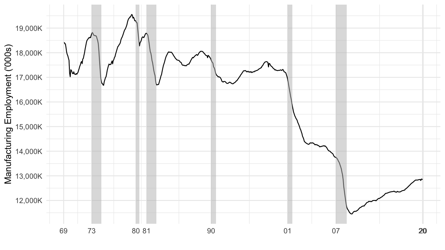
Figure 15.17: Manufacturing Employment (In Thousands)

I will end the with four pictures, which to my mind suggest a potential problem with the decline in manufacturing employment, linked to aggregate demand stimulating policies. To me, these potential issues may explain the rise of Donald Trump, and his election.

• Figure 15.18 shows the employment rate of prime-age individuals. You can see that the employment of non-college men has fallen by approximately 5 percentage points since 1980.

• Figure 15.19 shows monthly U.S. Employment in millions. Manufacturing employment has steadily fallen from 1980 to 2015, but before the 2007-2009 financial crisis, construction employment was rising and somewhat compensating the decline in manufacturing.

• Figure 15.20 plots the construction, manufacturing, and nonemployment shares of employment for noncollege men. It shows that during the 2000s boom, the construction sector masked the decline in manufacturing sector, as many noncollege men went to construction instead of manufacturing. Obviously, this state of affairs ended with the financial crisis in 2007-2009.

• Figure 15.21 shows the relationship between manufacturing decline and the opioid crisis. Regions which were most hurt by the decline in manufacturing are those where the opioid crisis is more severe. Other studies have shown a link between the fall in manufacturing employment and the rise of Donald Trump.

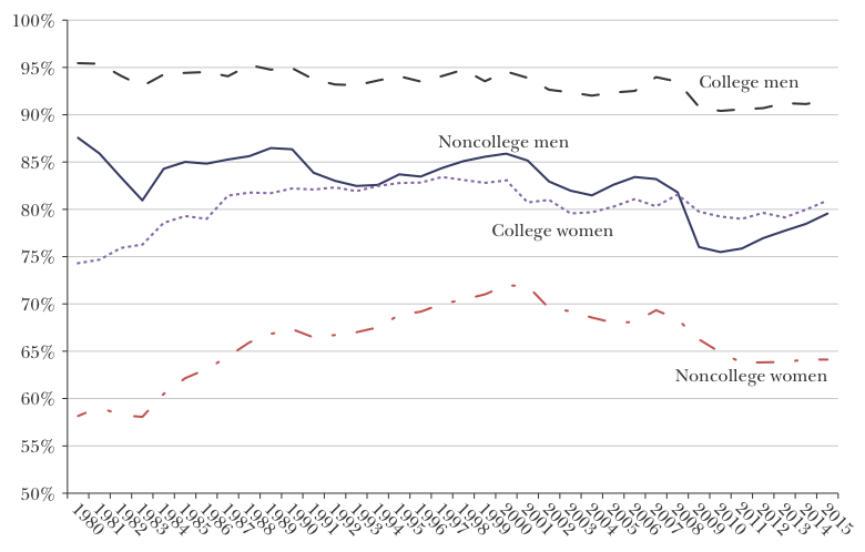
Figure 15.18: Employment Rate, Prime-Age Individuals, 1980–2015. Source: Charles et al. (2016).

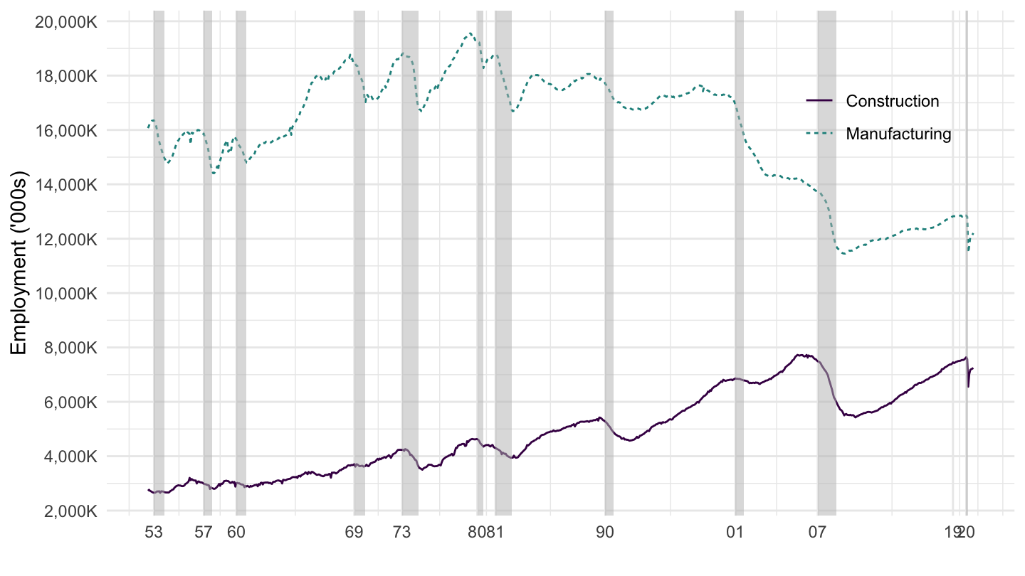
Figure 15.19: Manufacturing and Construction Employment (In Thousands)

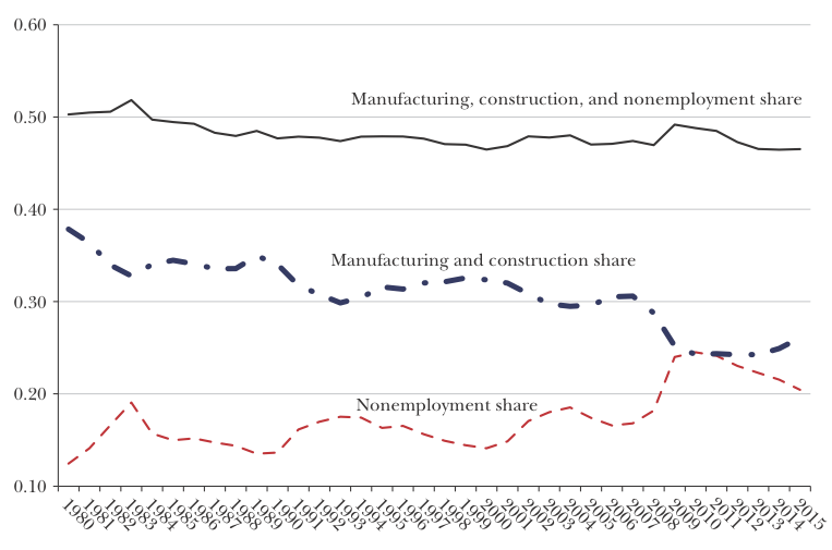
Figure 15.20: Construction, Manufacturing, and Nonemployment Shares, Noncollege Men. Source: Charles et al. (2016).

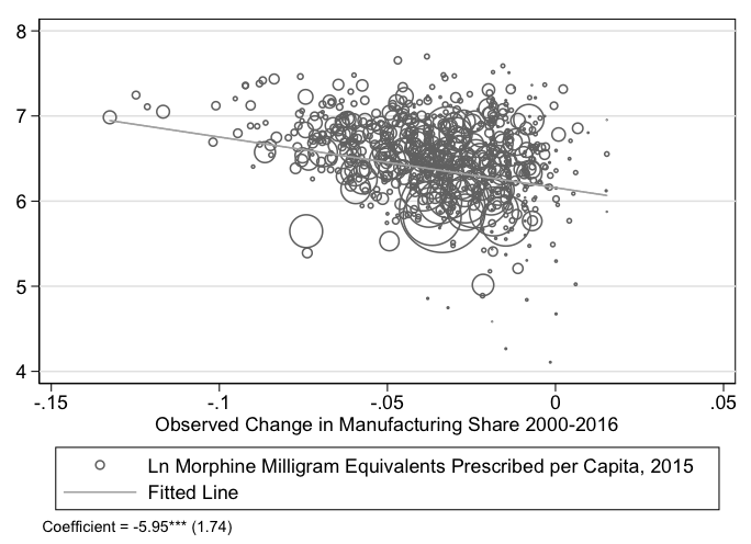
Figure 15.21: Manufacturing Decline and Opioid Crisis. Source: Charles et al. (2018).

Again, if you want to read the arguments of those who think that trade deficits are not a problem, I strongly encourage you to read both Paul Krugman’s 1994 article in Foreign Affairs, as well as his book “Pop Internationalism.” In my opinion, the issues related to aggregate demand stimulating policies’ impact on the trade balance are here to stay. Time will tell.

Additional Readings

Paul A. Samuelson. Economics: An Introductory Analysis. First Edition. Chapter 17: The Business Cycle.

J.M. Keynes, Essays in Persuasion (Springer, 1931).

Barry Eichengreen, “Keynes and Protection,” The Journal of Economic History 44, no. 2 (1984): 363–73.

(Book) Paul R. Krugman, Pop Internationalism (MIT Press, 1997).

Alan S. Blinder and Mark W. Watson, “Presidents and the US Economy: An Econometric Exploration,” American Economic Review 106, no. 4 (April 2016): 1015–45.

Kerwin Kofi Charles, Erik Hurst, and Matthew J. Notowidigdo, “The Masking of the Decline in Manufacturing Employment by the Housing Bubble,” Journal of Economic Perspectives 30, no. 2 (May 2016): 179–200.

Kerwin Kofi Charles, Erik Hurst, and Mariel Schwartz, “The Transformation of Manufacturing and the Decline in U.S. Employment,” Working Paper (National Bureau of Economic Research, March 2018).