1 Introduction to Macroeconomics
Link to slides / Link to handouts
Macroeconomics is mostly concerned with explaining the level of aggregate economic activity, both in the long-run and in the short-run. Gross Domestic Product (GDP) is the value of all final goods and services produced in a country within a given period. There are two ways to think about GDP, as well as to measure it: the product approach and the income approach to GDP.
According to the product approach to GDP, GDP is the sum of four components:
- Consumption spending by households (C).
- Investment spending by households and corporations (I).
- Government purchases (G).
- Net exports (NX).
On the supply side, the production of output involves the use of factors of production, typically limited to capital (\(K\)) and labor (\(L\)). These factors of production receive payment for their use, whose sum equals GDP. The income approach to GDP consists in dividing up these payments into the different factors of production. Again, this often simply means a division of total value added into capital income, and labor income. It is presented in section 1.8. An implicit assumption here is that there are no “rents” in the economy, that is that nothing can be obtained without either labor or capital. This is not exactly true, as for example oil is clearly more valuable than the costs of extracting it from the soil. Land is another example of something that is preexisting, but nevertheless earns a payment (over and above what is needed to maintain land). It is a good first-order approximation however, as most production in fact requires either labor or capital.
1.1 Data on GDP - Trends and Cycles
| Period | Growth |
|---|---|
| 1929-1945 | 5.01% |
| 1945-1971 | 2.86% |
| 1971-1990 | 3.26% |
| 1990-2019 | 2.44% |
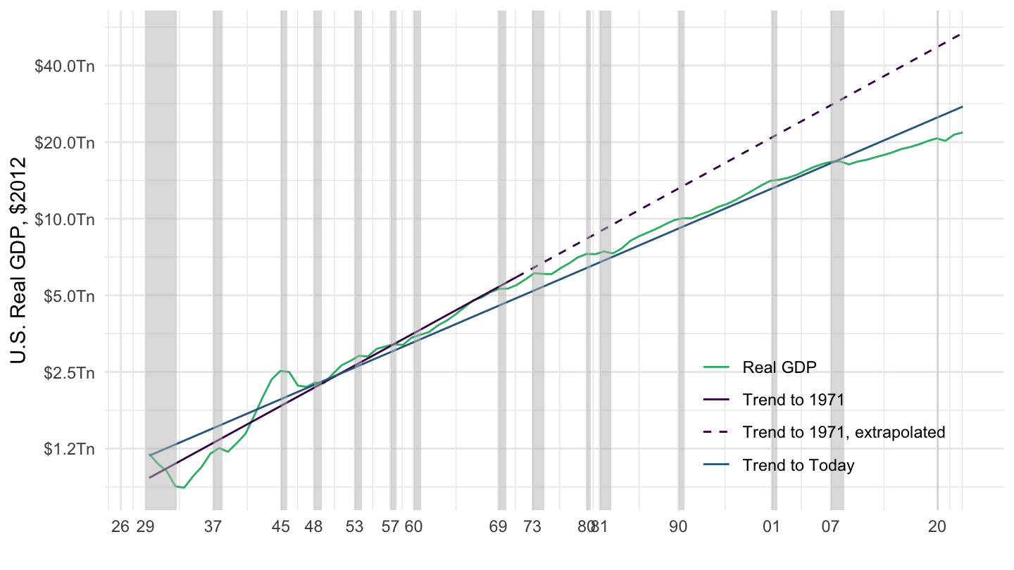
Figure 1.1: U.S. Real GDP Trends (1929-2019) - Log Scale.
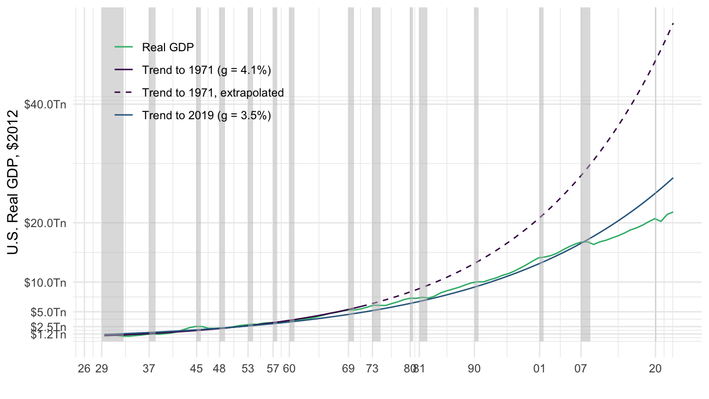
Figure 1.2: U.S. Real GDP Trends (1929-2019).
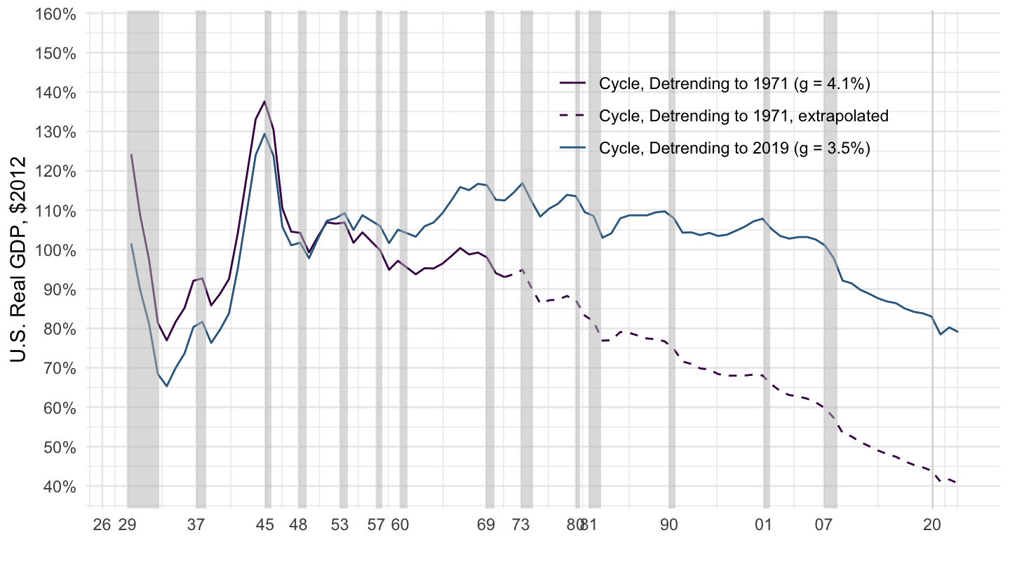
Figure 1.3: U.S. Real GDP Cycles (1929-2019).
1.2 The Product Approach to GDP
GDP is equal to the total aggregate demand for goods: \[ Y = C + I + G + X -M.\] We often define net exports as:3 \[NX \equiv X-M,\] so that GDP is simply: \[ Y = C + I + G + NX.\]
Figure 1.4 plots GDP (in dollars) from the National Income and Product Accounts (NIPA) produced by the Bureau of Economic Analysis (BEA), in billions of dollars. Shaded areas correspond to U.S. Recessions as defined by the National Bureau of Economic Research (NBER) - part of the task of macroeconomics is to explain why recessions occur, so we shall of course come back to this issue of defining and explaining recessions. This is not the most compelling way to represent the time series of GDP, however, because the benchmark is exponential growth for GDP. Therefore, Figure 1.5 represents the time series of GDP using a logarithmic scale for the y-axis. This representation allows to see that GDP grows approximately linearly over time, although average growth has slowed down recently. It’s much harder to see this with a linear scale, which is why you should definitely use log scales when plotting exponential processes. (Note that many economists still don’t although they should !)
Macroeconomics is mostly concerned with explaining the level of aggregate economic activity, both in the long-run and in the short-run. Gross Domestic Product (GDP) is the value of all final goods and services produced in a country within a given period. There are two ways to think about GDP, as well as to measure it:
- According to the product approach to GDP, GDP is the sum of four components:
- Consumption spending by households (C).
- Investment spending by households and corporations (I).
- Government purchases (G).
- Net exports (NX).
- On the supply side, the production of output involves the use of factors of production, typically limited to capital (\(K\)) and labor (\(L\)). These factors of production receive payment for their use, whose sum equals GDP. The income approach to GDP consists in dividing up these payments into the different factors of production. Again, this often simply means a division of total value added into capital income, and labor income. It is presented in section 1.8. An implicit assumption here is that there are no “rents” in the economy, that is that nothing can be obtained without either labor or capital. This is not exactly true, as for example oil is clearly more valuable than the costs of extracting it from the soil. Land is another example of something that is preexisting, but nevertheless earns a payment (over and above what is needed to maintain land). It is a good first-order approximation however, as most production in fact requires either labor or capital.
In theory, both the product and the income approach to GDP should lead to the same results. In practice, there is usually a (small) discrepancy between the two.
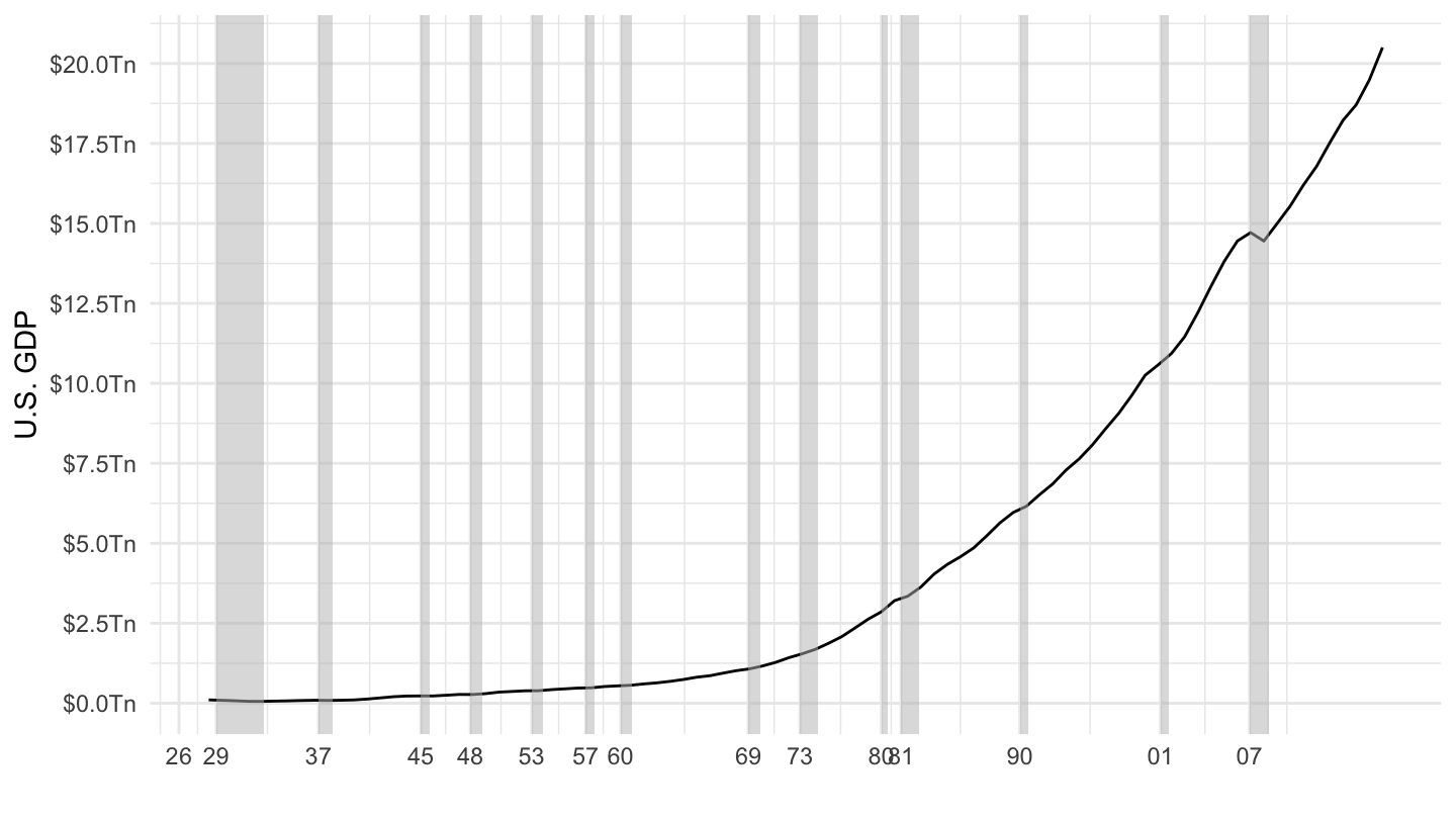
Figure 1.4: U.S. GDP (1929-2019).
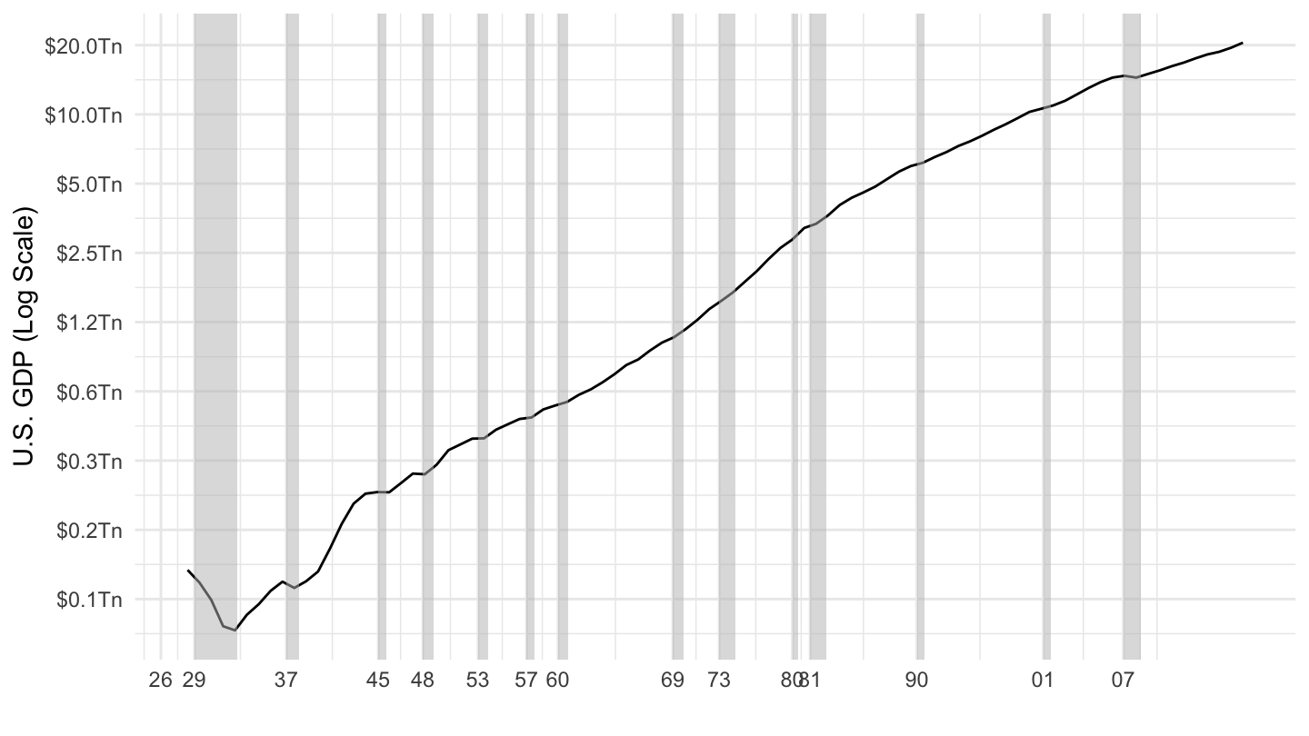
Figure 1.5: U.S. GDP (1929-2019) - Log Scale.
You should notice on this graph that nominal GDP appears to grow particularly rapidly in the 1970s, a period in which the U.S. economy was experiencing two oil shocks in 1973 and 1979, and was not particularly growing very fast. For this reason, economists usually focus on real GDP instead, as on Figures 1.6 and 1.7. On Figure 1.7 in particular, you can note that indeed, the 1970s were not a period of particularly strong growth.
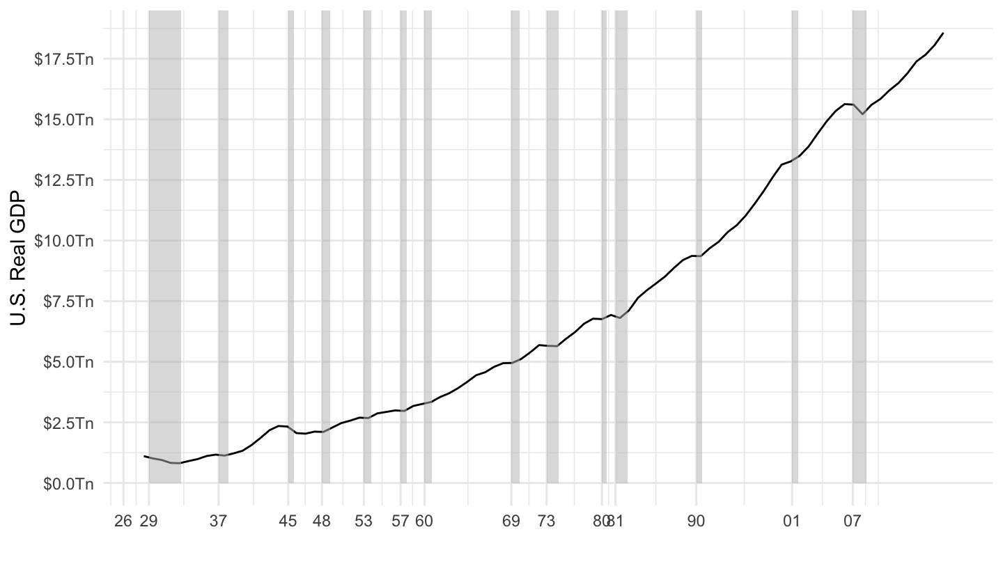
Figure 1.6: U.S. Real GDP (1929-2019).
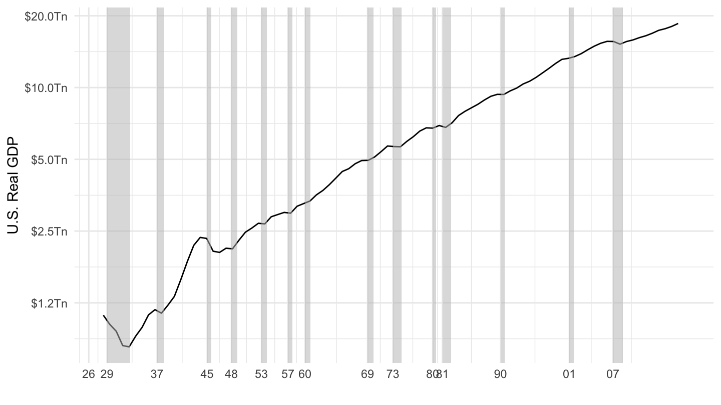
Figure 1.7: U.S. Real GDP (1929-2019) - Log Scale.
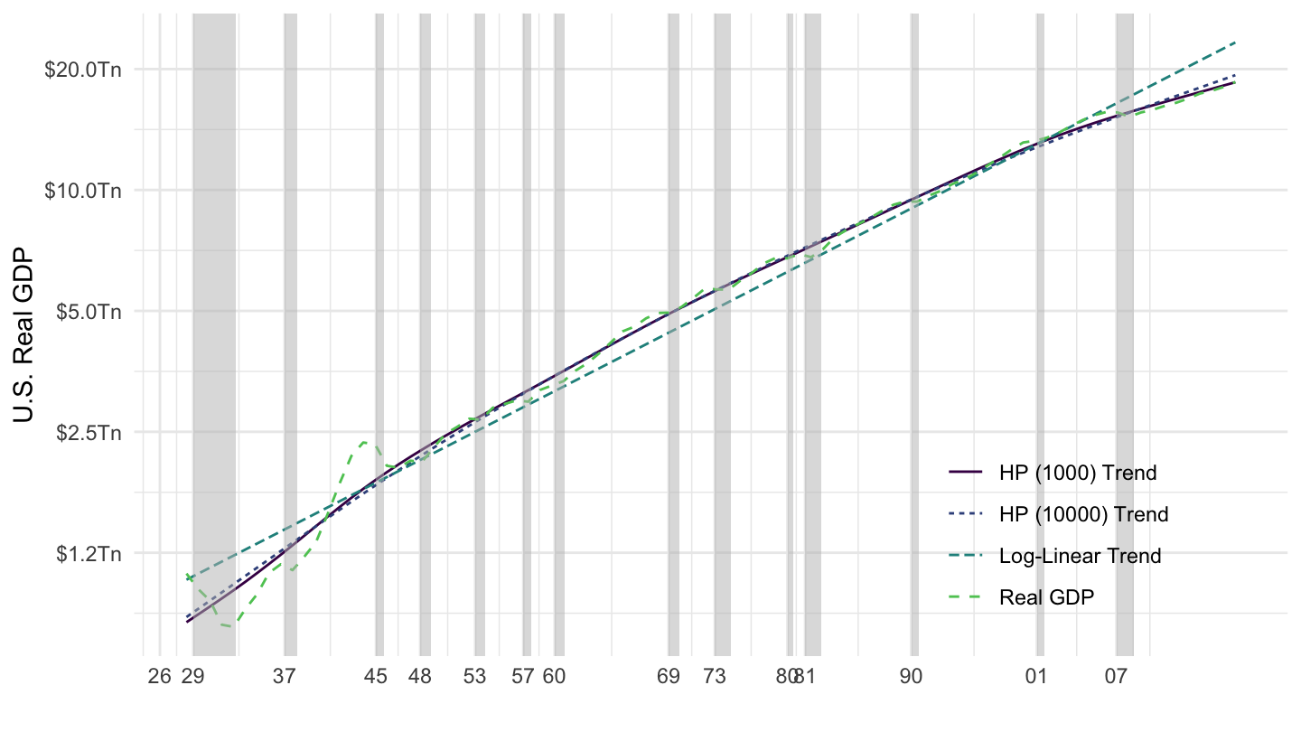
Figure 1.8: U.S. Real GDP Trends (1929-2019) - Log Scale.
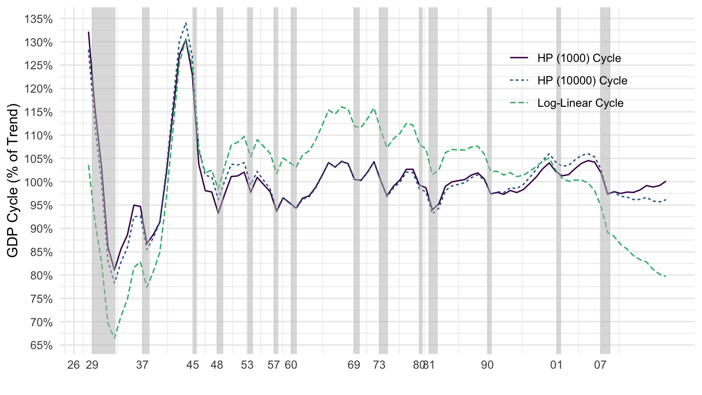
Figure 1.9: U.S. Real GDP Cycle (1929-2019).
We now examine each component of aggregate demand in turn:
- Consumption (C).
- Investment (I).
- Government Purchases (G).
- Net Exports (NX).
The data is available here, and the data is scaled by GDP in Table 1.2.
| Description | 1929 | 1960 | 1990 | 2017 |
|---|---|---|---|---|
| Gross domestic product | 100% | 100% | 100% | 100% |
| Personal consumption expenditures | 74% | 61.1% | 63.9% | 68.2% |
| Goods | 41.9% | 32.6% | 25% | 21.3% |
| Durable goods | 9.4% | 8.4% | 8.3% | 7.2% |
| Nondurable goods | 32.5% | 24.2% | 16.7% | 14.1% |
| Services | 32.1% | 28.4% | 38.9% | 46.9% |
| Gross private domestic investment | 16.4% | 15.9% | 16.7% | 17.3% |
| Fixed investment | 14.9% | 15.3% | 16.4% | 17.1% |
| Nonresidential | 11.1% | 10.4% | 12.4% | 13.2% |
| Structures | 5.3% | 3.6% | 3.4% | 3% |
| Equipment | 5.3% | 5.5% | 6.2% | 5.9% |
| Intellectual property products | 0.6% | 1.3% | 2.8% | 4.4% |
| Residential | 3.9% | 5% | 4% | 3.9% |
| Change in private inventories | 1.5% | 0.6% | 0.2% | 0.2% |
| Net exports of goods and services | 0.4% | 0.8% | -1.3% | -2.9% |
| Exports | 5.7% | 5% | 9.3% | 12.1% |
| Goods | 5.1% | 3.8% | 6.8% | 7.9% |
| Services | 0.6% | 1.2% | 2.5% | 4.2% |
| Imports | 5.3% | 4.2% | 10.6% | 15% |
| Goods | 4.3% | 2.8% | 8.5% | 12.2% |
| Services | 1% | 1.4% | 2% | 2.8% |
| Govt Cons. Expend. and Gross Inv. | 9.2% | 22.2% | 20.8% | 17.5% |
| Federal | 1.8% | 13.4% | 9.4% | 6.5% |
| National defense | 1% | 11.2% | 6.8% | 3.8% |
| Nondefense | 0.8% | 2.2% | 2.6% | 2.7% |
| State and local | 7.4% | 8.8% | 11.3% | 11% |
1.3 Product Approach: Consumption
Figure 1.10 plots Personal Consumption Expenditures (PCE), as well as GDP (for comparison), in billions of dollars. You can see that the growth of GDP and consumption are both roughly exponential over time, because both look almost linear when plotted on a log scale (for the y-axis). In fact, consumption is an approximately constant share of GDP.
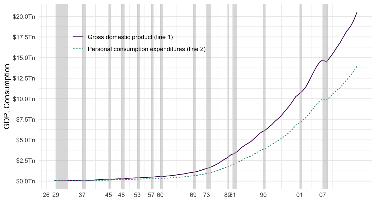
Figure 1.10: US GDP and Consumption from NIPA (BEA).
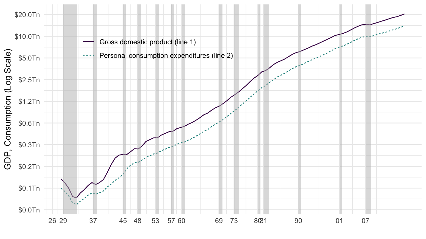
Figure 1.11: US GDP and Consumption from NIPA (BEA) - Log Scale.
To get a better of sense of how big consumption is as a fraction to GDP (although you may eyeball it on this picture), we might plot consumption as a function of GDP, which is what I do on Figure 1.12. You can see that Personal Consumption Expenditures are approximately 60 to 70 % of GDP. You can also see that it has been rising since the beginning of the 1970s. We shall also discuss that.
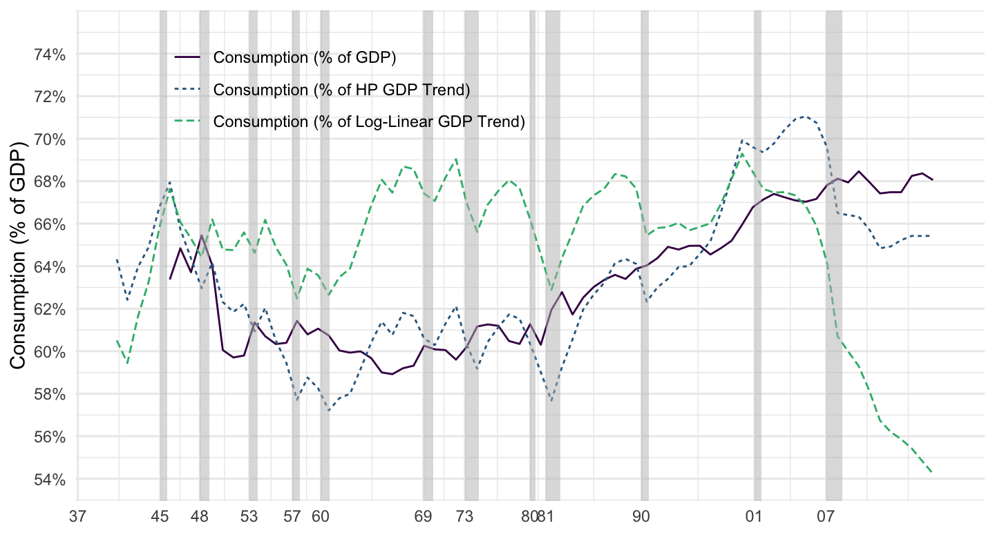
Figure 1.12: Consumption.
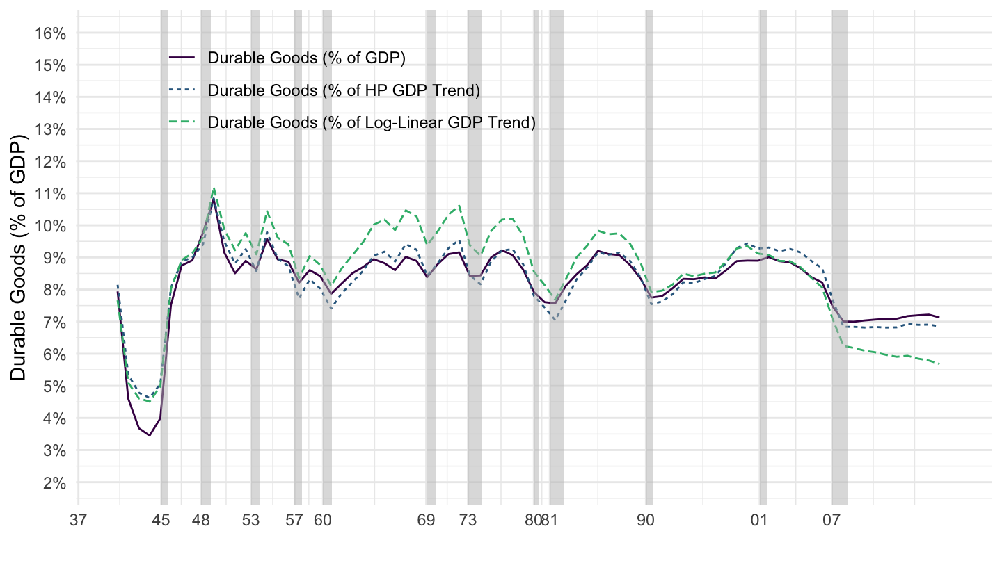
Figure 1.13: Durables Goods.
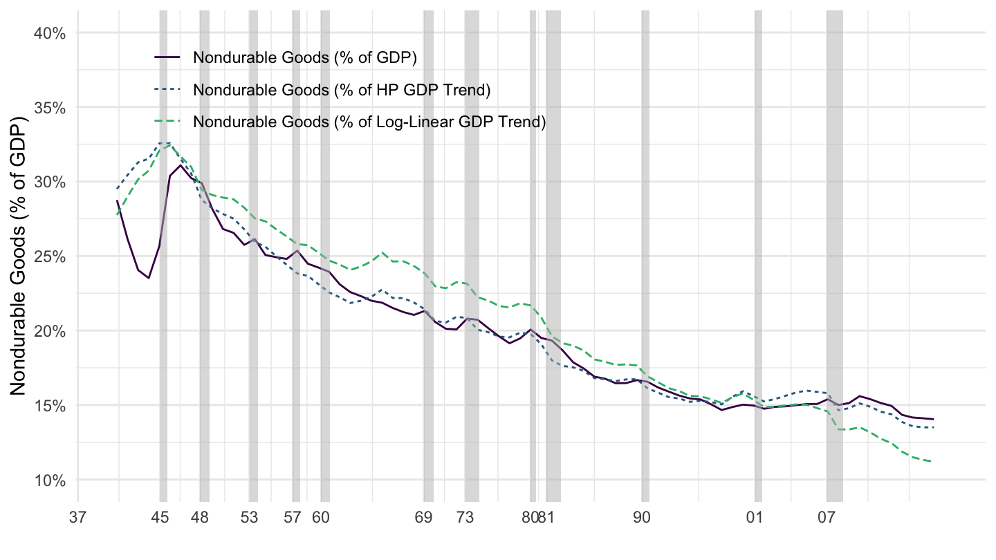
Figure 1.14: Nondurable Goods.
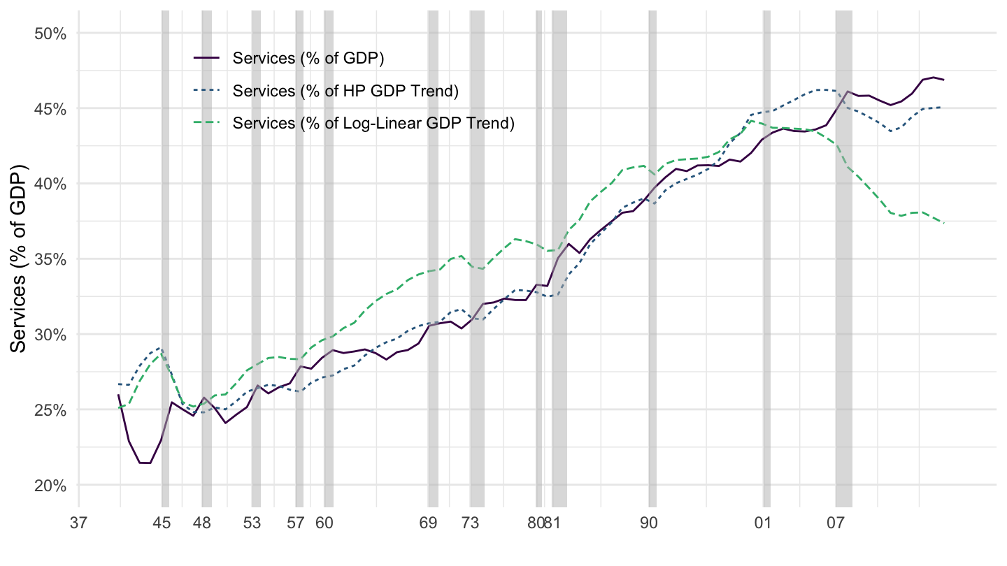
Figure 1.15: Services.
In turn, Personal Consumption Expenditures are composed of goods and services:
- Durable goods (by definition, more than 3 years of durability): for example, cars.
- Non-durable Goods (less than 3 years of durability).
- Services.
Services have become more important than goods in total consumption since the 1970s, as Figure 1.16 shows.
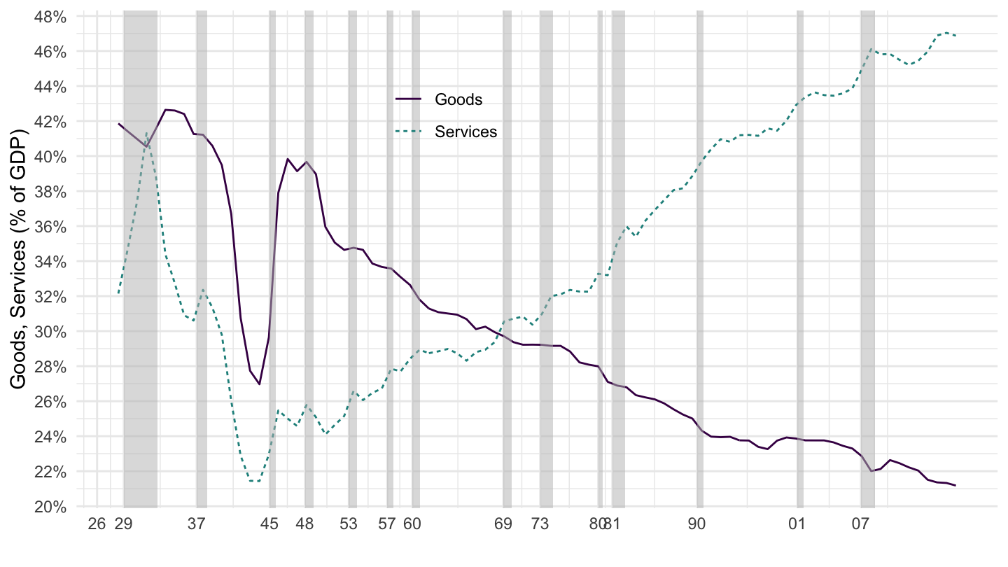
Figure 1.16: Goods and Services Consumption.
1.4 Product Approach: Investment
Investment has two components:
- non residential investment is the purchase of new capital goods by firms: structures, new plants.
- residential investment is the purchase of new houses.
Gross private domestic investment is approximately 15 to 20 % of GDP, as you can see on Figure 1.17. It is also very volatile over the cycle.
1.5 Investment
Investment. Investment.
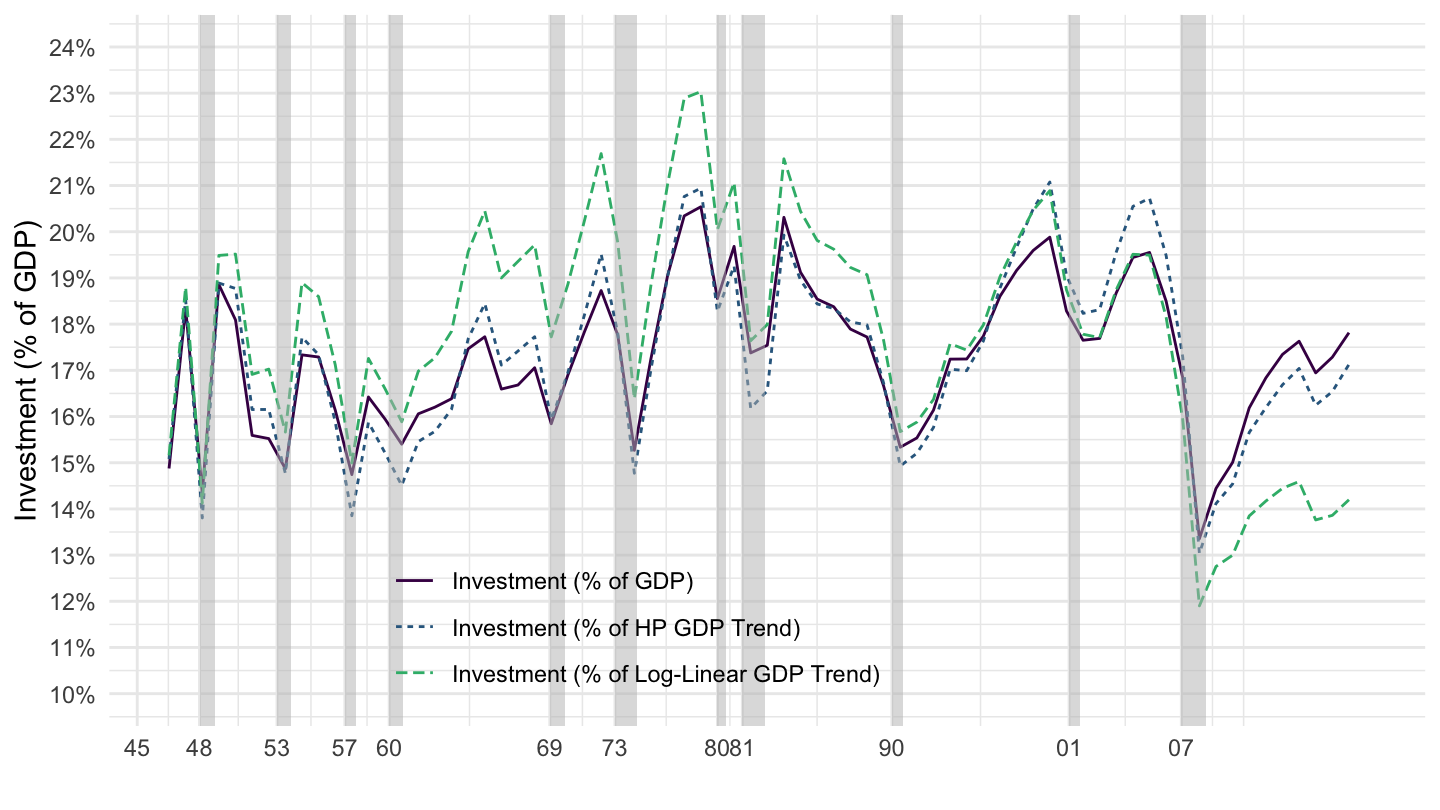
Figure 1.17: Investment.
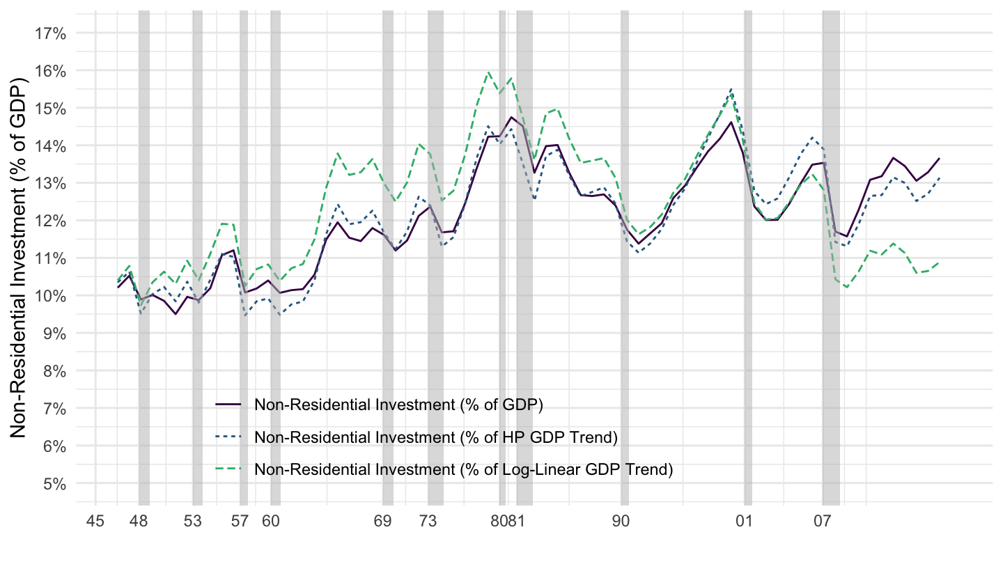
Figure 1.18: Non-Residential Investment.
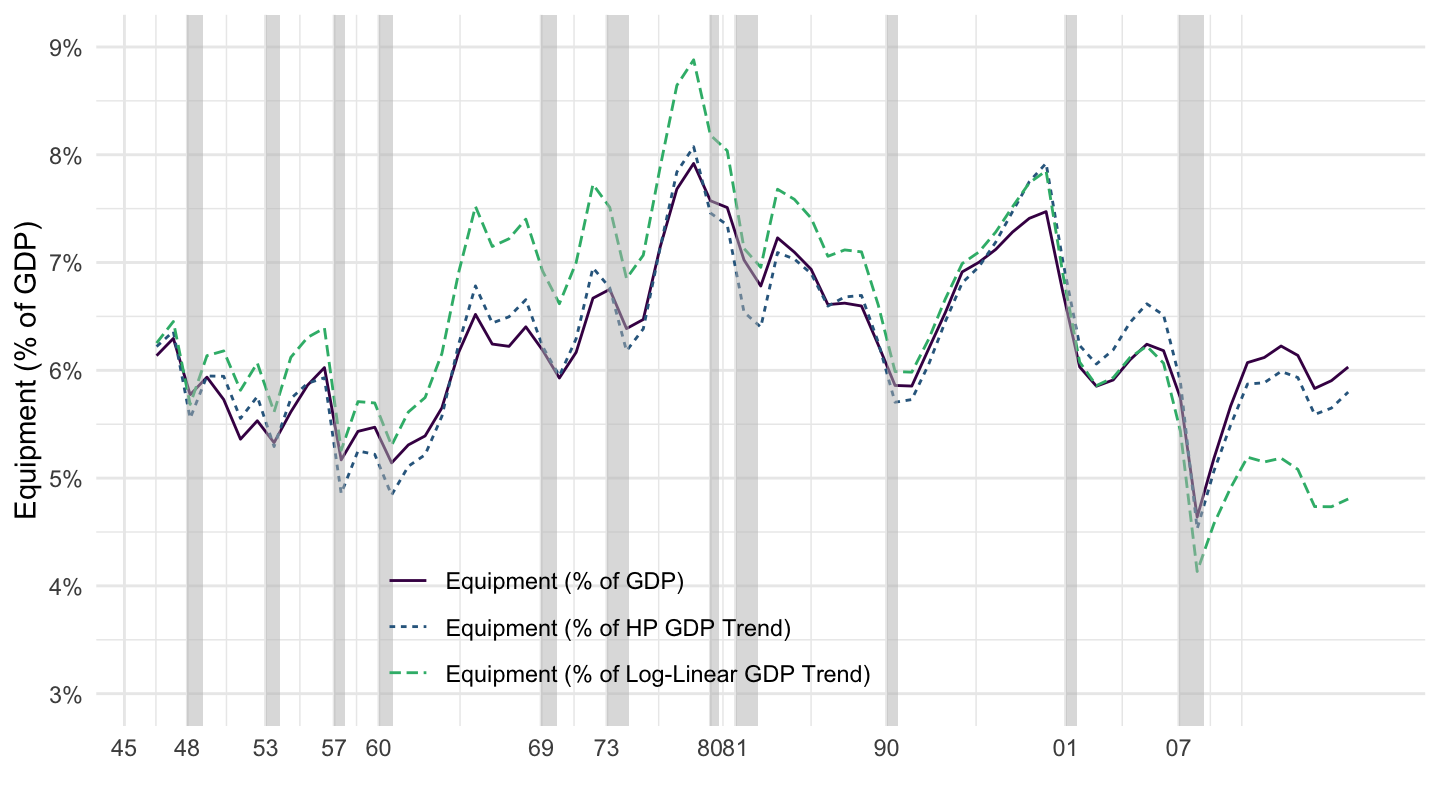
Figure 1.19: Equipment.
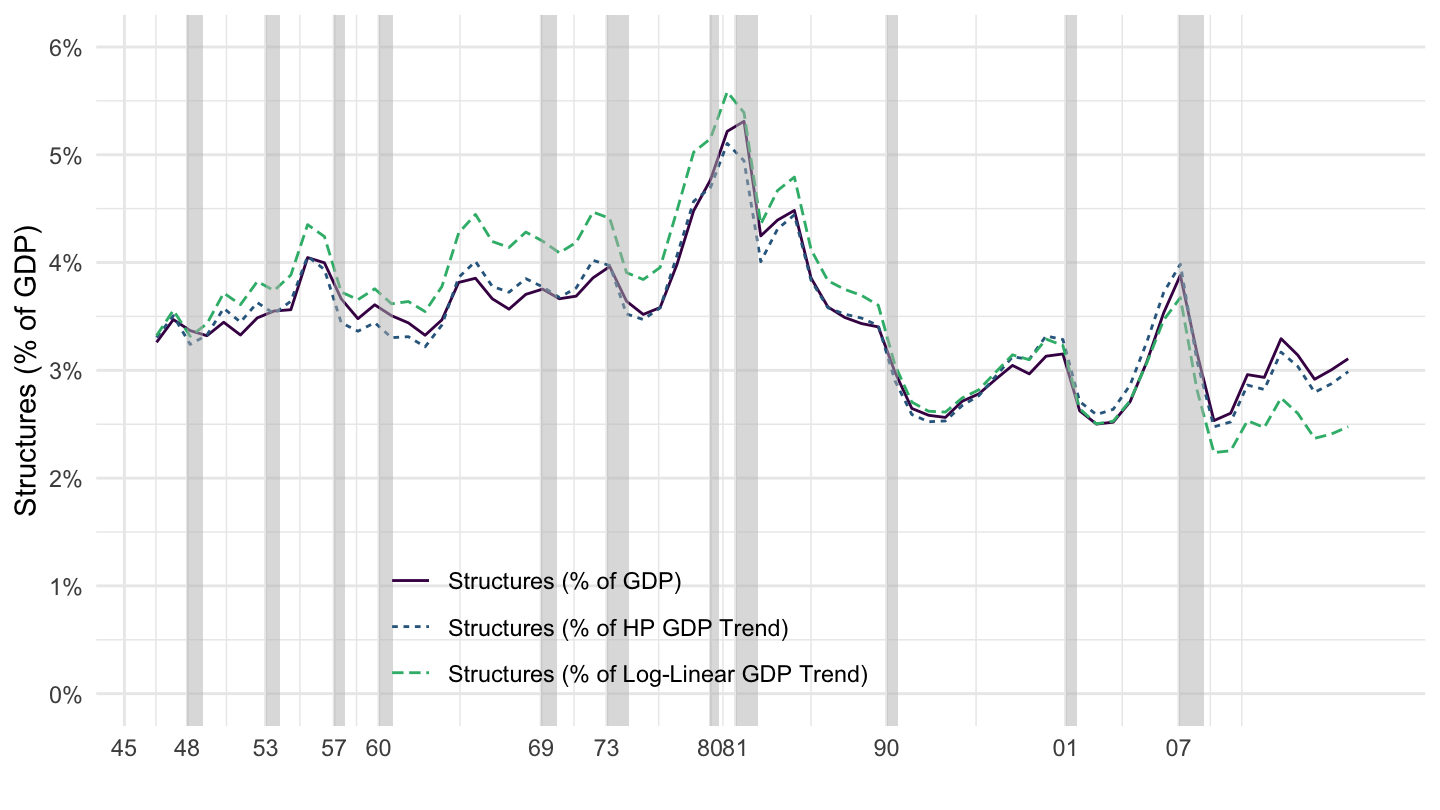
Figure 1.20: Structures.
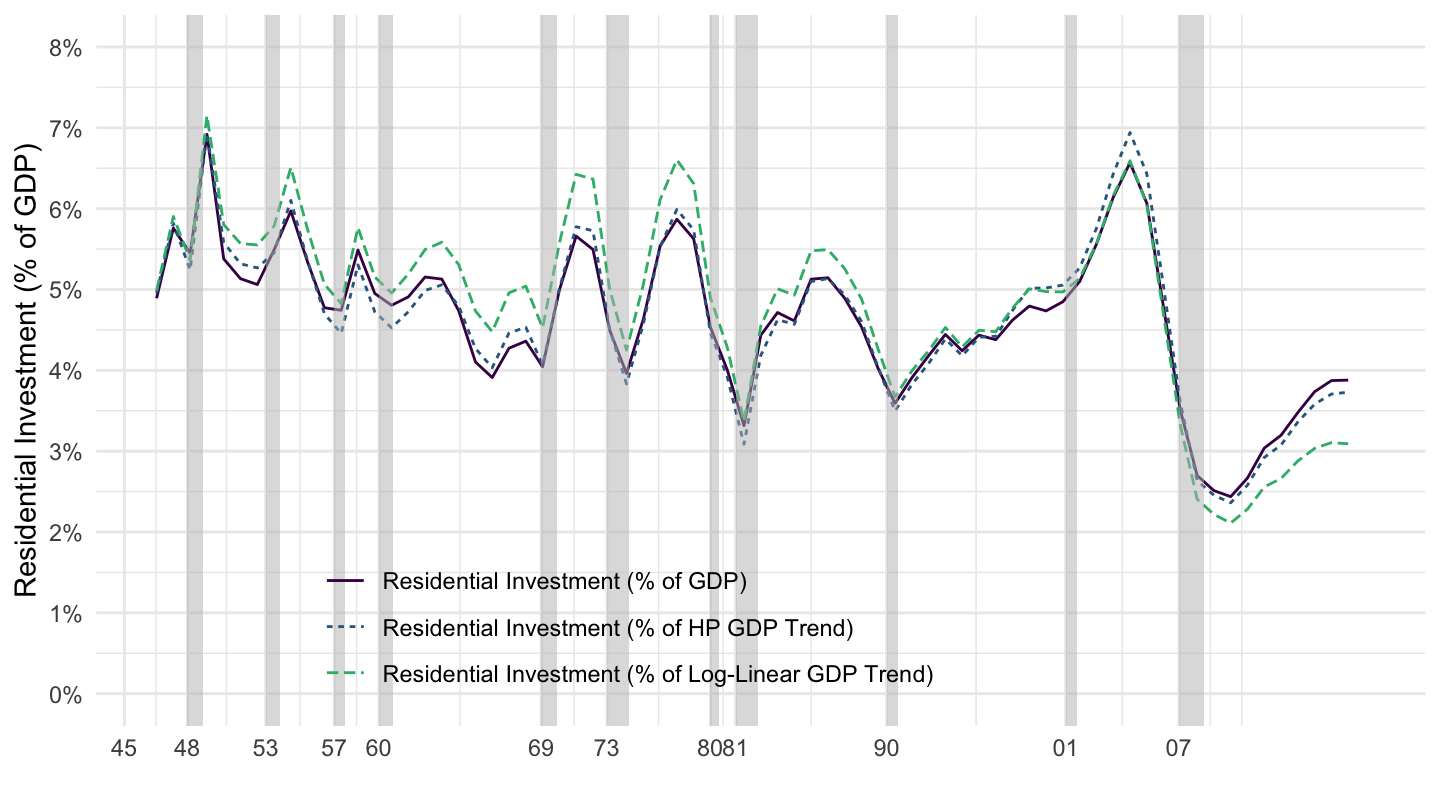
Figure 1.21: Residential Investment.
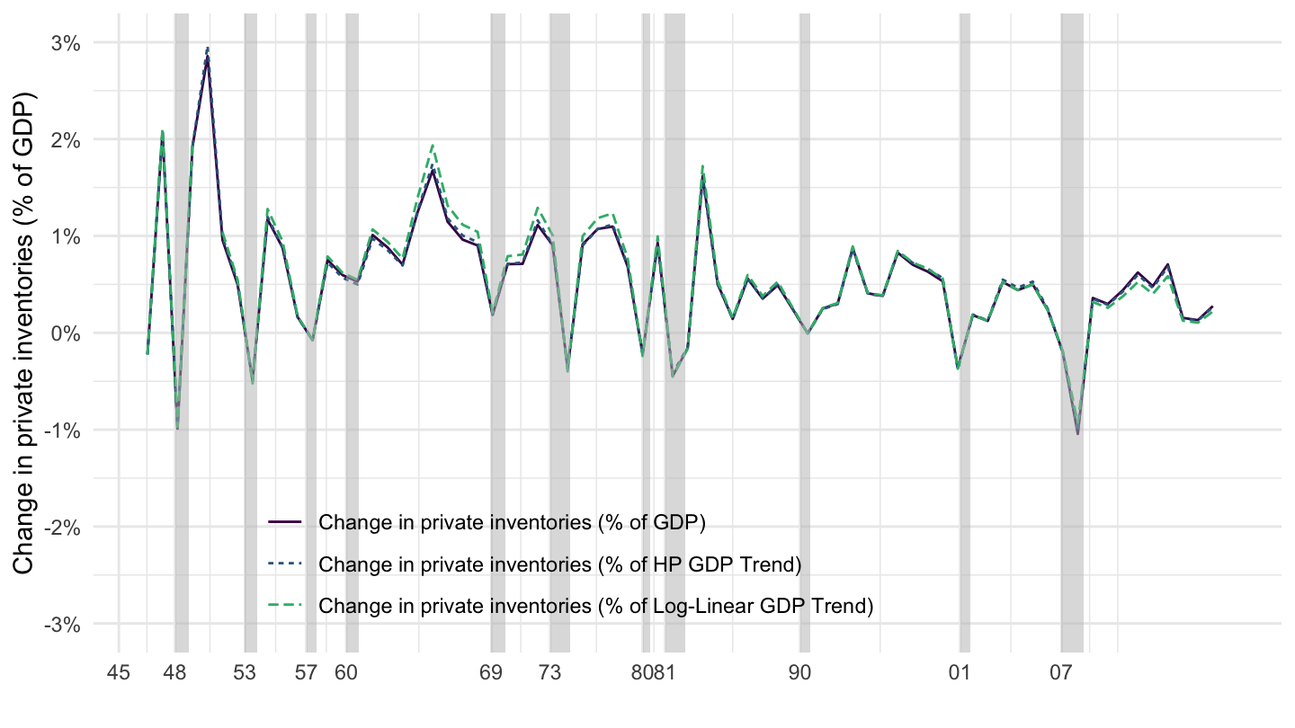
Figure 1.22: Change in Private Inventories.
1.6 Product Approach: Government Purchases
Government purchases are composed of purchases of goods by the government plus the compensation of government employees. Overall, they comprise about approximately 20% of GDP, as can be seen on Figure 1.23. Note however that they do not include transfers from the government of interest payments on government debt.
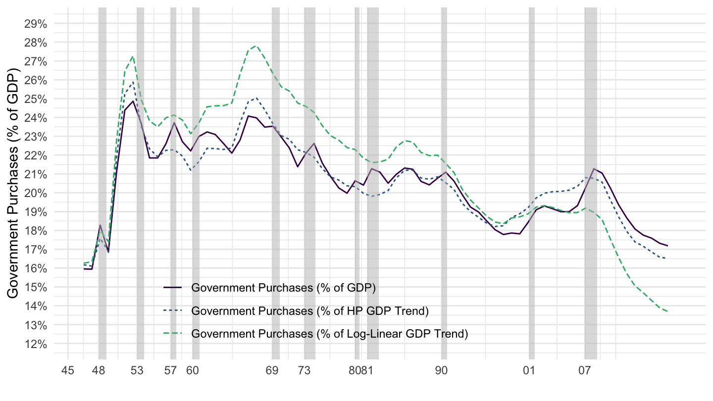
Figure 1.23: Government Purchases.
1.7 Product Approach: Net Exports
Net exports of goods and services are approximately -2 to -6 % of GDP, at least in the modern period (and in the U.S.), as you can see on Figure 1.24.
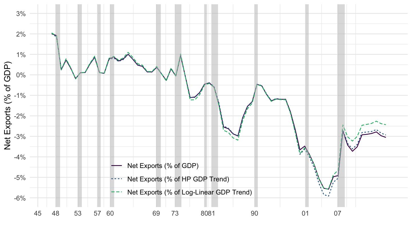
Figure 1.24: Net Exports.
1.8 The Income Approach to GDP
Cobb-Douglas Production function. In order to organize our thinking, let’s write out a Cobb-Douglas production function, defined as: \[Y_t = A_t K_t^{\alpha} L_t^{1-\alpha},\] where \(\alpha\) is a number between \(0\) and \(1\). We will see later that this \(\alpha\) is related to the share of capital versus labor in value added. In practice, you should think of \(\alpha\) as close to \(1/3\). Again, we shall explain why at the end of this lecture.
To proceed further, it is useful to think of a firm which would choose the amount of labor it uses \(L_t\) as well as the amount of capital it uses \(K_t\) in order to maximize its profits:4 \[\max_{K_t, L_t} \quad A_t K_t^{\alpha} L_t^{1-\alpha} - R_t K_t - w_t L_t,\]
In this expression, \(R_t\) is the rental rate of capital, also called the gross return to capital. This represents how much it costs to rent one unit of capital. This cost actually has two components:
It includes a conventional interest rate \(r_t\), which is the cost of borrowing money to invest in capital. You should think of this as the real interest rate which is charged by a bank to borrow money.
It also includes a depreciation rate \(\delta\), which accounts for the wear and tear of the capital stock, implying that its value drops over time. If capital is bought, then the resale price for each unit of capital is lower by a fraction \(\delta\), which is a cost to the investor. If capital is rented, then capital needs to be given back to the owner in its original state.
We have that the rental rate or gross return is equal to the net return plus the depreciation rate: \[\boxed{R_t = r_t + \delta}.\] From Econ 11, it should be clear that a way to solve this problem is to set the derivative of the profit function equal to \(0\) with respect to \(K_t\) and \(L_t\):
- Differentiating with respect to \(K_t\) implies: \[ \begin{aligned} \alpha A_t K_t^{\alpha-1} L_t^{1-\alpha} - R_t = 0 \quad \Rightarrow \quad \boxed{R_t = \alpha A_t K_t^{\alpha-1} L_t^{1-\alpha}}. \end{aligned} \]
- Differentiating with respect to \(L_t\) implies: \[(1-\alpha) A_t K_t^{\alpha} L_t^{-\alpha} - w_t = 0 \quad \Rightarrow \quad \boxed{w_t = (1-\alpha) A_t K_t^{\alpha} L_t^{-\alpha}}.\]
Note that an alternative, and more direct way to get at that same result, would be to use Econ 11 directly, and write that the marginal products have to be equal to prices:
- The rental rate of capital \(R_t\) is the marginal product of capital. The marginal product of capital is how much more output is obtained when the capital stock is increased by one unit, which is just the derivative of output with respect to capital \(\partial Y_t / \partial K_t\): \[ \begin{aligned} R_t&=\frac{\partial Y_t}{\partial K_t}\\ &= \frac{\partial \left(A_t K_t^{\alpha} L_t^{1-\alpha}\right)}{\partial K_t}\\ R_t &= \alpha A_t K_t^{\alpha-1} L_t^{1-\alpha} \end{aligned} \]
- The wage \(w_t\) is the marginal product of labor. The marginal product of labor is how much more output is obtained when the quantity of labor is increased by one unit, which is just the derivative of output with respect to labor \(\partial Y_t / \partial L_t\): \[ \begin{aligned} w_t &=\frac{\partial Y_t}{\partial L_t}\\ &= \frac{\partial \left(A_t K_t^{\alpha} L_t^{1-\alpha}\right)}{\partial L_t}\\ w_t &= (1-\alpha) A_t K_t^{\alpha} L_t^{-\alpha} \end{aligned} \]
The total capital income \(R_t K_t\) is a fraction \(\alpha\) of output \(Y_t\): \[ \begin{aligned} R_t K_t &= \alpha A_t K_t^{\alpha-1} L_t^{1-\alpha} \cdot K_t \\ &= \alpha A_t K_t^{\alpha} L_t^{1-\alpha}\\ R_t K_t &= \alpha Y_t. \end{aligned} \] This implies that the share of capital income in output (or equivalently, value added) is: \[\boxed{\frac{R_t K_t}{Y_t}=\alpha}.\]
The total wage bill \(w_t L_t\) is a fraction \(1-\alpha\) of output \(Y_t\): \[ \begin{aligned} w_t L_t &= (1-\alpha) A_t K_t^{\alpha} L_t^{-\alpha} \cdot L_t \\ &= (1-\alpha) A_t K_t^{\alpha} L_t^{1-\alpha}\\ w_t L_t &= (1-\alpha) Y_t \end{aligned} \] The share of labor income in output \(w_t L_t/Y_t\) (or equivalently, value added) is: \[\boxed{\frac{w_t L_t}{Y_t}=1-\alpha}.\]
Note that capital income plus labor income equals total output: \[R_t K_t + w_t L_t = Y_t.\] Another way to say the same thing is that the share of capital income in output and that of labor income in output add up to one: \[\boxed{\frac{R_t K_t}{Y_t} + \frac{w_t L_t}{Y_t}=1}.\]
The Income Side in the Data. In practice, how much goes to the compensation of employees (labor income), and how much goes to the returns to capital (capital income)? The answer is that it goes approximately for 1/3 to capital and for 2/3 to labor. In turn, this implies that we will, in numerical applications of our theories, often assume that: \[\alpha = \frac{1}{3}\] The calculations for these are less straightforward than for computing the share of consumption, investment, as we did above. The reason is that in practice, the division between labor and capital is not as clear cut in the national accounts as one might hope: for example, someone who owns her/his own business reports most of her/his income in the form of capital income, even when a large part of it is actually labor income, so that compensation of employees is (vastly) understated. Figure 1.25 shows which results are obtained using this understated measure. It needs to be adjusted upwards by about 10% of GDP, for the reasons mentioned above.
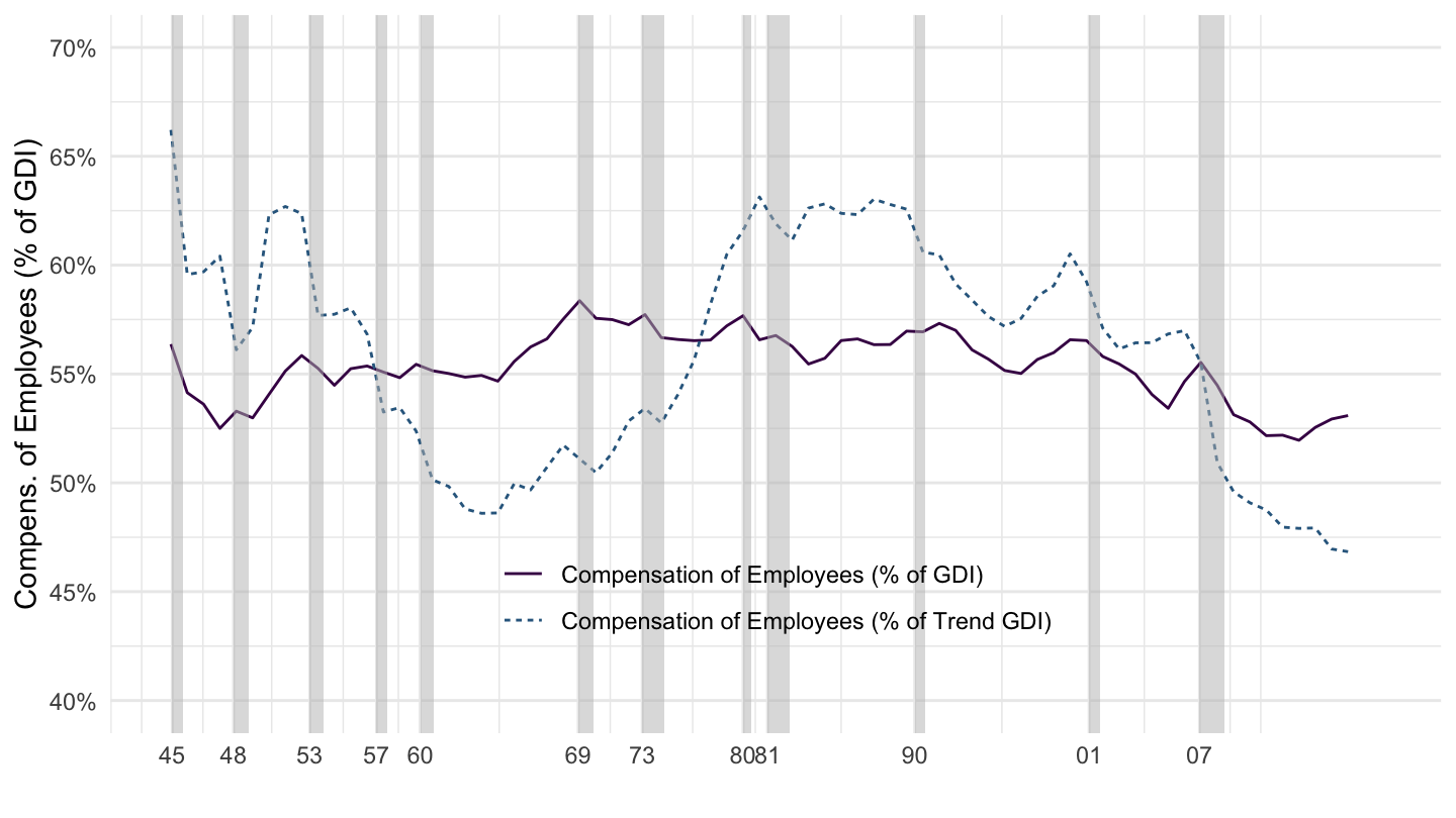
Figure 1.25: Compensation of Employees.
For our purposes, we only need to remember that the share of compensation of employees is approximately 2/3 of value added: \[1-\alpha \approx \frac{2}{3} \quad \Rightarrow \quad \boxed{\alpha \approx \frac{1}{3}}.\]
Therefore, we will very often work with a Cobb-Douglas production function where \(\alpha=1/3\), implying that production is given by: \[Y_t = A_t K_t^{1/3} L_t^{2/3}.\] The next chapters will walk you through the Solow growth model, where we shall make heavy use of that Cobb-Douglas production function.
In some textbooks (as well as in earlier versions of these lecture notes), imports are denoted by \(IM\) instead of \(M\).↩
You may be asking yourself what this firm is. We are looking at aggregates here, and there sure isn’t just one firm in the economy. However, if all firms were identical, because of constant return to scale, the “representative” firm aggregating the decisions of all individual firms would seem to be solving that problem.↩