6 The Labor Market and Unemployment
Link to slides / Link to handouts
Understanding why unemployment occurs is probably one of the most important question for macroeconomics. To quote Paul Samuelson in the First Edition of his Principles of Economics, in 1948:
When, and if, the next great depression comes along, anyone of us may be completely unemployed - without income or prospects. Or if not totally unemployed, only partially employed at reduced hours and pay in an uninteresting dead-end job, without hope of advancement or assurance of keeping even what little we have. There is no vaccination or advance immunity from this modern-day plague. It is no respecter of class or rank. Neither veteran’s preference nor go-getter pep talks nor advanced degrees can guarantee a job when whole factories are shutting down and when every industry is contracting production and employment.
From a purely selfish point of view, then, it is desirable to gain understanding of the first problem of modern economics: the causes on the one hand of unemployment, overcapacity, and depression; and on the other of prosperity, full employment, and high standards of living. But no less important is the fact - clearly to be read from the history of the twentieth century — that the political health of a democracy is tied up in a crucial way with the successful maintenance of stable high employment and living opportunities. It is not too much to say that the widespread creation of dictatorships and the resulting World War II stemmed in no small measure from the world’s failure to meet this basic economic problem adequately.
This question probably is also the most debated one. Market economies go through periods where many people are “unemployed”, in the sense that they would like to work but do not find available employment. Figure 6.1 plots the time series of the U.S. unemployment rate. NBER recessions are shaded in grey. It can be observed that U.S. recessions correspond to substantial rises in the unemployment rate.
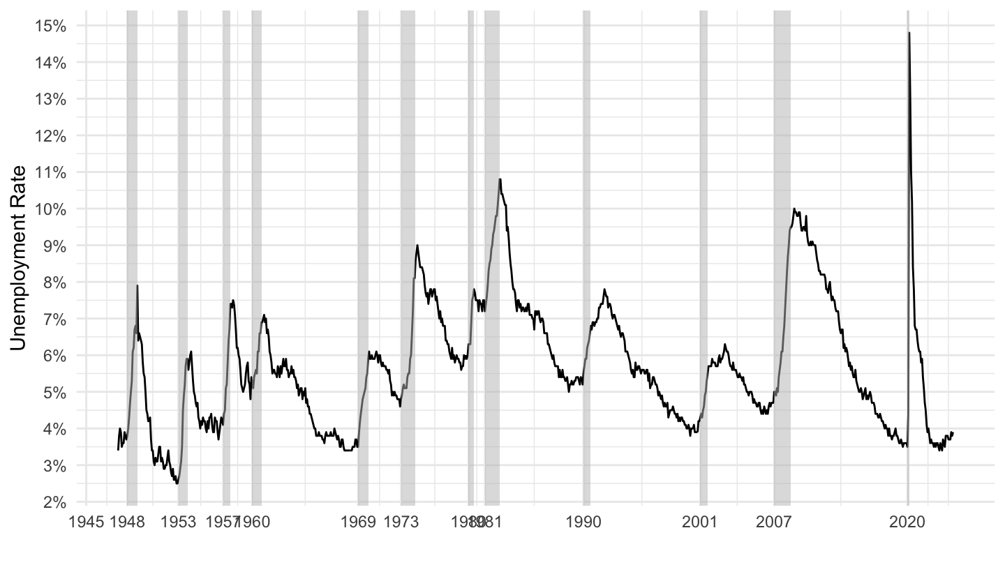
Figure 6.1: U.S. Unemployment Rate (Source: FRED).

Figure 6.2: U.S. Labor Force Participation (Source: Bureau of Labor Statistics).

Figure 6.3: U.S. Labor Force Participation (Source: Bureau of Labor Statistics).
This lecture goes over three different models of the labor market, each of which has a different explanation for the phenomenon of unemployment:
- the Neoclassical model in section 6.1,
- the Keynesian model in section 6.2,
- the Bathtub model in section 6.3.
In this lecture, we examine each of them in turn.
6.1 The Neoclassical Model
Neoclassical economic theory is fundamentally based on the laws of supply and demand. In this theory, labor is treated as another good, which enters negatively in the utility function of workers because people would rather not work (therefore, labor is a “bad” rather than a “good”). Labor is also a useful input into production, which allows firms to sell consumption goods to workers. In the neoclassical theory, the real wage is determined at the intersection of supply and demand.
Labor Demand. Firms hire labor at price \(w\), and sell the consumption good a price \(p\). Assume that the production function is decreasing returns to scale with respect to labor (think for example, that the quantity of capital is fixed): \[y = f(l).\] Then, firms maximize their profits, and therefore solve: \[\max_l \quad pf(l) - wl.\]
Labor Supply. Neoclassical theory of labor supply starts from a static problem of a consumer-worker choosing how much to work, and how much to consume. For example, assume that utility is strictly increasing in consumption, and strictly decreasing in the amount of labor supplied: \[U(c, l)=u(c)-v(l),\] so that the consumer-worker likes to consume, but does not like working. If the price of consumption is \(p\), and assuming a static problem, the budget constraint of a worker/consumer is given by: \[pc = wl.\] You may think of \(w\) as the hourly wage, for example $15/hour. Then \(l\) would be expressed in terms of the number of hours.23
Solution The problem of labor demand shown above leads to the following first-order condition: \[pf'(l)-w = 0 \quad \Rightarrow \quad f'(l)=\frac{w}{p}.\] This equation has a straightforward interpretation: at the optimum, the marginal product of labor - that is, how much is gained from using one more unit of labor in production \(f'(l)\) - needs to be equal to how much that additional unit of labor costs to the firm, the real wage \(w/p\). J.M. Keynes calls it the first fundamental postulate of classical economics in Chapter 2 of the General Theory.
On the other hand, the problem of the consumer consists in maximizing utility under his budget constraint: \[ \begin{aligned} \max_{c,l}& \quad u(c)-v(l),\\ &\text{s.t.}\quad p \cdot c = w \cdot l. \end{aligned} \]
Again, similarly to the consumption optimization problem of lecture 2, you may solve this optimization in four different ways:
You may compute the ratio of marginal utilities (the marginal rate of substitution between consumption and labor) and state that it is equal to minus the real wage (because labor slackens the intertemporal budget constraint, and it appears on the right hand-side of the equal sign): \[\frac{\partial U / \partial l}{\partial U / \partial c} = -\frac{w}{p} \quad\Rightarrow\quad \boxed{\frac{v'(l)}{u'(c)}=\frac{w}{p}}\]
You may apply the following intuitive economic argument. The marginal disutility from supplying one more unit of labor is \(v'(l)\), for a worker already supplying \(l\) units of them. The marginal utility which is gained from doing so is given by the number of additional units of consumption one gets out of it, given by the real wage \(w/p\), and by how much I value each one of these additional utilities of consumption is valued, given by marginal utility \(u'(c)\). The total gain in utility from consumption is the unit value \(u'(c)\) times the number of units \(w/p\), which gives the result: \[v'(l)=\frac{w}{p}u'(c)\quad \Rightarrow \quad \boxed{\frac{v'(l)}{u'(c)}=\frac{w}{p}.}\] J.M. Keynes, who did not write one equation in his General Theory, calls this the second postulate of the classical economics, in Chapter 2: “The utility of the wage when a given volume of labour is employed is equal to the marginal disutility of that amount of employment.”
- You may substitute out \(l\) from the budget constraint, and optimize over the choice of consumption: \[\max_c \quad u(c)-v\left(\frac{p}{w} c\right).\] This implies: \[u'(c)-\frac{p}{w}v'(l)=0 \quad \Rightarrow \quad \frac{v'(l)}{u'(c)}=\frac{w}{p}.\]
You may substitute out \(c\) from the budget constraint, and optimize over the choice of labor: \[\max_l \quad u\left(\frac{w}{p}l\right)-v(l).\] This implies: \[\frac{w}{l}u'(c)-v'(l)=0 \quad \Rightarrow \quad \boxed{\frac{v'(l)}{u'(c)}=\frac{w}{p}}.\]
A Simple Example. Assume a Cobb-Douglas production function for \(f(l)\), such that: \[f(l)=A l^{1-\alpha}.\] In the background, you can really think that the capital stock is exogenous and taken to be equal to \(K=1\), which would lead to this production function exactly.
Let us also assume linear utility for consumption (that is, people enjoy increasing utility equally, regardless of whether it is coming from the first dollar or the last one - this assumption is not realistic and is really made for simplicity), as well as a power function of disutility for work: \[u(c)=c, \quad v(l)=B\frac{l^{1+\epsilon}}{1+\epsilon}\] so that: \[U(c, l)=c-B\frac{l^{1+\epsilon}}{1+\epsilon}.\]
Results. Using the above functional forms for \(u(.)\) and \(v(.)\) allows to write: \[v'(l)=Bl^{\epsilon}, \quad u'(c)=1, \quad \Rightarrow \quad Bl^{\epsilon} = \frac{w}{p}.\] Labor supply \(L^{s}(.)\) as a function of the real wage \(w/p\) is thus given by: \[l =\frac{1}{B^{1/\epsilon}} \left(\frac{w}{p}\right)^{1/\epsilon} \equiv L^s\left(\frac{w}{p}\right).\] Moreover, using the above functional form for \(f(.)\) allows to write: \[f'(l) =A(1-\alpha)l^{-\alpha} \quad \Rightarrow \quad A(1-\alpha)l^{-\alpha}=\frac{w}{p}.\] Therefore, labor demand \(L^d(.)\) is given as a function of the real wage \(w/p\) by: \[l=A^{1/\alpha}(1-\alpha)^{1/\alpha}\left(\frac{w}{p}\right)^{-1/\alpha}\equiv L^d\left(\frac{w}{p}\right).\] To sum up, the neoclassical labor market model is composed of the following labor supply and labor demand equations: \[ \begin{aligned} L^d\left(\frac{w}{p}\right) &= A^{1/\alpha}(1-\alpha)^{1/\alpha}\left(\frac{w}{p}\right)^{-1/\alpha},\\ L^s\left(\frac{w}{p}\right) &= \frac{1}{B^{1/\epsilon}} \left(\frac{w}{p}\right)^{1/\epsilon}. \end{aligned} \] Market clearing implies that labor supply equals labor demand: \[ \begin{aligned} &L^d\left(\frac{w}{p}\right) = L^s\left(\frac{w}{p}\right) \\ &\quad \Rightarrow \quad A^{1/\alpha}(1-\alpha)^{1/\alpha}\left(\frac{w}{p}\right)^{-1/\alpha} = \frac{1}{B^{1/\epsilon}} \left(\frac{w}{p}\right)^{1/\epsilon} \\ &\quad \Rightarrow \quad \left(\frac{w}{p}\right)^{\frac{1}{\alpha} +\frac{1}{\epsilon}}= (1-\alpha)^{1/\alpha}A^{1/\alpha} B^{1/\epsilon}\\ & \quad \Rightarrow \quad \frac{w}{p} = (1-\alpha)^{\frac{\epsilon}{\alpha+\epsilon}}A^{\frac{\epsilon}{\alpha+\epsilon}} B^{\frac{\alpha}{\alpha+\epsilon}}. \end{aligned} \]
We may use either labor supply or labor demand in order to express the equilibrium quantity of labor \(l\). For example, let us use labor demand (as an exercise, you may check that using labor supply instead leads to the same expression): \[ \begin{aligned} l&=\frac{1}{B^{1/\epsilon}} \left(\frac{w}{p}\right)^{1/\epsilon}\\ &=\frac{1}{B^{1/\epsilon}} (1-\alpha)^{\frac{1}{\alpha+\epsilon}}A^{\frac{1}{\alpha+\epsilon}} B^{\frac{\alpha}{\epsilon(\alpha+\epsilon)}}\\ &= (1-\alpha)^{\frac{1}{\alpha+\epsilon}}A^{\frac{1}{\alpha+\epsilon}} B^{\frac{\alpha}{\epsilon(\alpha+\epsilon)}-\frac{1}{\epsilon}}\\ l&= (1-\alpha)^{\frac{1}{\alpha+\epsilon}}A^{\frac{1}{\alpha+\epsilon}} B^{-\frac{1}{\alpha+\epsilon}} \end{aligned} \]
An Example: A Shock to Labor Demand. Assume that firms all of a sudden become less productive: that is, \(A\) declines. This corresponds to a shift in the labor demand curve to the left (because \(A\) appears in the labor demand curve). As a consequence, the graph shows that clearly the equilibrium number of hours declines, and the real wage falls. The algebra above can also be used in order to show that a reduction in \(A\) both leads to a fall in the number of hours as well as to a fall in the real wage. Note that in the neoclassical model, there is nothing that explains why the fall in hours worked goes through the extensive margin (the number of people employed) rather than at the intensive margin (how intensively everyone works). In practice, some countries such as Germany have put in place work sharing programs during the depression, in order to share the reduction in employment equally among workers, rather than proceed to lay-off workers.
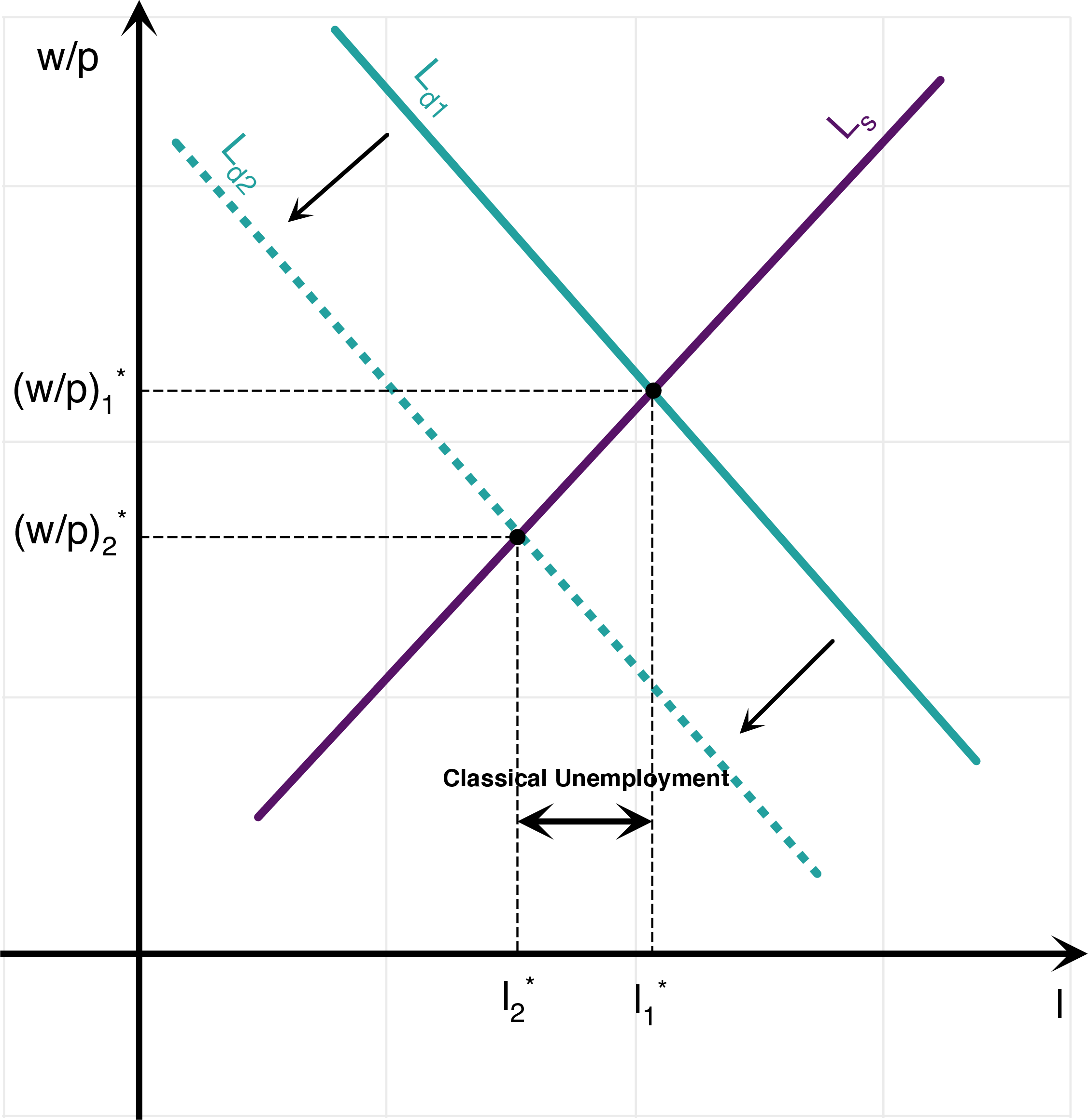
Figure 6.4: Shock to Labor Demand in the Neoclassical Model.
6.2 The “Keynesian” Model
There are two ways in which the neoclassical model above is not satisfying. Empirically, the real wage moves very little during recessions, compared to the increase in unemployment, an observation which is usually viewed as inconsistent with the neoclassical model. Moreover, and probably more importantly, the neoclassical model assumes that all unemployment is voluntary. In contrast, intuitively, the level of employment appears “too low” during recessions, in the sense that many people seem to be looking for work, but do not find one.
One potential explanation might be that wages are sticky (at least downwards). In that case, the graph shows that following a shock to labor demand, labor demand might be lower than labor supply: there is involuntary unemployment, in the sense that some workers want to work more than they do at the prevailing market wage. Workers are said to be “off their labor supply curve”, because it is the level of the demand for labor that determines the employment level.
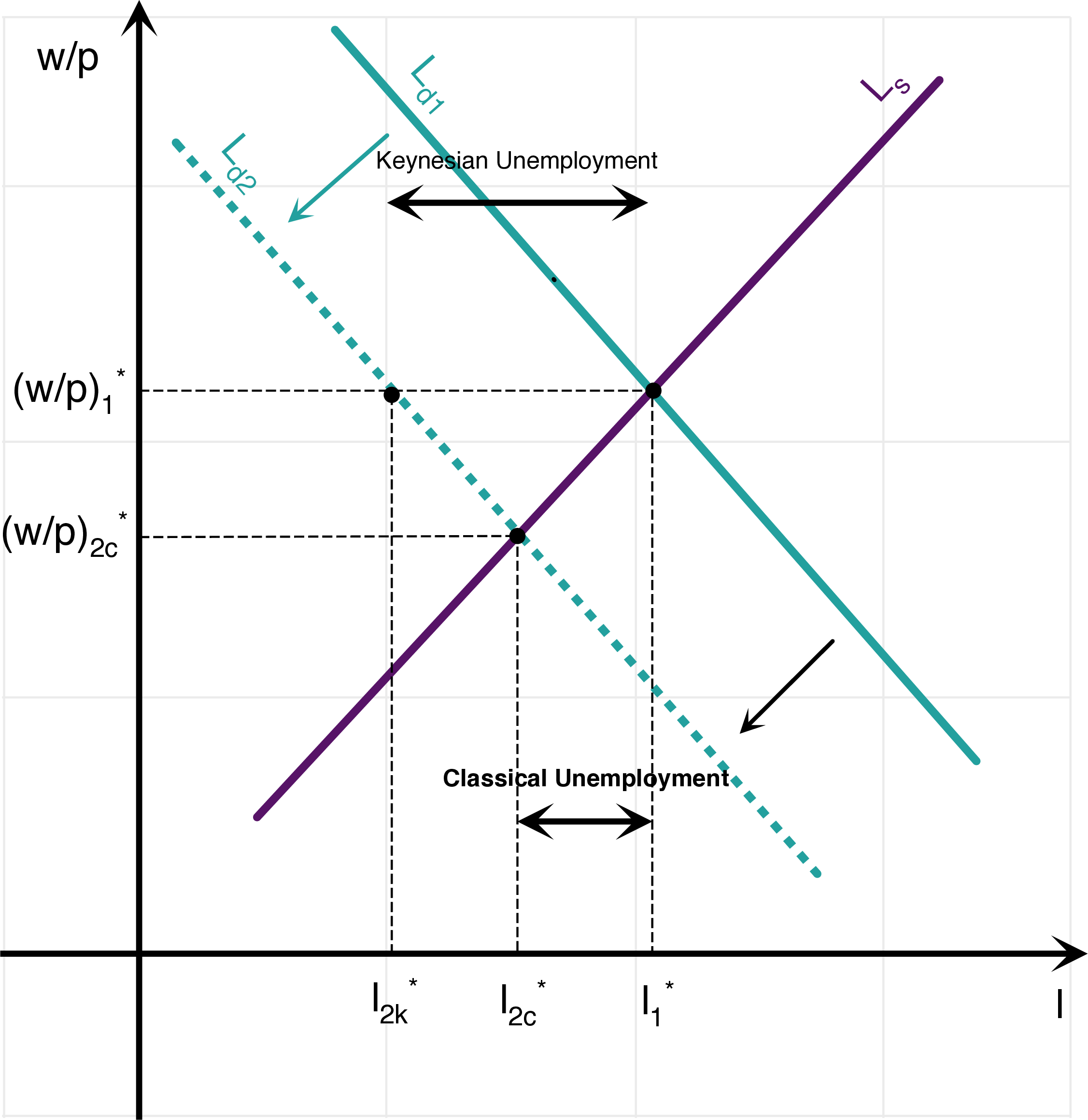
Figure 6.5: Shock to Labor Demand in the Neoclassical and Keynesian Models.
The graph shows clearly that “Keynesian” unemployment is larger than Classical Unemployment: employment falls by more than if wages were flexible.
Finally, I use quotes for “Keynesian” because although John Maynard Keynes mentioned sticky wages in The General Theory of Employment, Interest and Money as a potential cause for unemployment, his thought was much more complex, and he did not see a reduction in real wages as a cure for unemployment. Although rigid wages have become synonymous with Keynes’ thought in many textbooks, you should keep in mind that John Maynard Keynes’ thought was much more complex than this, and that J.M. Keynes actually was not in favor of a reduction in wages to cure unemployment problems (you can see for yourself directly in The General Theory). If you want to know more, The Economist has a great briefing on the natural rate of unemployment - however, we will not investigate these notions any further, so you are not responsible for the content of this article.
6.3 The Bathtub Model
A final view of unemployment consists in a mechanical, almost statistical model of the labor market, called the “bathtub” model of unemployment. This view recognizes that the labor market involves constant churning, which implies that there always are some workers who are in between jobs. It is called the bathtub model of unemployment because in some ways, the unemployment rate is quite similar to the height of the water in a bathtub.
Model. In the bathtub model of unemployment, there is a number \(L\) of people in the labor force. Jobs separate at a rate \(s\), often called the job separation rate, and the rate at which unemployed people find new jobs is \(f\), the job finding rate. For example, assuming that in a typical month, 20% of the unemployed find new jobs, then \(f=20\)%. If, on the other hand, 1% of the employed lose their jobs, then \(s=1\)%. Finally, the number of people unemployed is denoted by \(U_{t}\) and the number of people employed as \(E_{t}\). The law of motion for the unemployment population is given by: \[\Delta U_{t+1}=sE_{t}-fU_{t}.\]
Solution. Using the fact that people are either employed or unemployed: \[E_{t}+U_{t}=L,\] and plugging in the law of motion for \(U_t\): \[ \begin{aligned} \Delta U_{t+1}&=U_{t+1}-U_t=s\left(L-U_t\right)-fU_t\\ & \Rightarrow \quad U_{t+1}=(1-s-f)U_t+sL. \end{aligned} \] In the long run, we have that, the number of unemployed people \(U^{*}\) satisfies the following equation: \[U_{t+1}=U_{t}=U^{*}\quad\Rightarrow\quad U^{*}=\frac{sL}{s+f}.\]
The corresponding long run unemployment rate \(u^{*}\), that is the number of unemployed as a function of the total population, is then given by: \[u^{*}=\frac{U^{*}}{L}=\frac{s}{f+s}.\]
Numerical Application. Using the above numerical values, a job separation rate of about \(s=1\)%, as well as a job finding rate of about \(f=20\)%, we get a value for long-run unemployment, sometimes called the natural rate of unemployment, equal to: \[u^{*}=\frac{0.01}{0.2 + 0.01}\approx 4.8\%\].
Transition dynamics. Unlike with the Solow growth model of lecture 1.5, we can do more and ask how the unemployment rate converges to this steady-state level, using the law of motion for unemployment (this was impossible for the Solow growth model because the law of motion for capital was too complex):
\[ \begin{aligned} U_{t+1}&=\left(1-s-f\right)U_{t}+sL\\ & \quad\Rightarrow\quad U_{t+1}-U^{*}=\left(1-s-f\right)\left(U_{t}-U^{*}\right)\\ & \quad\Rightarrow\quad U_{t}=U^{*}+\left(1-s-f\right)^{t}\left(U_{0}-U^{*}\right). \end{aligned} \]
6.4 Data on Job Churning
Data on job churning is collected by the Bureau of Labor Statistics (the Job Opening and Labor Turnover Survey, also known as JOLTS). You may in particular view the latest data on Job openings, Hires levels, Total separations, Quits, Layoffs and discharges.
The evolution of job openings and hire levels on the one hand, and total separations, quits, layoffs and discharges are plotted on the two figures below.
This data shows that there are many ways in which the bathtub model of unemployment is an oversimplification. The rates of total separations and job finding both fall substantially during recessions. This is because total separations come from two things in the real world: some separations are chosen from workers (quits), some of them are chosen by firms (layoffs). Layoffs are the part of total separations which increase during recessions. Third, the job finding rate is also endogenous, because not all job openings lead to hires.
Increased unemployment during recessions is explained by an increase in layoffs, but more importantly by a decline in job openings.
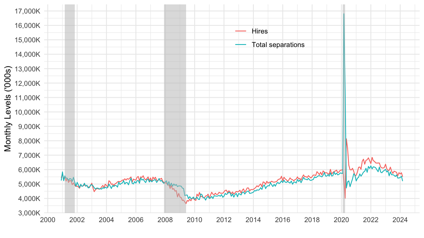
Figure 6.6: Monthly Hires and Separations, in Thousands. Source: BLS-JOLTS.
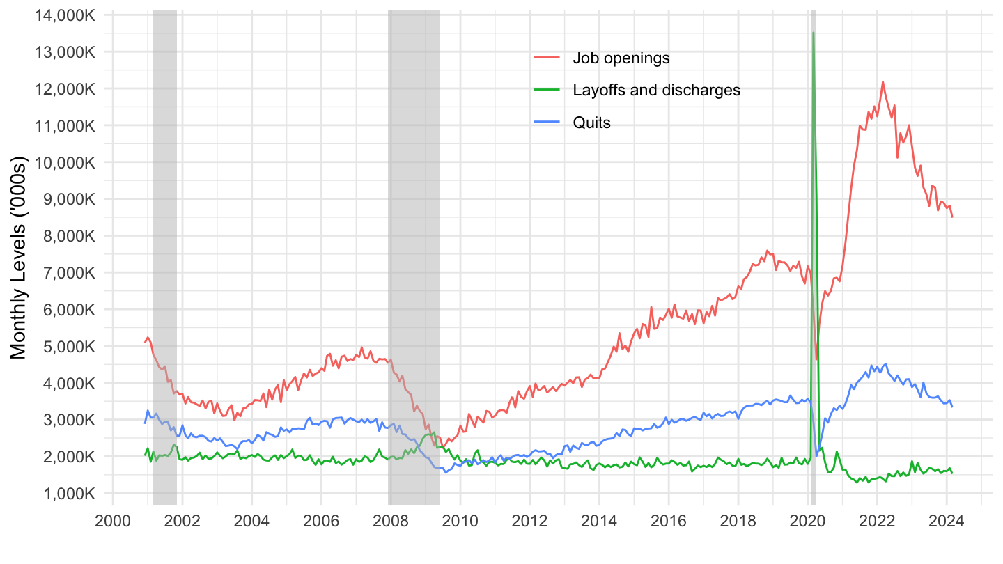
Figure 6.7: Monthly Job Openings, Layoffs and Quits, in Thousands. Source: BLS-JOLTS.
Warning: Labor Supply and Labor Demand are sometimes being mixed up. In the language of microeconomics, workers supply labor, and firms demand labor. What workers do demand is jobs, or job vacancies, which are supplied by firms.↩