9 Redistributive Policies
Link to slides / Link to handouts
9.1 Redistribution according to Neoclassical Economics
Before we look at redistribution in the Keynesian model, we first need to remind ourselves of how to think about redistribution in the supply-side, neoclassical model. In such a model, taxation is always bad because it distorts agents’ incentives to work.
We go back to the labor market model of lecture 6, and study redistribution. Denoting the (hourly) wage by \(w\), the price of consumption by \(p\), and the number of hours (per year) by \(l\), assuming that moreover \(\alpha=0\) so that returns to labor are constant: \[U(c, l)=c-B\frac{l^{1+\epsilon}}{1+\epsilon}, \qquad f(l)=Al^{1-\alpha} = A l.\]
We further assume that the tax and transfer system is such that \(\tau\) is the marginal tax rate, and \(c_0\) is a real subsistence level of income given by the government: \[pc = (1-\tau)wl + p c_0\].
Labor Demand. We first derive labor demand, which corresponds to the firm side. The firm’s problem is to maximize: \[\max_l \quad p\cdot f(l)-w\cdot l.\]
Given that \(f(l)=A\cdot l\), the firm equivalently maximizes: \[\max_l \quad p \cdot A\cdot l-w\cdot l.\]
One way to get the result is, as usual, to take the first-order condition to this problem:25 \[\frac{w}{p}=A.\]
As a consequence: \[p \cdot A=w \quad \Rightarrow \quad \boxed{\frac{w}{p}=A}.\]
The labor demand curve is said to be infinitely elastic.26
In logs, this implies the following horizontal labor demand curve: \[\log\left(\frac{w}{p}\right)=\log A.\]
Labor Supply. Writing that \(c=c_0+(1-\tau)\cdot (w/p) \cdot l\) and plugging the value of \(c\) into the worker’s optimization problem: \[\max_l \quad c_0 +(1-\tau)\frac{w}{p}l -B\frac{l^{1+\epsilon}}{1+\epsilon}.\]
The first-order condition (which we can take here as long as \(\epsilon>0\)) implies: \[(1-\tau) \cdot \frac{w}{p} = B\cdot l^{\epsilon} \quad \Rightarrow \quad \boxed{l = \frac{(1-\tau)^{1/\epsilon}}{B^{1/\epsilon}}\left(\frac{w}{p}\right)^{1/\epsilon}}.\]
In logs, this implies the following labor demand curve: \[\log\left(\frac{w}{p}\right)=\log B-\log (1-\tau)+\epsilon \cdot \log l.\]
\(1/\epsilon\) is the labor supply elasticity: it’s saying by how much labor supply increases in percentage terms when the real wage increases by 1%. Mathematically: \[\frac{d\log l}{d\log(w/p)}=\frac{1}{\epsilon}\]
Putting the two together. The number of hours worked is given by replacing out the real wage \(w/p\) from the labor demand equation to the labor supply equation, so that: \[\boxed{l = (1-\tau)^{1/\epsilon}\frac{A^{1/\epsilon}}{B^{1/\epsilon}}}.\]
Real pre-tax income is when simply given by the real wage times the number of hours. Since the real wage is simply \(A\), we get: \[y = \frac{w}{p} \cdot l = A\cdot(1-\tau)^{1/\epsilon}\frac{A^{1/\epsilon}}{B^{1/\epsilon}}.\]
Finally: \[\boxed{y = (1-\tau)^{1/\epsilon}\frac{A^{1/\epsilon+1}}{B^{1/\epsilon}}}.\]
The revenue which the government gets here is given by \(\tau y\): \[\tau \cdot y = \tau (1-\tau)^{1/\epsilon}\frac{A^{1/\epsilon+1}}{B^{1/\epsilon}}\]
Laffer curve. This expression shows that there are two opposing effects of taxation on tax revenues. On the one hand, there is a positive effect (a direct effect): when \(\tau\) is higher, there are more government revenues. On the other hand, more taxes lower GDP because they reduce the incentives to work (the indirect effect). Defining a constant: \[C \equiv \frac{A^{1/\epsilon+1}}{B^{1/\epsilon}},\] implies that tax revenues are proportional to \(\tau (1-\tau)\): \[\tau \cdot y = C \cdot \tau (1-\tau)^{1/\epsilon}\]
The curve which represents total tax revenues as a function of the rate of taxation is called the Laffer curve, named after Arthur Laffer, a supply-side economist. For \(\tau = 0\%\), no revenue is raised, but for \(\tau = 100\%\), no revenue is raised either because no one wants to work with a share of take-own pay equal to zero. For example, for \(\epsilon=1\), we get a parabola for tax revenues as a function of the tax rate, which has a maximum for \(\tau=1/2\). For any \(\epsilon\), we may compute the revenue maximizing tax rate, which is given by: \[\max_\tau \quad \tau (1-\tau)^{1/\epsilon}.\]
This is maximized for a value of \(\tau\) such that the first derivative is zero: \[(1-\tau)^{1/\epsilon}-\frac{\tau}{\epsilon} (1-\tau)^{1/\epsilon-1}=0.\]
This implies: \[\frac{\tau}{1-\tau}=\epsilon \quad \Rightarrow \quad \tau = \epsilon - \epsilon \tau \quad \Rightarrow \quad \tau = \frac{\epsilon}{\epsilon+1} = \dfrac{1}{1+\dfrac{1}{\epsilon}}.\]
The higher the labor supply elasticity \(1/\epsilon\) (that is, the more people are responsive to changes in net of tax rates), the lowest the tax rate should be. To the limit, if people work no matter what \(\epsilon = +\infty\), then they can be taxed at a confiscatory rate. If they respond a lot to wages (incentives), then taxes should be very low. As you can guess, the value for the labor supply elasticity is subject to intense controversies. We’ll come back to this when we look at empirical macroeconomics.
Marginal tax rates are more distortive when they are the highest. A second result from the neoclassical theory of labor income taxation is that taxes are most distortive where they are initially the highest. Therefore, according to neoclassical economics, taxes should be cut where marginal tax rates are initially the highest (that is, for the richest people). The logic from that argument comes again from the value for income, when subject to a rate of taxation \(\tau\): \[y = (1-\tau)^{1/\epsilon}\frac{A^{1/\epsilon+1}}{B^{1/\epsilon}}.\]
Taking logs of this expression: \[\log(y) = \frac{1}{\epsilon}\log\left(1-\tau\right)+\left(\frac{1}{\epsilon}+1\right)\log A -\frac{1}{\epsilon} \log B.\]
Therefore, a change in marginal taxes \(\tau\) leads to a change in \(y\) given by: \[\frac{d\log(y)}{d\tau}=\frac{1}{\epsilon}\frac{d \log(1-\tau)}{d \tau}.\]
The derivative of \(\log(1-\tau)\) with respect to \(\tau\) is: \[\frac{d \log(1-\tau)}{d \tau}=-\frac{1}{1-\tau}.\]
Therefore, a change in \(\tau\) leads to a change in \(y\) given by: \[\boxed{\frac{d\log(y)}{d\tau}=-\frac{1}{\epsilon (1-\tau)}}.\]
Therefore, the percentage increase in income following a marginal tax cut for a person is an increasing function of \(\tau\), or what is marginal tax rate initially is. Neoclassical economics therefore has a force which suggests the government should cut taxes where marginal tax rates are initially the highest. In other words, taxes should be cut on the richest people, who typically face the largest marginal tax rates, and whose labor supply is therefore already distorted the most.
In the next section, we shall introduce taxation according to Keynesian economics, which typically leads to opposite conclusions.
9.2 Redistribution and Keynesian Economics
Keynesian economics provides a mechanism through which more redistribution might actually increase output overall, at the same time as it reduces inequality. The idea that the economy suffers from a shortage of aggregate demand coming from increases in inequality has been put forward recently by mainstream academics such as Raghuram Rajan, former chief economist of the IMF, and now governor at the Bank of England, as well as by Robert Reich, US Secretary of Labor from 1993 to 1997.
The idea that the MPC is influenced by the distribution of income and wealth comes back to J.M. Keynes in the General Theory:
Since the end of the nineteenth century significant progress towards the removal of very great disparities of wealth and income has been achieved through the instrument of direct taxation—income tax and surtax and death duties—especially in Great Britain. Many people would wish to see this process carried much further, but they are deterred by two considerations; partly by the fear of making skilful evasions too much worth while and also of diminishing unduly the motive towards risk-taking, but mainly, I think, by the belief that the growth of capital depends upon the strength of the motive towards individual saving and that for a large proportion of this growth we are dependent on the savings of the rich out of their superfluity. Our argument does not affect the first of these considerations. But it may considerably modify our attitude towards the second. For we have seen that, up to the point where full employment prevails, the growth of capital depends not at all on a low propensity to consume but is, on the contrary, held back by it; and only in conditions of full employment is a low propensity to consume conducive to the growth of capital. Moreover, experience suggests that in existing conditions saving by institutions and through sinking funds is more than adequate, and that measures for the redistribution of incomes in a way likely to raise the propensity to consume may prove positively favourable to the growth of capital.
This passage from J.M. Keynes in the General Theory is intuitive: as long as saving propensities are no longer an impediment to capital accumulation, redistributing income or wealth from low to high Marginal Propensity to Consume (MPC) should lead to higher output. According to J.M. Keynes, this is in fact one reason for restricting the increase in inequality:
The State will have to exercise a guiding influence on the propensity to consume partly through its scheme of taxation. (…) Whilst, therefore, the enlargement of the functions of government, involved in the task of adjusting to one another the propensity to consume and the inducement to invest, would seem to a nineteenth-century publicist or to a contemporary American financier to be a terrific encroachment on individualism, I defend it, on the contrary, both as the only practicable means of avoiding the destruction of existing economic forms in their entirety and as the condition of the successful functioning of individual initiative.
Similarly, Paul Samuelson states in Chapter 12 of his Principles of Economics textbook:27
To go from the family-budget patterns to the community schedules, we must make some assumptions about the distribution of income: If a national income of 200 billion dollars were exactly divided equally among 40 million families, then the level of total consumption would be higher than if a large proportion of the families fell far above and far below the average level of $5,000 per family. Why is this? Because giving dollars to rich people with low marginal propensities to consume will result in more saving and less consumption than if the income is divided more equally.
During this lecture, we derive this result using the Keynesian model that was developed in lecture ?? and lecture 8. One appeal of writing the equations is that we are not able to prove these assertions qualitatively, but we are also able to understand how important they are quantitatively. As we go along, we therefore attempt to put some actual numbers on all these arguments, to get a sense of the orders of magnitude. We shall investigate two types of policies:
Income redistribution, from high to low income earners.
Deficit-financed decreases in taxes, on high income earners or low income earners, financed by public debt.
9.3 Assumptions
Consumption and Income. Some minor modifications to the goods market model underlying lecture ?? and lecture 8 are in order, in order to think about stimulus policies in the presence of inequality. Instead of assuming one type of consumer, with the average income \(Y\) and a given Marginal Propensity to Consume (MPC) \(c_{1}\), we shall assume two types of workers. We assume that there are \(N\) workers (for practical purposes, think \(N=150\) million):
A fraction \(\lambda\) of low income earners earns income \(\underline{y}\), pays net taxes \(\underline{t}\), and have an MPC equal to \(\underline{c}_{1}\) such that: \[\underline{c}=\underline{c}_{0}+\underline{c}_{1}(\underline{y}-\underline{t}).\]
A fraction \(1-\lambda\) of high income earners earns income \(\bar{y}\), which is a multiple \(\gamma\) of low income earners’ income, given by: \[\bar{y}=\gamma\underline{y},\] where \(\gamma\) is higher when there is more inequality. They each pay net taxes \(\bar{t}\), and the MPC of the high income earners is \(\bar{c}_{1}\): \[\bar{c}=\bar{c}_{0}+\bar{c}_{1}(\bar{y}-\bar{t})\] Moreover, we assume that high income earners have a lower MPC than low income earners, so that: \[\bar{c}_{1}<\underline{c}_{1}\]
Taxes. We also assume that taxes depend on output, both for low income earners: \[\underline{t}=\underline{t}_{0}+t_1\underline{y}\] as well as for high income earners: \[\bar{t}=\bar{t}_{0}+t_1\bar{y}.\]
Investment. Finally, we assume that investment depends on output: \[I=b_{0}+b_{1}Y\]
9.4 Aggregate Demand
Income. Since there is a fraction \(\lambda\) of low income earners, and the total population is \(N\), the total income \(\underline{Y}\) captured by low income earners \(\underline{Y}\) is: \[\underline{Y} = \lambda N \underline y\] Symmetrically, the total income \(\bar{Y}\) captured by high income earners is: \[\bar{Y}=(1-\lambda)N \bar{y}.\] Total income is given by the sum of \(\underline{Y}\), and \(\bar{Y}\), which allows to express low income earners as a function of total income: \[ \begin{aligned} Y&=\underline{Y} + \bar{Y}\\ &=\lambda N \underline{y}+(1-\lambda) N \bar{y}\\ &=\lambda N \underline{y}+(1-\lambda) N \gamma\underline{y}\\ Y&=\left(\lambda +(1-\lambda)\gamma\right)N\underline{y} \end{aligned} \] This implies that low income earners’ \(\underline{y}\) is given as a function of output per person \(Y/N\) and the parameters of the model by: \[\underline{y}=\frac{1}{\lambda+(1-\lambda)\gamma}\frac{Y}{N}\] As a consequence, high income’ individual \(\bar{y}\) is given as a function of output per person \(Y/N\) and the parameters of the model by: \[\bar{y}=\gamma\underline{y}=\frac{\gamma}{\lambda+(1-\lambda)\gamma}\frac{Y}{N}.\] The share of income captured by low income earners is: \[ \begin{aligned} \frac{\underline{Y}}{Y}&=\frac{\lambda N \underline{y}}{\left(\lambda +(1-\lambda)\gamma\right)N\underline{y}}\\ \frac{\underline{Y}}{Y}&=\frac{\lambda}{\lambda +(1-\lambda)\gamma}. \end{aligned} \] The share of income captured by high income earners is: \[ \begin{aligned} \frac{\bar{Y}}{Y}&=\frac{(1-\lambda) N \bar{y}}{\left(\lambda +(1-\lambda)\gamma\right)N\underline{y}}\\ &=\frac{(1-\lambda)\gamma N \underline{y}}{\left(\lambda +(1-\lambda)\gamma\right)N\underline{y}}\\ \frac{\bar{Y}}{Y}&=\frac{(1-\lambda)\gamma}{\lambda +(1-\lambda)\gamma}. \end{aligned} \]
Numerical Application: Approximate the number of workers in the U.S. to about 150 million: \[N = 150,000,000\] and that GDP is 20 trillion. Therefore, GDP per worker on average is: \[\frac{Y}{N}=\$133,333.33\] Let us divide the population in two groups, the top 10% income share, and the bottom 90% income share, so that: \(\lambda = 0.9\). Since the top 10% get approximately 50% of the income in the U.S. (the exact data is available here), this implies, using the formula above \(\underline{Y}/Y=\lambda/\left(\lambda +(1-\lambda)\gamma\right)\): \[\frac{0.9}{0.9+0.1\cdot \gamma}=0.5 \quad \Rightarrow \quad \gamma = 9.\] This is actually very intuitive: if 90% of the population have the same income as 10% of the population (half of total income), then on average they are 9 times poorer. The average income for someone in the top 10% is then: \[\bar{y}=\gamma\underline{y}=\frac{\gamma}{\lambda+(1-\lambda)\gamma}\frac{Y}{N}=\$666,666.66\] They are: \[(1-\lambda) N = 15,000,000.\] While the average income for someone in the bottom 90% is: \[\underline{y}=\frac{1}{\lambda+(1-\lambda)\gamma}\frac{Y}{N}=\$74,074.07.\] They are: \[\lambda N = 135,000,000.\]
Taxes. Aggregate taxes \(T\) are the sum of taxes paid by the low income earners \(\underline{T}\) and the high income earners \(\bar{T}\): \[ \begin{aligned} T&=\underline{T} + \bar{T}\\ &=\lambda N \underline{t} + (1-\lambda) N \bar{t} \\ &=\lambda N \left(\underline{t}_{0}+t_1\underline{y}\right) + (1-\lambda) N \left(\bar{t}_{0}+t_1\bar{y}\right)\\ &=\left(\lambda N \underline{t}_{0} + (1-\lambda) N \bar{t}_{0}\right) + t_1\left(\lambda N \underline{y} + (1-\lambda)N\bar{y} \right)\\ T&=\left(\underline{T}_{0} + \bar{T}_{0}\right) + t_1 Y \end{aligned} \]
The aggregate baseline level of taxes \(T_0\) is: \[T_{0} \equiv \underline{T}_0 + \bar{T}_0 = \lambda N \underline{t}_0 + (1-\lambda) N \bar{t}_0,\] where baseline level of taxes for low and high income earners is given by: \[\underline{T}_0\equiv\lambda N \underline{t}_0, \qquad \bar{T}_0\equiv(1-\lambda) N \bar{t}_0.\] To conclude, total aggregate taxes are: \[ \begin{aligned} \boxed{T=\left(\underline{T}_{0}+\bar{T}_{0}\right)+t_1 Y}. \end{aligned} \]
Consumption. The challenging part, which differs from the models seen in lecture ?? and lecture 8, is to calculate aggregate consumption, which is composed both of the consumption by low income earners, and that by high income earners. Total consumption by the low income earners \(\underline{C}\) is such that: \[ \begin{aligned} \underline{C}&=\lambda N \underline{c}\\ &=\lambda N \left(\underline{c}_{0}+\underline{c}_{1}(\underline{y}-\underline{t})\right)\\ &=\lambda N \underline{c}_{0} + \lambda N (1-t_1) \underline{c}_{1}\underline{y}-\lambda N \underline{c}_{1} \underline{t}_0\\ \underline{C}&=\left[\lambda N \underline{c}_{0}-\lambda N \underline{c}_{1} \underline{t}_0 \right]+ \frac{\lambda \underline{c}_{1}}{\lambda+(1-\lambda)\gamma}(1-t_1)Y \end{aligned} \]
Symmetrically, consumption by the high income earners \(\bar{C}\) is such that: \[ \begin{aligned} \bar{C}&=(1-\lambda) N \bar{c}\\ &=(1-\lambda) N \left(\bar{c}_{0}+\bar{c}_{1}(\bar{y}-\bar{t})\right)\\ &=(1-\lambda) N \bar{c}_{0} + (1-\lambda) N (1-t_1) \bar{c}_{1}\bar{y}-(1-\lambda) N \bar{c}_{1} \bar{t}_0\\ \bar{C}&=\left[(1-\lambda) N \bar{c}_{0}-(1-\lambda) N \bar{c}_{1} \bar{t}_0\right] + \frac{(1-\lambda) \gamma\bar{c}_{1}}{\lambda+(1-\lambda)\gamma}(1-t_1)Y \end{aligned} \]
Therefore, aggregate consumption \(C=\underline{C} + \bar{C}\) is given by: \[ \begin{aligned} C&=\underline{C} + \bar{C}\\ &=\left[\lambda N \underline{c}_{0}-\lambda N \underline{c}_{1} \underline{t}_0 \right]+ \frac{\lambda \underline{c}_{1}}{\lambda+(1-\lambda)\gamma}(1-t_1)Y + \left[(1-\lambda) N \bar{c}_{0}-(1-\lambda) N \bar{c}_{1} \bar{t}_0\right] + ... \\ & \qquad ... \frac{(1-\lambda) \gamma\bar{c}_{1}}{\lambda+(1-\lambda)\gamma}(1-t_1)Y\\ &=\left(\lambda N \underline{c}_{0}+(1-\lambda) N \bar{c}_{0}\right)-\left(\lambda N \underline{c}_{1} \underline{t}_0 +(1-\lambda) N \bar{c}_{1} \bar{t}_0\right) +\frac{\lambda\underline{c}_{1}+\left(1-\lambda\right)\gamma\bar{c}_{1}}{\lambda+(1-\lambda)\gamma}(1-t_1)Y\\ C&=C_0 -\left(\underline{c}_{1}\underline{T}_0+\bar{c}_{1}\bar{T}_0\right)+c_1 (1-t_1) Y. \end{aligned} \] where we have defined the average MPC \(c_1\) by: \[c_{1}\equiv\frac{\lambda\underline{c}_{1}+\left(1-\lambda\right)\gamma\bar{c}_{1}}{\lambda+(1-\lambda)\gamma}.\] the aggregate baseline level of consumption \(C_0\) as: \[C_{0} \equiv \underline{C}_0 + \bar{C}_0 = \lambda N \underline{c}_0 + (1-\lambda) N \bar{c}_0,\] where the baseline level of consumption for low and high income earners is given by: \[\underline{C}_0\equiv \lambda N \underline{c}_0, \qquad \bar{C}_0\equiv (1-\lambda) N \bar{c}_0.\]
To conclude, aggregate consumption is: \[\boxed{C = C_0 -\left(\underline{c}_{1}\underline{T}_0+\bar{c}_{1}\bar{T}_0\right)+c_1 (1-t_1) Y}.\]
Aggregating. We now are able to compute aggregate demand: \[Z=C+I+G,\] using the above expression for aggregate consumption \(C\) as well as the expression for \(I\): \[I=b_0 +b_1 Y.\] We get: \[ \begin{aligned} Z &=C+I+G\\ &=C_0 -\left(\underline{c}_{1}\underline{T}_0+\bar{c}_{1}\bar{T}_0\right)+c_1 (1-t_1) Y + b_{0}+b_{1}Y+G\\ Z &=\left[C_0 -\left(\underline{c}_{1}\underline{T}_0+\bar{c}_{1}\bar{T}_0\right)+ b_{0} + G \right]+ \left(c_1(1-t_1) + b_1\right) Y \end{aligned} \] Equating output to demand \(Z = Y\) gives the value for output: \[\boxed{Y=\frac{1}{1-\left(1-t_{1}\right)c_{1}-b_{1}}\left[C_0-\underline{c}_{1}\underline{T}_{0}-\bar{c}_{1}\bar{T}_{0}+b_{0}+G\right]}\]
9.5 Redistribution
Assume that transfers to the low income earners are increased (or taxes decreased), so that \(\Delta\underline{T}_{0}<0\), with an offsetting increase in taxes on high income earners such that \(\Delta T_0 = \Delta\underline{T}_{0}+\Delta\bar{T}_{0}=0\). We then have that \(\Delta\bar{T}_{0}=-\Delta\underline{T}_{0}>0\). This leads to a change in autonomous spending: \[\Delta z_{0}=-\underline{c}_{1}\Delta\underline{T}_{0}-\bar{c}_{1}\Delta\bar{T}_{0}\quad\Rightarrow\quad\Delta z_{0}=\left(\underline{c}_{1}-\bar{c}_{1}\right)\Delta\bar{T}_{0}>0.\]
That impulse leads to an increase in output given by: \[\Delta Y=\frac{\underline{c}_{1}-\bar{c}_{1}}{1-\left(1-t_{1}\right)c_{1}-b_{1}}\Delta\bar{T}_{0}>0.\]
Using the value for aggregate taxes: \[ \begin{aligned} &T=\left(\underline{T}_{0}+\bar{T}_{0}\right)+t_1 Y\\ &\quad \Rightarrow \quad \Delta T=\underbrace{\Delta\underline{T}_{0}+\Delta\bar{T}_{0}}_{\Delta T_0 = 0}+t_1\Delta Y. \end{aligned} \] Finally: \[\Delta T=\frac{t_1\left(\underline{c}_{1}-\bar{c}_{1}\right)}{1-\left(1-t_{1}\right)c_{1}-b_{1}}\Delta\bar{T}_{0}.\]
Thus, public saving increase, there is a reduction in the deficit, in public debt, and therefore: \[ \begin{aligned} \Delta\left(T-G\right)&=\Delta T \\ \Delta\left(T-G\right)&=\frac{t_1\left(\underline{c}_{1}-\bar{c}_{1}\right)}{1-\left(1-t_{1}\right)c_{1}-b_{1}}\Delta\bar{T}_{0} \end{aligned} \]
Numerical Application: On top of the above numerical values, we assume that the marginal tax rate is 25% so that \(t_1=1/4\). Therefore: \[\underline{c}_{1}=1, \quad \bar{c}_{1}=1/3,\quad \gamma=9, \quad\lambda=0.9,\quad b_1=1/6, \quad t_1=1/4.\] As shown above, this implies an average MPC given by \(c_1=2/3.\) Thus, a tax cut to low income earners financed by tax increases to high income earners leads to an increase in output given by the following multiplier: \[ \begin{aligned} \frac{\underline{c}_{1}-\bar{c}_{1}}{1-(1-t_1)c_{1}-b_{1}} &= \frac{1-1/3}{1-(1-1/4) \cdot 2/3-1/6}\\ &= \frac{2/3}{1-1/2-1/6}\\ \frac{\underline{c}_{1}-\bar{c}_{1}}{1-(1-t_1)c_{1}-b_{1}} &=2 \end{aligned} \] This implies that if $1 billion is transfered from high to low income earners, GDP rises by $2 billion. Importantly, this does not necessarily imply it should be done: first, high income earners are clearly worse off. Second, this calculation based on high income earners’ lower MPC does not take into account that they may be discouraged to create jobs and become entrepreneurs if they are taxed too much.
Because output increases, we get an improvement in the budget surplus as well, given by: \[ \begin{aligned} \Delta\left(T-G\right)&=t_1 \cdot \frac{\left(\underline{c}_{1}-\bar{c}_{1}\right)}{1-\left(1-t_{1}\right)c_{1}-b_{1}} \cdot \Delta\bar{T}_{0}\\ &=\frac{1}{4} \cdot 2 \cdot 1\\ \Delta\left(T-G\right)&=\frac{1}{2} \end{aligned} \] or, 500 million dollar improvement.
Therefore, $1 billion dollar transfer from high to low income earners leads to an improvement in the public surplus of $0.5 billion dollars.
9.6 Tax cuts for high income earners
Assume (deficit-financed) tax cuts for high income earners \(\Delta\bar{T}_{0}<0\), then output increases: \[\Delta Y=-\frac{\bar{c}_{1}}{1-\left(1-t_{1}\right)c_{1}-b_{1}}\Delta\bar{T}_{0}>0\]
The impact on aggregate taxes is however ambiguous, because automatic stabilizers increase taxes: \[ \begin{aligned} \Delta T &=\Delta\bar{T}_{0}+\underbrace{\Delta\underline{T}_{0}}_{=0}+t_1\Delta Y\\ &=\Delta\bar{T}_{0} - t_1 \frac{\bar{c}_{1}}{1-\left(1-t_{1}\right)c_{1}-b_{1}}\Delta\bar{T}_{0}\\ \Delta T &=\left(1-\frac{t_1\bar{c}_{1}}{1-\left(1-t_{1}\right)c_{1}-b_{1}}\right)\Delta\bar{T}_{0} \end{aligned} \]
Therefore, the impact on public saving is similarly ambiguous: \[ \begin{aligned} \Delta\left(T-G\right)&=\Delta T \\ \Delta\left(T-G\right)&=\left(1-\frac{t_1\bar{c}_{1}}{1-\left(1-t_{1}\right)c_{1}-b_{1}}\right)\Delta\bar{T}_{0} \end{aligned} \] There is an increase in output and, depending on parameters, there can be a government surplus or a government deficit.
Numerical Application: We assume: \[\underline{c}_{1}=1, \quad \bar{c}_{1}=1/3,\quad \gamma=9, \quad\lambda=0.9,\quad b_1=1/6, \quad t_1=1/4.\] This implies \(c_1=2/3.\) Thus, we may calculate the tax multiplier for tax cuts to high income earners, which is given by: \[ \begin{aligned} \frac{\bar{c}_{1}}{1-(1-t_1)c_{1}-b_{1}} &= \frac{1/3}{1-(1-1/4) \cdot 2/3-1/6}\\ &= \frac{1/3}{1-1/2-1/6}\\ \frac{\bar{c}_{1}}{1-(1-t_1)c_{1}-b_{1}} &=1 \end{aligned} \]
Therefore, the impact on public saving is given by: \[ \begin{aligned} \Delta\left(T-G\right)&=\left(1-\frac{t_1\bar{c}_{1}}{1-\left(1-t_{1}\right)c_{1}-b_{1}}\right)\Delta\bar{T}_{0}\\ &=\left(1-t_1 \cdot \frac{\bar{c}_{1}}{1-\left(1-t_{1}\right)c_{1}-b_{1}}\right)\Delta\bar{T}_{0}\\ &=\left(1-\frac{1}{4} \cdot 1\right) \cdot (-1)\\ \Delta\left(T-G\right)&=-\frac{3}{4} \end{aligned} \] Therefore, $1 billion dollar tax cut on high income earners leads to an increase in the public deficit of $0.75 billion dollars.
9.7 Tax cuts for low income earners
Assume (deficit-financed) tax cuts for low income earners \(\Delta\underline{T}_{0}<0\), then output increases: \[\Delta Y=-\frac{\underline{c}_{1}}{1-\left(1-t_{1}\right)c_{1}-b_{1}}\Delta\underline{T}_{0}>0.\]
The impact on aggregate taxes is however ambiguous: \[ \begin{aligned} \Delta T &=\Delta\underline{T}_{0}+\underbrace{\Delta\bar{T}_{0}}_{=0}+t_1\Delta Y\\ &=\Delta\underline{T}_{0}-t_1 \frac{\underline{c}_{1}}{1-\left(1-t_{1}\right)c_{1}-b_{1}}\Delta\underline{T}_{0}\\ \Delta T &=\left(1-\frac{t_1\underline{c}_{1}}{1-\left(1-t_{1}\right)c_{1}-b_{1}}\right)\Delta\underline{T}_{0} \end{aligned} \]
The impact on public saving is similarly ambiguous: \[\Delta\left(T-G\right)=\left(1-\frac{t_1\underline{c}_{1}}{1-\left(1-t_{1}\right)c_{1}-b_{1}}\right)\Delta\underline{T}_{0}\]
There is an increase in output and, depending on parameters, there can be a government surplus or a government deficit.
Numerical Application: We assume: \[\underline{c}_{1}=1, \quad \bar{c}_{1}=1/3,\quad \gamma=9, \quad\lambda=0.9,\quad b_1=1/6, \quad t_1=1/4.\] This implies \(c_1=2/3.\) Thus, we may calculate the tax multiplier for tax cuts to low income earners, which is given by: \[ \begin{aligned} \frac{\underline{c}_{1}}{1-(1-t_1)c_{1}-b_{1}} &= \frac{1}{1-(1-1/4) \cdot 2/3-1/6}\\ &= \frac{1}{1-1/2-1/6}\\ \frac{\underline{c}_{1}}{1-(1-t_1)c_{1}-b_{1}} &=3 \end{aligned} \]
Therefore, the impact on public saving is given by: \[ \begin{aligned} \Delta\left(T-G\right)&=\left(1-\frac{t_1\underline{c}_{1}}{1-\left(1-t_{1}\right)c_{1}-b_{1}}\right)\Delta\underline{T}_{0}\\ &=\left(1-t_1 \cdot \frac{\underline{c}_{1}}{1-\left(1-t_{1}\right)c_{1}-b_{1}}\right)\Delta\underline{T}_{0}\\ &=\left(1-\frac{1}{4} \cdot 3\right) \cdot (-1)\\ \Delta\left(T-G\right)&=-\frac{1}{4} \end{aligned} \] Therefore, $1 billion dollar tax cut on low income earners leads to an increase in the public deficit of $0.25 billion dollars.
9.8 Taking Stock and Some Data
In section 9.1, we have seen that marginal tax rates are more distortive where they are initially the highest. This is because the change in income which is brought about by an increase in taxes of 1% depends on the marginal tax rate according to: \[\frac{d\log(y)}{d\tau}=-\frac{1}{\epsilon (1-\tau)}.\]
In terms of labor income taxes, marginal tax rates are currently higher on top incomes (although the phasing out of welfare benefits when one just starts working leads to very large marginal tax rates at the bottom of the distribution, too, something that the Earned Income Tax Credit, a.k.a the EITC, was designed to remedy). For example, a single person filing in 2019 has to pay 10% in marginal tax rates in federal taxes on income from $0 to $9,700, 24% on income from $84,201 to $160,725, 37% on income higher than $510,301. Therefore, the above formula from the neoclassical model would suggest that taxes should first be cut on high income earners. Intuitively, the reason for this result is that by assumption, any output generated by an extra hour of work will be demanded by someone (“supply creates its own demand”), so that the reason why output might be low is that people do not have enough incentives to work. The extent to which their incentives are being distorted by taxation depends on how many taxes they already face. Intuitively, if the tax rate is really high \(\tau = 1^{-}\), then the percentage increase in their income will be infinite, since they initially do not want to work at all.
In contrast, the Keynesian model presented in section 9.2 has shown that redistributing income from the high income to the low income earners leads to higher GDP, whenever the propensity to consume of high income earners is not large enough. Therefore, according to Keynesian economics, taxes should first be lowered on those who have the largest marginal propensities to consume, who tend to be low income earners.
Which taxes? In practice, income taxes make the tax system quite progressive. In contrast, property and consumption taxes make it relatively less progressive. From a supply-side, neoclassical perspective, they are therefore considered to hurt economic activity the least. In contrast, income or corporate taxes are thought to hurt economic activity the most.
In contrast, from a Keynesian perspective, VAT or property taxes should be most harmful to economic activity, as they take income from those with the highest propensities to consume; whereas by contrast, progressive income taxes, whether on labor or capital, or corporate taxes, should be least harmful.
The following graphs present some data regarding the progressivity of different types of taxes in the United States. They are presented in order from the least progressive, to the most progressive, at least with respect to the Bottom 90% / Top 10% dichotomy:
- Payroll Tax: Figure 9.1.
- Sales Tax: Figure 9.2.
- (Residential) Property Tax: Figure 9.3.
- Income Tax: Figure 9.4.
- Corporate Tax: Figure 9.5.
- Estate Tax: Figure 9.6.
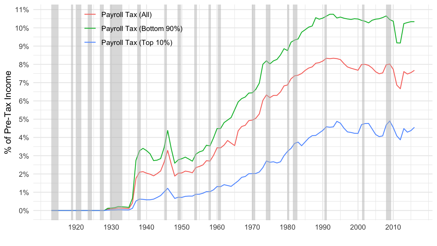
Figure 9.1: Payroll Taxes as a Percentage of Pre-Tax Income. Source: Piketty, Saez, Zucman (2018)
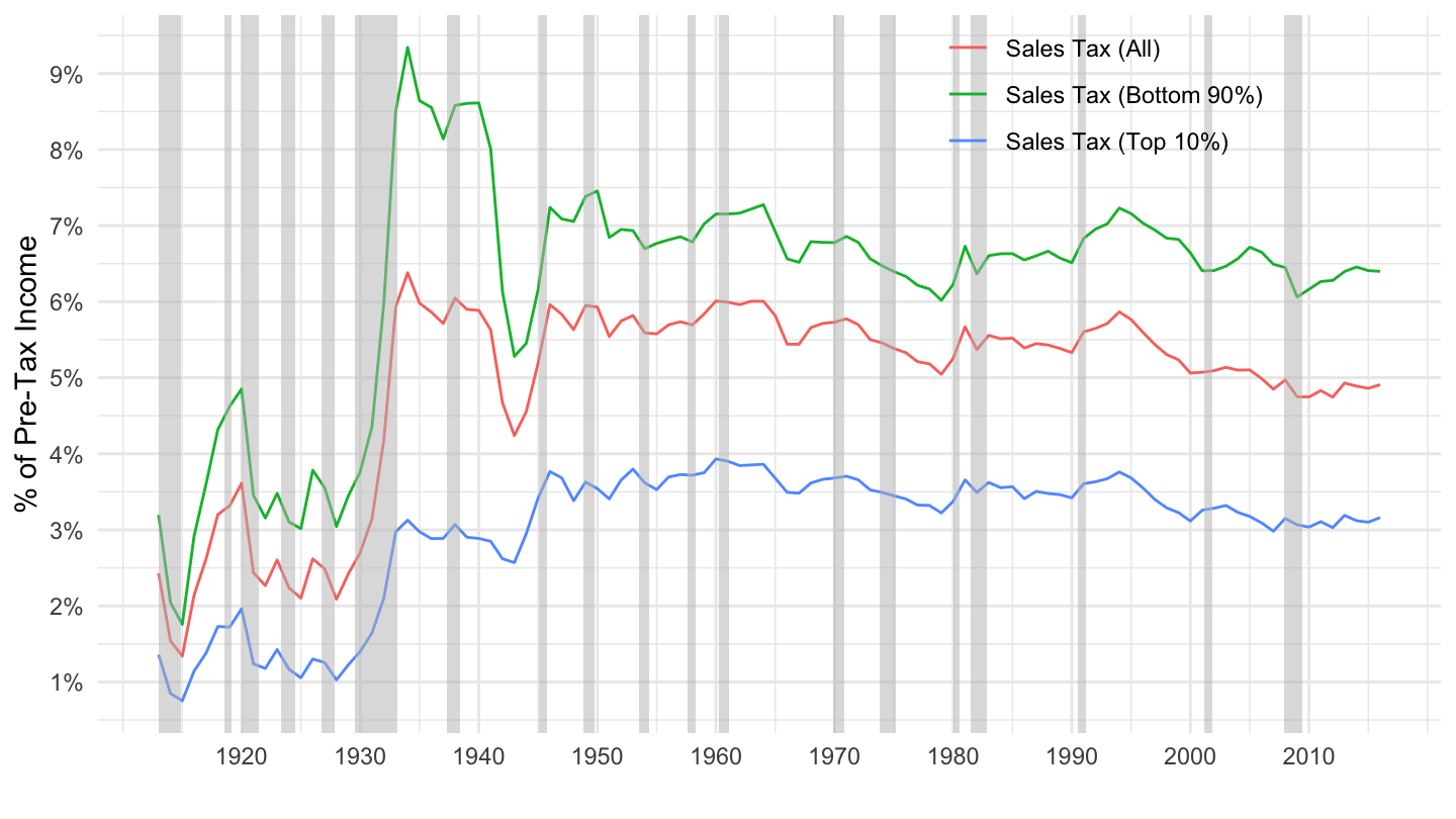
Figure 9.2: Sales Taxes as a Percentage of Pre-Tax Income. Source: Piketty, Saez, Zucman (2018)
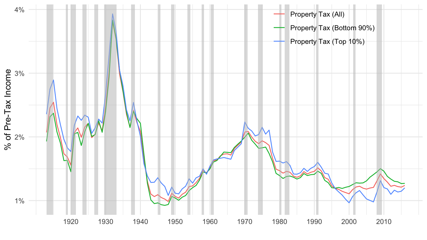
Figure 9.3: Property Taxes as a Percentage of Pre-Tax Income. Source: Piketty, Saez, Zucman (2018)
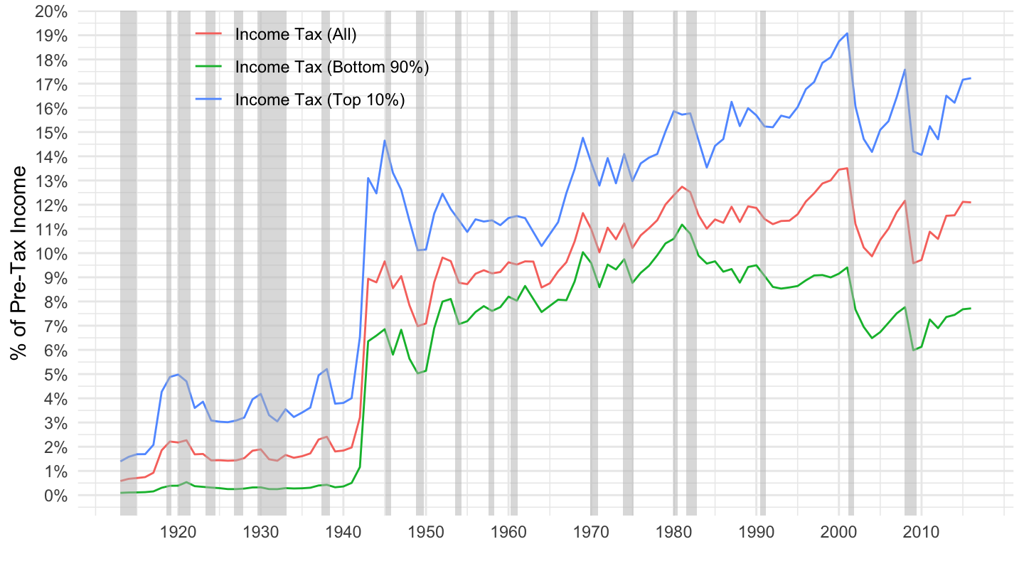
Figure 9.4: Income Taxes as a Percentage of Pre-Tax Income. Source: Piketty, Saez, Zucman (2018)
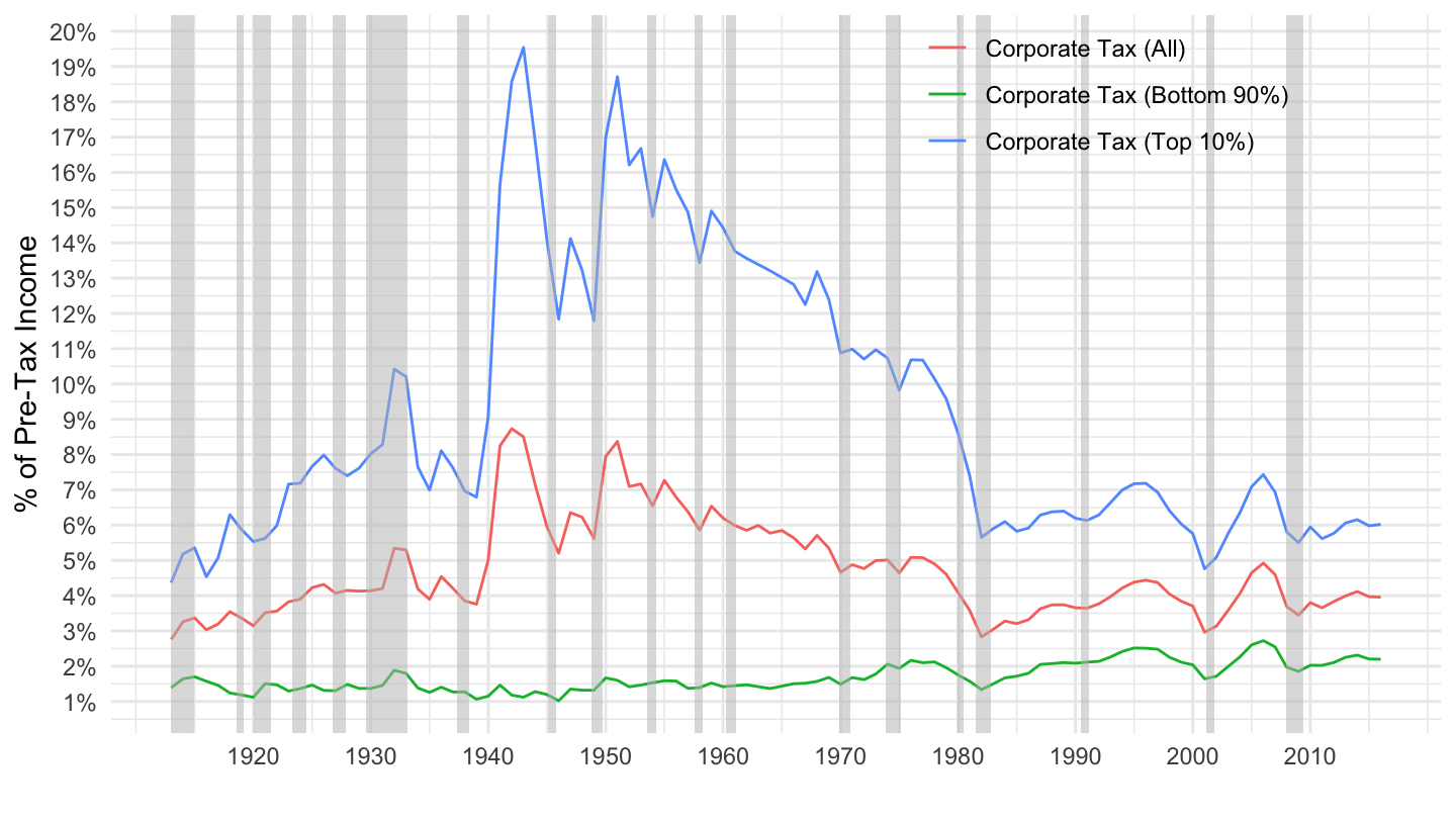
Figure 9.5: Corporate Taxes as a Percentage of Pre-Tax Income. Source: Piketty, Saez, Zucman (2018)
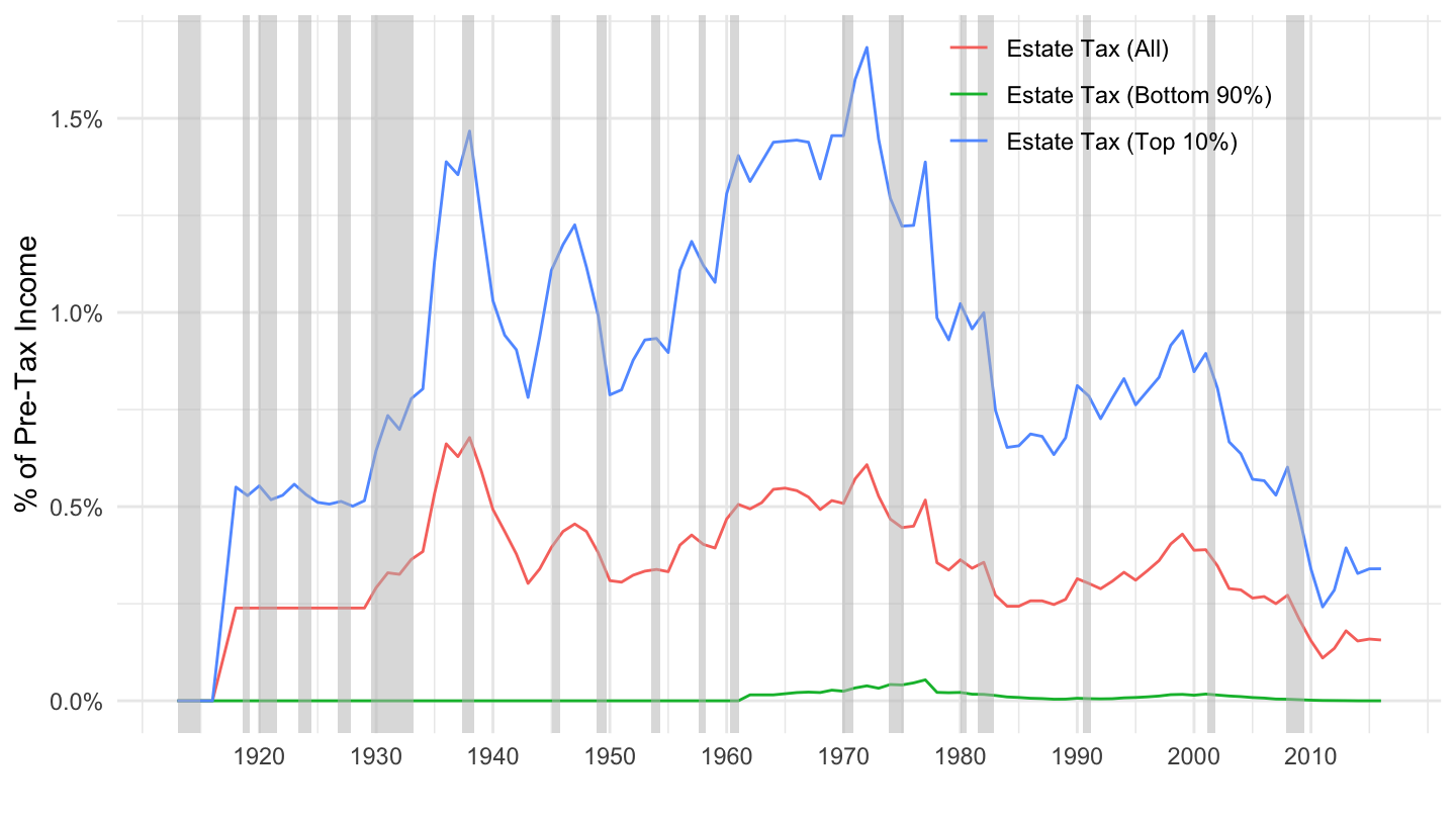
Figure 9.6: Estate Taxes as a Percentage of Pre-Tax Income. Source: Piketty, Saez, Zucman (2018)
Required readings
“Inequality Will Eventually Hurt the Rich, Too”, Michael Pettis, New York Times, April 18, 2019.
I should warn you here that we should actually not be taking a first-order condition. A mathematician would be thinking that this is wrong: the objective function is linear, and so the above function does not have a maximum ! At the same time, doing so does lead to the “right solution”. The real wage equals labor productivity in the end. What is going on here? One intuitive way to see this is to say that for any \(\alpha\), however small, then with \(f(l)=A l^{1-\alpha}\) we would get \(w/p=A \cdot l^{-\alpha}\) as a first order condition. Taking then the limit of \(\alpha\) to \(0\) then leads to the above result since then \(l^{-\alpha} \approx 1\). However, unfortunately, this is not strictly a valid mathematical proof. There is no theorem in mathematics which says that the limit of the maxima of many functions converges to the maximum of the limit of these functions. I said “unfortunately”, but this is fortunate actually, as we just found a counterexample in this exercise: the limit of the functions does not, in fact, have a maximum! It does not explain the economics, either. So how do we think of what happens if the technology is completely linear? How do we think of an equilibrium in that case? If we had \(p \cdot A>w\), then the marginal gain of hiring an additional worker would be higher than the marginal cost of doing so, whatever \(l\). Therefore, firms would like to hire an infinity of workers, and the solution would be \(l=+\infty\). This is not a competitive equilibrium, because this level of demand can never be equal to supply. If we had \(p \cdot A<w\), then the marginal gain of hiring an additional worker would be lower than the marginal cost of doing so, whatever \(l\). Therefore, the optimal thing for the firm to maximize its profit would be to hire no worker \(l=0\). This is not a competitive equilibrum either, because this level of demand is not equal to supply either.↩
You should note that with \(w/p=A\), the firms’ profit is \(0\) regardless of what \(l\) it chooses. Thus, the firm produces, potentially at a scale consistent with market clearing, but in terms of profit it is indifferent between producing or not.↩
Paul A. Samuelson. Economics: An Introductory Analysis. First Edition. Chapter 12: Saving and Investment. The full chapter is available at <bib/Samuelson1948/ch12.pdf>.↩