L Problem Set 4 - Solution
L.1 The Neoclassical Labor Market Model
This is straight from lecture 6. Labor demand is: \[l=A^{1/\alpha}(1-\alpha)^{1/\alpha}\left(\frac{w}{p}\right)^{-1/\alpha}.\] Note: If asked about this during an exam, you are required to provide the different steps. And you are not supposed to memorize this formula.
See the spreadsheet.
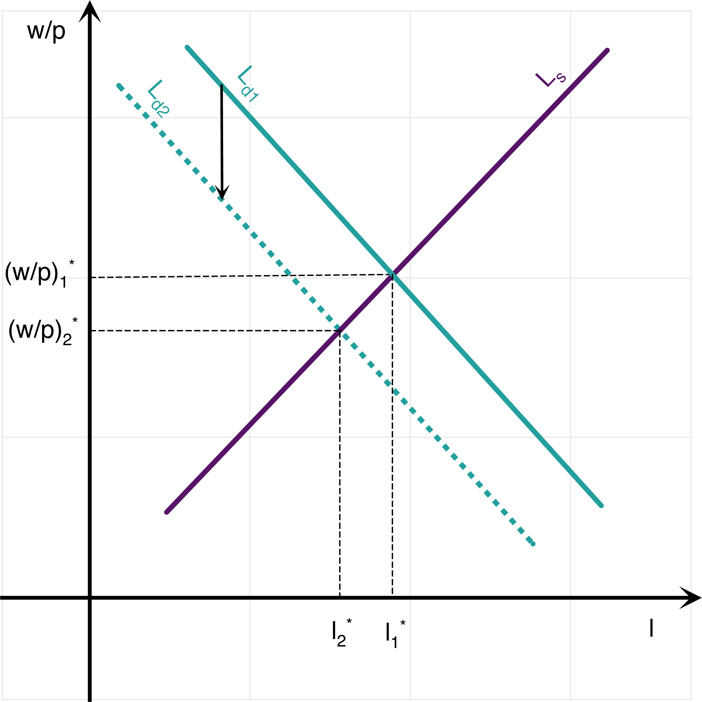
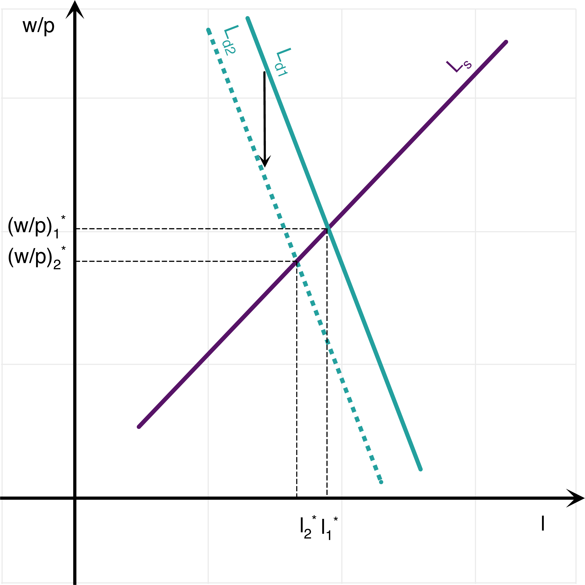
Taking logs on both sides leads to: \[\log(l)=\frac{1}{\alpha}\log A+\frac{1}{\alpha}\log(1-\alpha)-\frac{1}{\alpha}\log\left(\frac{w}{p}\right).\] Expressing the log of the real wage as a function of the log of labor demand, since the real wage is on the \(y\)-axis: \[\boxed{\log\left(\frac{w}{p}\right) = \left[\log A + \log(1-\alpha)\right] -\alpha \log(l)}.\] Therefore, it is clear that the slope of the labor demand curve is given by \(\alpha\). If \(\alpha\) is higher, then the labor demand curve is steeper. This result is intuitive: as \(\alpha\) is higher, returns to scale become more and more decreasing with respect to labor (if \(\alpha=0\), technology is constant returns in labor in constrast). Therefore, a higher quantity of labor is hired by the firm only if the real wage becomes substantially lower. (in order to “make up for” the decreasing returns) An increase in \(A\) clearly shifts the labor demand curve to the right: for a given amount of labor hired, a higher productivity implies a higher real wage, both intuitively as well as in the algebra. When the labor demand curve moves to the right, then we move along the labor supply curve, towards higher values of employment and higher real wages. A decrease in \(A\), in contrast, shifts the labor demand curve to the left, then we move down lower values of employment and lower real wages, along the labor supply curve.
Again, this is straight from lecture 6. Labor supply is: \[l=\frac{1}{B^{1/\epsilon}}\left(\frac{w}{p}\right)^{1/\epsilon}.\] Note: If asked about this during an exam, you are required to provide the different steps. And you are not supposed to memorize this formula.
See the spreadsheet. However, in order to plot the two curves on the same graphs, it is best to invert these relationship and to express the real wage as a function of labor demand \[\frac{w}{p}=A (1-\alpha)l^{-\alpha},\] and the real wage as a function of labor supply: \[\frac{w}{p}=B l^{\epsilon}.\] Again, see the second sheet of the spreadsheet for a plot where both labor supply and labor demand appear.
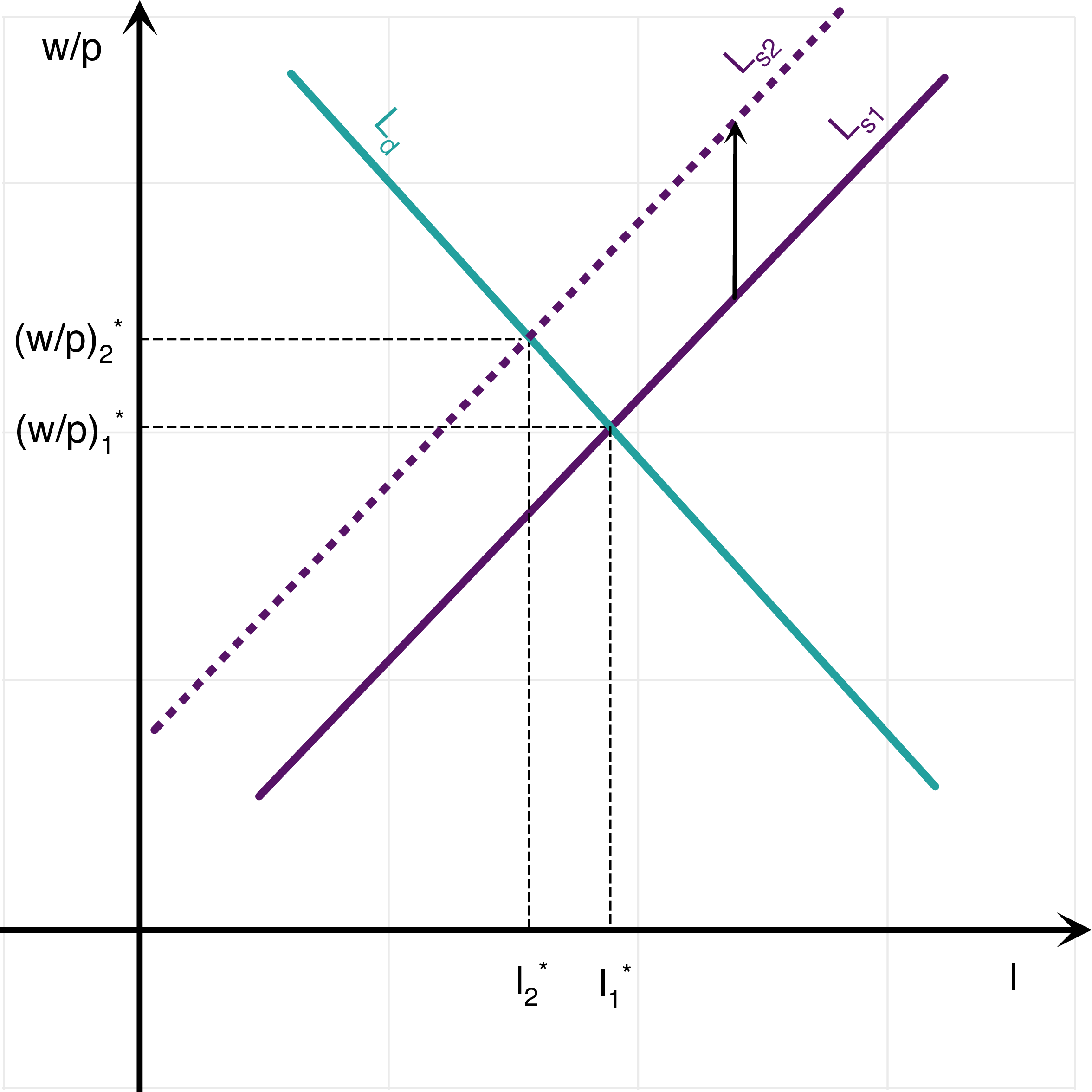
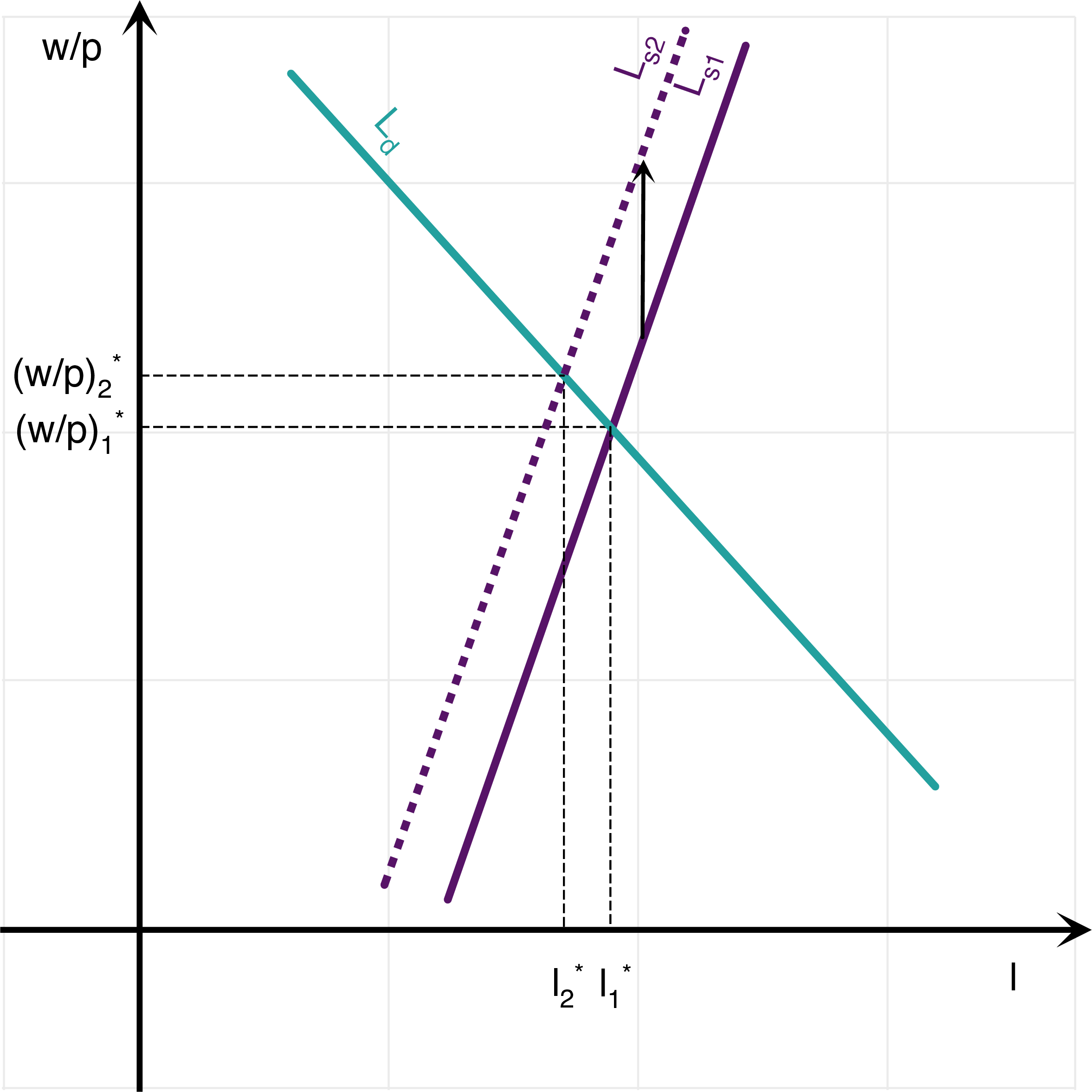
The labor supply curve is also a line in a \((\log(l), \log(w/p))\) plane, because we have a linear relationship between the log labor supply and the log real wage: \[\boxed{\log\left(\frac{w}{p}\right)=\log B + \epsilon \log(l)}.\] The slope of this supply curve on a log-log graph is given by \(\epsilon\). If \(\epsilon\) is larger, the slope is larger. This is intuitive: if the disutility of labor is more convex, then people dislike more working extra hours, and need to be compensated by a much higher real wage to do it. Clearly, if \(B\) increases, the labor supply curve moves to the left: people get more disutility from working, and they need to be compensated by a higher real wage to work the same number of hours. On the contrary, when \(B\) decreases, people enjoy working much more, and so employers may pay them a low wage to do so.
There are many ways to answer this question. I will provide just two. One is to derive the expressions in lecture 6, using the original versions of labor supply and demand (without logs). The real wage is: \[\frac{w}{p} = (1-\alpha)^{\frac{\epsilon}{\alpha+\epsilon}}A^{\frac{\epsilon}{\alpha+\epsilon}} B^{\frac{\alpha}{\alpha+\epsilon}}.\] The level of employment: \[l= (1-\alpha)^{\frac{1}{\alpha+\epsilon}}A^{\frac{1}{\alpha+\epsilon}} B^{-\frac{1}{\alpha+\epsilon}}\] Using the spreadsheet, and plugging in the values for \(A_1 = 2\), \(A_2 = 1.9\), we get: \[ \begin{aligned} l_1 &=0.9267933073, \qquad \left(\frac{w}{p}\right)_1=1.367553862\\ l_2 &=0.9179226047, \qquad \left(\frac{w}{p}\right)_2=1.303347791 \end{aligned} \] The effects of employment of a change in \(A\) given by \((A_2-A_1)/A_1=-5\%\), are thus a fall in employment and in real wages given by: \[\frac{l_2-l_1}{l_1}=-0.96\%, \qquad \frac{\left(\frac{w}{p}\right)_2-\left(\frac{w}{p}\right)_1}{\left(\frac{w}{p}\right)_1}=-4.69\%.\] In log changes: \[\log(l_2)-\log(l_1)=-0.96\%, \qquad \log\left(\frac{w}{p}\right)_2-\log\left(\frac{w}{p}\right)_1=-4.81\%.\] Or we combine the logged versions of these same equations: \[\log\left(\frac{w}{p}\right) = \left[\log A + \log(1-\alpha)\right] -\alpha \log(l).\] and labor supply: \[\log\left(\frac{w}{p}\right)=\log B + \epsilon \log(l)\] we get that: \[ \begin{aligned} \log B &+ \epsilon \log(l) = \left[\log A + \log(1-\alpha)\right] -\alpha \log(l)\\ & \quad \Rightarrow \quad \log(l)=\frac{1}{\epsilon + \alpha}\left[\log A + \log(1-\alpha) - \log B\right] \end{aligned} \] We may use either the labor demand curve or the labor supply curve to compute the real wage (if everything goes well, they should both give the same answer). We can plug it back in the supply curve: \[ \begin{aligned} \log\left(\frac{w}{p}\right)&=\log B+\frac{\epsilon}{\epsilon + \alpha}\left[\log A + \log(1-\alpha) - \log B\right]\\ \log\left(\frac{w}{p}\right)&=\frac{\alpha}{\epsilon+\alpha}\log B + \frac{\epsilon}{\epsilon + \alpha} \log A +\frac{\epsilon}{\epsilon + \alpha}\log(1-\alpha) \end{aligned} \] Therefore, we get the equilibrium employment: \[\boxed{\log(l)=\frac{1}{\epsilon + \alpha}\left[\log A + \log(1-\alpha) - \log B\right]},\] as well as the equilibrium real wage: \[\boxed{\log\left(\frac{w}{p}\right)=\frac{\alpha}{\epsilon+\alpha}\log B + \frac{\epsilon}{\epsilon + \alpha} \log A +\frac{\epsilon}{\epsilon + \alpha}\log(1-\alpha)}.\] This implies that, following a change in productivity \(A\):: \[\Delta \log(l) = \frac{1}{\epsilon+\alpha} \Delta \log A\] \[\Delta \log\left(\frac{w}{p}\right) = \frac{\epsilon}{\epsilon+\alpha} \Delta \log A\] The change in \(A\) in log points is: \[\Delta \log A=\log(A_2)-\log(A_1)=-5.13\%.\] Therefore, in log changes: \[\log(l_2)-\log(l_1)=-0.96\%, \qquad \log\left(\frac{w}{p}\right)_2-\log\left(\frac{w}{p}\right)_1=-4.81\%.\] If \(\alpha\) is higher, then from the above formula the change in employment and in the real wage is lower: \[\Delta \log(l) = \frac{1}{\epsilon+\alpha} \Delta \log A\] \[\Delta \log\left(\frac{w}{p}\right) = \frac{\epsilon}{\epsilon+\alpha} \Delta \log A\] The economic intuition is that a change in \(A\) shifts the labor demand curve, and leads to a movement along the labor supply curve. However, the size of this shock is dampened, the larger the amount of decreasing returns to scale. Graphically, the shift in the labor demand curve from a given change shift along the y-axis is lower when the slope is larger. This is shown on the two figures below, showing the shift in the labor demand curve from a given change in \(A\) (along the y-axis), when \(\alpha\) is low (low decreasing returns) on the left hand side and when \(\alpha\) is high (high decreasing returns) on the right hand side. Note: You may play around with the spreadsheet to see what happens when parameters are changed.
- (Warning! if this idea of an increase in leisure attractiveness seems a bit peculiar to you, it also seems odd to me. But it has been proposed by some economists as an explanation for unemployment, to explain why the real wage did not fall that much during the recession.) Similar calculations on the spreadsheet and using the same formulas: \[\frac{w}{p} = (1-\alpha)^{\frac{\epsilon}{\alpha+\epsilon}}A^{\frac{\epsilon}{\alpha+\epsilon}} B^{\frac{\alpha}{\alpha+\epsilon}}.\] The level of employment is: \[l= (1-\alpha)^{\frac{1}{\alpha+\epsilon}}A^{\frac{1}{\alpha+\epsilon}} B^{-\frac{1}{\alpha+\epsilon}}\] imply that a 10 per cent increase in \(B\) leads to a reduction in employment and an increase in real wages given by: \[\log(l_2)-\log(l_1)=-1.79\%, \qquad \log\left(\frac{w}{p}\right)_2-\log\left(\frac{w}{p}\right)_1=0.60\%.\] If \(\epsilon\) is higher, then the effect on both employment and real wages is smaller in absolute value. Again, this is intuitive: if labor supply is steeper to begin with, then a given increase in \(B\) does not lead to as much of a shift in the labor supply curve. Thus, the move along the labor demand curve towards lower employment and higher wages is not as important then. This is shown on the two figures below, where the increase in leisure attractiveness is the same across the two experiments: on the left-hand side, epsilon is low, while on the right hand side, epsilon is high. Note: Again, you may play around with the spreadsheet to see what happens when parameters are changed.
L.2 The “Keynesian” Labor Market Model
One way to answer this question is to note that with a fall in productivity, the labor demand curve will shift to the left (as in lecture 6). If real wages are rigid, then workers are off their labor supply curve (they would like to work more at the current wage) but still on firms’ labor demand curve: \[\log\left(\frac{w}{p}\right) = \left[\log A + \log(1-\alpha)\right] -\alpha \log(l).\] For a given change in \(\Delta \log A\), the change in employment is therefore simply given by the previous expression through: \[\Delta \log(l)=\frac{\Delta \log A}{\alpha}.\] In contrast, in the previous case, with flexible wages, the change in employment following a productivity shock was only: \[\Delta \log(l) = \frac{\Delta \log A}{\epsilon+\alpha}.\] Given a change in productivity of \(5\%\), which goes from \(2\) to \(1.9\), or \(\log(1.9)-\log(2)=5.13\%\) in log points, we get a drop of \(15.39\%\) in log points in employment: \[\log(l_2)-\log(l_1)=-15.39\%.\]
In question 7 of the previous exercise, we got in contrast a change: \[\log(l_2)-\log(l_1)=-0.96\%,\] a much smaller number. The intuition was that the wage falling incentivizes employers to hire more workers. Here, in contrast, because the wage is “too high” and cannot fall by definition, employers do not want to hire them.
We know from lecture 6 that if leisure becomes more attractive, then employment must fall and the real wage must rise. We imagine here that wages are sticky upwards. Then, people will be off firms’ labor demand curves, but on their labor supply curves. Thus, it is still true that: \[\log\left(\frac{w}{p}\right)=\log B + \epsilon \log(l).\] For a given change in \(\Delta \log B\), given that wages are sticky, the change in employment is therefore simply given by the previous expression through: \[\Delta \log(l)=-\frac{\Delta \log B}{\epsilon}.\] In contrast, in the previous case, with flexible wages, the change in employment following a \(B\) shock was only: \[\Delta \log(l) =- \frac{\Delta \log B}{\epsilon+\alpha}.\] Given an increase in \(B\) of \(10\%\), which goes from \(2\) to \(2.2\), or \(\log(2.2)-\log(2)=9.53\%\) in log points, we get a drop of \(1.91\%\) in log points in employment: \[\log(l_2)-\log(l_1)=-1.91\%.\]
In question 8 of the previous exercise, we got in contrast a change: \[\log(l_2)-\log(l_1)=-1.79\%,\] a somewhat smaller number. The intuition was that the wage increasing would have incentivized workers to work more. But because wages are sticky, this did not happen.
L.3 The Bathtub model
Assume a monthly job separation rate equal to \(s=1\)%, and a monthly job finding rate equal to \(f=20\)%. Assume that the labor force is given by \(L=159\) million.
The steady state unemployment rate is obtained by equating separations and job findings in the steady state, so that: \[ \begin{aligned} &s E^{*} = f U^{*} \quad \Rightarrow \quad sL - s U^{*} = fU^{*}\\ &\quad \Rightarrow \quad U^{*}=\frac{s}{s+f}L \quad \Rightarrow \quad u^{*}=\frac{s}{s+f}. \end{aligned} \] The steady state unemployment rate \(u^{*}\), number of people unemployed \(U^{*}\), and number of people losing or finding a job each month, are given by (see the spreadsheet): \[u^{*}=4.76\%, \quad U^{*}=7,571,429, \quad f U^{*} = 1,514,286.\]
Again, there are many ways we can proceed here. One is to use the spreadsheet to iterate on the law of motion, that is calculate \(u_{t+1}\) as a function of \(u_t\) and then see graphically when the given unemployment rate is reached. The law of motion is: \[U_{t+1}-U_t = s(L-U_t) -f U_t.\] Thus (see lecture 6): \[U_{t+1}=sL + \left(1-s-f\right)U_t.\] Dividing both sides by \(L\), and denoting by \(u_{t}=U_t/L\) the rate of unemployment: \[u_{t+1}=s+\left(1-s-f\right)u_t.\] We find that the unemployment rate reaches 5% after approximately 11 months (the unit of time is one month). A second method is to do a bit of algebra before using the computer. We write the law of motion for unemployment (again, see lecture 6 for details): \[ \begin{aligned} &U_{t+1}-U_t = s(L-U_t) -f U_t \\ & \quad \Rightarrow \quad U_{t}-U^{*}=(1-s-f)^t\left(U_0-U^{*}\right). \end{aligned} \] Dividing everything by \(L\) gives everything in terms of unemployment rates: \[u_{t}=(1-s-f)^t\left(u_0-u^{*}\right) + u^{*}.\] Thus, starting from an unemployment rate \(u_0\) it is possible to get a value for all subsequent \(u_t\), using the above formula. We may then use the spreadsheet to compute this and find that the unemployment rate reaches 5% after approximately. Again find that the unemployment rate reaches 5% after approximately 11 months (the unit of time is one month). A third method is to in fact do all the algebra and calculate the time \(T\) we are looking for explicitely. We are looking for \(T\) such that \(u_t \leq \bar{u}=5\%\) for \(t \geq T\). This implies: \[ \begin{aligned} &(1-s-f)^t\left(u_0-u^{*}\right) + u^{*} \leq \bar{u}\\ &\quad \Rightarrow \quad (1-s-f)^t \leq \frac{\bar{u}-u^{*}}{u_0 - u^{*}} \\ & \quad \Rightarrow \quad t \log(1-s-f) \leq \log\frac{\bar{u}-u^{*}}{u_0 - u^{*}} \\ & \quad \Rightarrow \quad t \geq \frac{\log\frac{\bar{u}-u^{*}}{u_0 - u^{*}}}{\log(1-s-f)}. \end{aligned} \] (be careful, \(\log(1-s-f)\) is negative because \(1-s-f\) is lower than \(1\) so you have to change the inequality from \(\leq\) to \(\geq\)). A numerical application using the spreadsheet shows that this condition means: \[t \geq 11.07.\] The advantage of this method is we know exactly when the unemployment rate reaches 5%. After 11.07 months ! (given the simplicity of the model, displaying the second digit does not make much sense, though)
We are looking for \(f\) such that: \[u^{*}=\frac{s}{s+f}\quad \Rightarrow \quad f=\frac{s}{u^{*}}-s,\] which implies using these numbers that: \[f=40\%.\] This is intuitive: you have double the separation rate, you want double the job finding rate for the unemployment rate to be the same in the steady-state. Indeed, in the steady state: \[s E^{*}=f U^{*}.\] Therefore, if the unemployment rate is the same, then if \(s\) doubles \(f\) must double as well.
See question 2. The spreadsheet should give all the answers. We find: \[t \geq 4.79.\] Thus, the unemployment rate reaches 5 per cent after approximately 5 months.
The answer is very much contained in questions 2 and 4. If the rates of job separations and job finding are higher like they typically are in America, the unemployment rate reaches its steady-state value faster. This may explain why the United States are able to recover faster from shocks than, say, Spain or Italy (at least in terms of unemployment rates). Here is some supporting evidence that the unemployment rate is more persistent in Europe than in America:
https://db.nomics.world/OECD/EO/USA.UNR.Q
https://db.nomics.world/OECD/EO/ESP.UNR.Q
https://db.nomics.world/OECD/EO/ITA.UNR.Q