7 The Multiplier
Link to slides / Link to handouts
This lecture opens a set of lectures on Keynesian economics. The neoclassical models of consumption, saving, investment, and the labor market that we have studied so far are quite close to what the mainstream paradigm was teaching when John Maynard Keynes started to think about these issues. J.M. Keynes refers to this paradigm as “classical”. Yet, according to him, this paradigm was not a general one, in that it did not apply to a case where there was an insufficient use of resources. According to him, the U.S. after the Great Depression was in such a situation, where the teaching of traditional economics was therefore “misleading and disastrous”. The first chapter of the General Theory starts with these words:
I have called this book the General Theory of Employment, Interest and Money, placing the emphasis on the prefix general. The object of such a title is to contrast the character of my arguments and conclusions with those of the classical theory of the subject, upon which I was brought up and which dominates the economic thought, both practical and theoretical, of the governing and academic classes of this generation, as it has for a hundred years past. I shall argue that the postulates of the classical theory are applicable to a special case only and not to the general case, the situation which it assumes being a limiting point of the possible positions of equilibrium. Moreover, the characteristics of the special case assumed by the classical theory happen not to be those of the economic society in which we actually live, with the result that its teaching is misleading and disastrous if we attempt to apply it to the facts of experience.
According to J.M. Keynes, the type of models we have seen so far are special in that they only apply in a case where there is full employment of resources. In contrast, underutilization of resources requires a different approach. In the model that we will study today, consumption does not result from intertemporal optimization, as in lecture 2 and lecture 4 but from a mechanical “consumption function” relating consumption to current income. Investment is not be determined by the supply of saving as in the Solow growth model of lecture 1.5, but by the demand for investment by firms. Finally, there may exist involuntary unemployment, unlike in the neoclassical model of lecture 6. Workers are potentially off their labor supply curve: they would be willing to take a job at the current wage. In J.M. Keynes’ view of the world, an increase in demand can therefore potentially be met by an increase in supply, because some labor is idle and ready to be used in production.
During this lecture, I first go through the various components of aggregate demand in section 7.1. I then go through a presentation of the simple Keynesian goods market model in section 7.2, and then present a couple of variations on the Keynesian goods market model in section ??: automatic stabilizers, and “accelerator” effects of output on investment.
The assumptions and logic of the Keynesian theory may be a little disturbing at first:
The difficulty lies, not in the new ideas, but in escaping from the old ones, which ramify, for those brought up as most of us have been, into every corner of our minds.
7.1 The Demand for Goods
Consider the first accounting identity of lecture 1, showing the different components of the demand for goods: \[Y=C+I+G+X-M.\] The total demand for goods is determined by consumption demand, investment demand, government spending, and net exports (for example, China’s total demand includes US’ demand for Chinese products).
For simplicity, we shall assume for now that we are considering a closed economy - think, for example, of the world economy - so that there are no exports or imports: \[X=M=0 \quad \Rightarrow \quad NX=0.\]
This assumption, which is not satisfying as the policies we shall consider are national (fiscal policy, etc.), will be relaxed starting in lecture 11. In lecture 1.5 and lecture 4, output was also determined by the amount of available technology, as well as by the supply of labor \(L\), and of capital \(K\) in the economy (the “supply side”): \[Y=F\left(K, L\right).\] For example, in the Solow growth model of lecture 1.5, where government spending was zero (\(G=0\)), GDP was simultaneously equal to \(F(K,L)\) as well as to \(C+I\). This is what allowed us to derive the dynamics in the economy.
In the Keynesian model, output is determined only by aggregate demand. The underlying assumption is that there exists some idle resources which allow to accommodate any increase in demand by an increase in labor utilization. In order to show that output is determined by demand, we shall denote the total demand for goods by \(Z\): \[Z=C+I+G.\] The Keynesian assumption then is that output is demand determined, so that: \[Y=Z.\] We shall now investigate these components of demand in turn.
Consumption Demand. The first (and largest) component of the demand for goods comes from consumption. Rather than starting from microeconomic principles of optimization under constraints, J.M. Keynes postulates a consumption function relating disposable income to consumption. In its most general form, consumption is simply a function of disposable income \(Y_D\), disposable income being the income that remains once consumers have received transfers from the government and paid their taxes: \[C=C(Y_D), \quad \frac{dC}{dY_D}>0.\] The positive derivative implies that when disposable income goes up, people buy more goods; when it goes down, they buy fewer goods. It is often useful to specify a functional form for this consumption function, such as: \[C(Y_D)=c_0+c_1Y_D.\] In this case, the consumption function has a linear relation. This linear relation has two parameters:
- \(c_1\) is called the marginal propensity to consume. It gives the effect of an additional dollar of income on consumption. For instance, if \(c_1=0.7\) (\(c_1=70\%\)), then an additional dollar of disposable income increases consumption by 1 dollar times 0.7, or 70 cents. A natural restriction on \(c_1\) is that it is positive: an increase in disposable income should (at least averaging across individuals) lead to an increase in consumption. Another natural restriction on \(c_1\) is that it be less than \(1\): people are likely to save some of their increase in disposable income. Keynes presents this as follows in Chapter 10 of the General Theory:
Our normal psychological law that, when the real income of the community increases or decreases, its consumption will increase or decrease but not so fast, can, therefore, be translated - not, indeed, with absolute accuracy but subject to qualifications which are obvious and can easily be stated in a formally complete fashion into the propositions that \(\Delta C_w\) and \(\Delta Y_w\) have the same sign, but \(\Delta Y_w > \Delta C_w\), where \(C_w\) is the consumption in terms of wage-units. This is merely a repetition of the proposition already established in Chapter 3 above. Let us define, then, \(dC_w/dY_w\) as the marginal propensity to consume.
- \(c_0\) corresponds to what people would consume if their disposable income was equal to \(0\) (for instance, they would still need to eat). In most instances, they would still be able to eat by running down their saving, or borrowing from banks. In terms of the model, changes in \(c_0\) should be thought of as everything that moves consumption without going through disposable income directly. This might therefore proxy for consumer confidence, the willingness of banks to lend to consumers, etc.
Finally, disposable income is defined as: \[Y_D \equiv Y - T,\] where \(Y\) is income and \(T\) is taxes paid minus government transfers received by consumers. Very often, we will refer to \(T\) as “taxes”, which will always imply “net taxes”, unless otherwise specified.
Finally, note that “income” includes here both labor income as well as capital income, and is therefore equal to GDP. The underlying assumption is that \(c_1\) represents a weighted average of marginal propensity to consume across people with different incomes, and different types of incomes.
Investment Demand. The second component of the demand for goods is coming from investment demand. In the Solow growth model, investment was determined by saving. For the Keynesian model, we shall make two alternative assumptions about investment:
In the baseline version of the model, we shall assume that investment is fixed: \[I=\bar{I}.\] In order to remind ourselves that investment is fixed (or “exogenous”, that is, determined outside of the model), we shall denote investment by “I bar” \(\bar{I}\).
In the investment accelerator version of the model, we shall assume in contrast that investment depends on output. This assumption is more realistic in practice: an Italian restaurant which has many customers is more likely to renovate it and to buy a new pizza oven. In this case, we will assume that investment depends on output in a linear way: \[I=b_0+b_1 Y.\]
Government Spending. The third and final component of demand in our closed economy model is government spending \(G\). Together with net taxes \(T\) representing the tax-and-transfer system, \(G\) is a component of fiscal policy. We shall also take \(G\) as exogenous, but we will study the impact of alternative values for \(G\) for the determination of GDP, for example (when we talk about the multiplier).
7.2 The Simple Goods Market Model
The Simple Goods Market Model, also called the (ZZ)-(YY) model, assumes a closed economy, that investment is exogenous and equal to \(\bar{I}\), an exogenous government spending \(G\), and a consumption function given as above by: \[C=c_0+c_1\left(Y-T\right).\]
(ZZ) curve. With these assumptions, and assuming a closed economy, the value of the demand for goods \(Z\) is: \[ \begin{aligned} Z &=C+\bar{I}+G\\ &=c_{0}+c_{1}\left(Y-T\right)+\bar{I}+G\\ Z &=\left(c_{0}+\bar{I}+G-c_{1}T\right)+c_{1}Y \end{aligned} \] This determines a value for the demand for goods \(Z\), as a function of aggregate income, or GDP \(Y\), which defines the (ZZ) curve. The part of this demand which does not depend on income is called autonomous spending \(z_0\) defined as: \[z_0=c_{0}+\bar{I}+G-c_{1}T.\] This autonomous spending \(z_0\) is also the value of demand when income is equal to \(Y=0\). Therefore, the demand for goods \(Z\) is given as: \[Z=\underbrace{\left(c_{0}+\bar{I}+G-c_{1}T\right)}_{\text{Autonomous Spending }z_{0}}+\underbrace{c_{1}}_{\text{MPC}}Y\]
(YY) curve. Equilibrium in the goods market requires that: \[Z=Y.\] Indeed, income is determined by the total demand for goods.
Equilibrium. Equilibrium is determined by the intersection of the (YY) and the (ZZ) curves, represented by point A on the Figure below. Replacing out \(Z=Y\) in the expression for \(Z\) above indeed implies: \[Y=\left(c_{0}+\bar{I}+G-c_{1}T\right)+c_{1}Y.\] Therefore, putting all \(Y\) terms of the left-hand side: \[Y=\underbrace{\frac{1}{1-c_{1}}}_{\text{Multiplier}}\times\underbrace{\left(c_{0}+\bar{I}+G-c_{1}T\right)}_{\text{Autonomous Spending }z_{0}}.\]
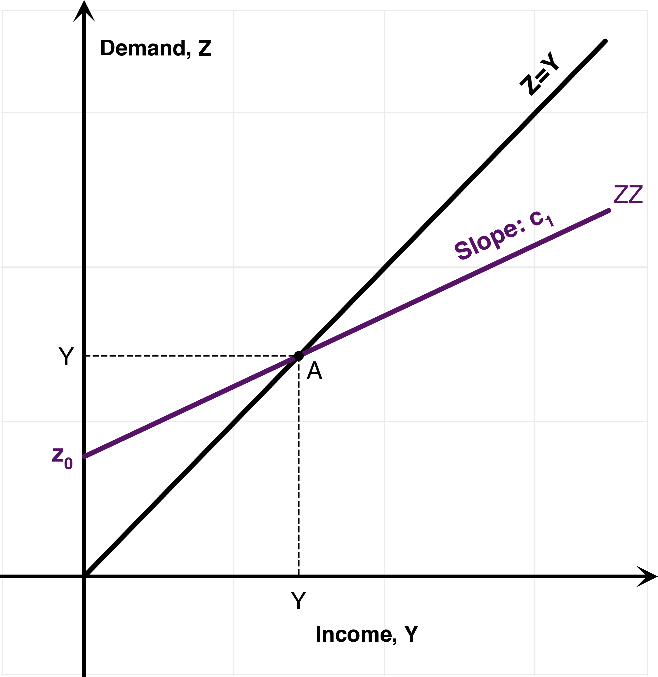
Figure 7.1: The Simple Goods Market (ZZ)-(YY) model.
Multiplier. Consider a change in autonomous spending \(\Delta z_{0}=z_{0}'-z_{0}\) coming from a change in government spending \(\Delta z_{0}=\Delta G\), or from a change in net taxes \(\Delta z_{0}=-c_{1}\Delta T\). We have: \[\Delta Y=\frac{\Delta z_{0}}{1-c_{1}}.\] By definition, the multiplier gives the increase in income which is brought about by the increase in autonomous spending. Therefore, the multiplier is given by: \[\text{Multiplier}=\frac{1}{1-c_{1}}.\] As a consequence steepness of the (ZZ) curve determines the value for the multiplier. The closer to one the slope \(c_1\) is, the higher the value of the Keynesian multiplier.
Government expenditure multiplier; tax multiplier. An increase in government spending \(\Delta G>0\) leads to an increase in output given by: \[\Delta Y=\frac{\Delta G}{1-c_{1}}.\] Thus, \(1/(1-c_1)\) is usually called the government expenditure multiplier.
On the other hand, a decrease in net taxes \(\Delta T<0\) leads to an increase in output given by: \[\Delta Y = - \frac{c_1 \Delta T}{1-c_{1}}.\] For this reason, \(c_1/(1-c_1)\), or \(-c_1/(1-c_1)\) is sometimes called the tax multiplier.
Four interpretations. Why is the change in output higher than the change in autonomous spending? And why is it equal to \(1/(1-c_1)\), where \(c_1\) is the marginal propensity to consume. There are actually four different ways to see this, 2 are algebraic, and 2 are geometric:
Algebra. The first way to see this is just, as above to equate output to demand \(Y=Z\), which allows to get at the result.
Infinite sum of a geometric series. 1$ of additional autonomous spending brings in a second round \(c_{1}\)$ increase in consumption, a third round \(c_{1}^{2}\)$ increase in consumption, which add up to: \[\sum_{i=0}^{n}c_{1}^{i}=1+c_{1}+c_{1}^{2}+...+c_{1}^{n}=\frac{1-c_{1}^{n+1}}{1-c_{1}}.\] Therefore, because \(0<c_{1}<1\), we have: \[\text{Multiplier}=\sum_{i=0}^{+\infty}c_{1}^{i}=\frac{1}{1-c_{1}}.\]
Graphical interpretation 1. The left-hand panel of Figure 7.2 gives a graphical interpretation to this infinite geometric sum. This graphical interpretation makes it clear that: \[Y'-Y=\sum_{i=0}^{+\infty}c_{1}^{i}=\frac{1}{1-c_{1}}.\] This graph should make clear why the model is called a “Keynesian cross”. This is because the (ZZ) and (YY) curves cross to determine output. This pedagogical device to visualize the Keynesian multiplier was introduced in 1948 by Paul Samuelson in his famous Economics textbook, to provide a geometric intuitive interpretation of Keynes’ ideas.
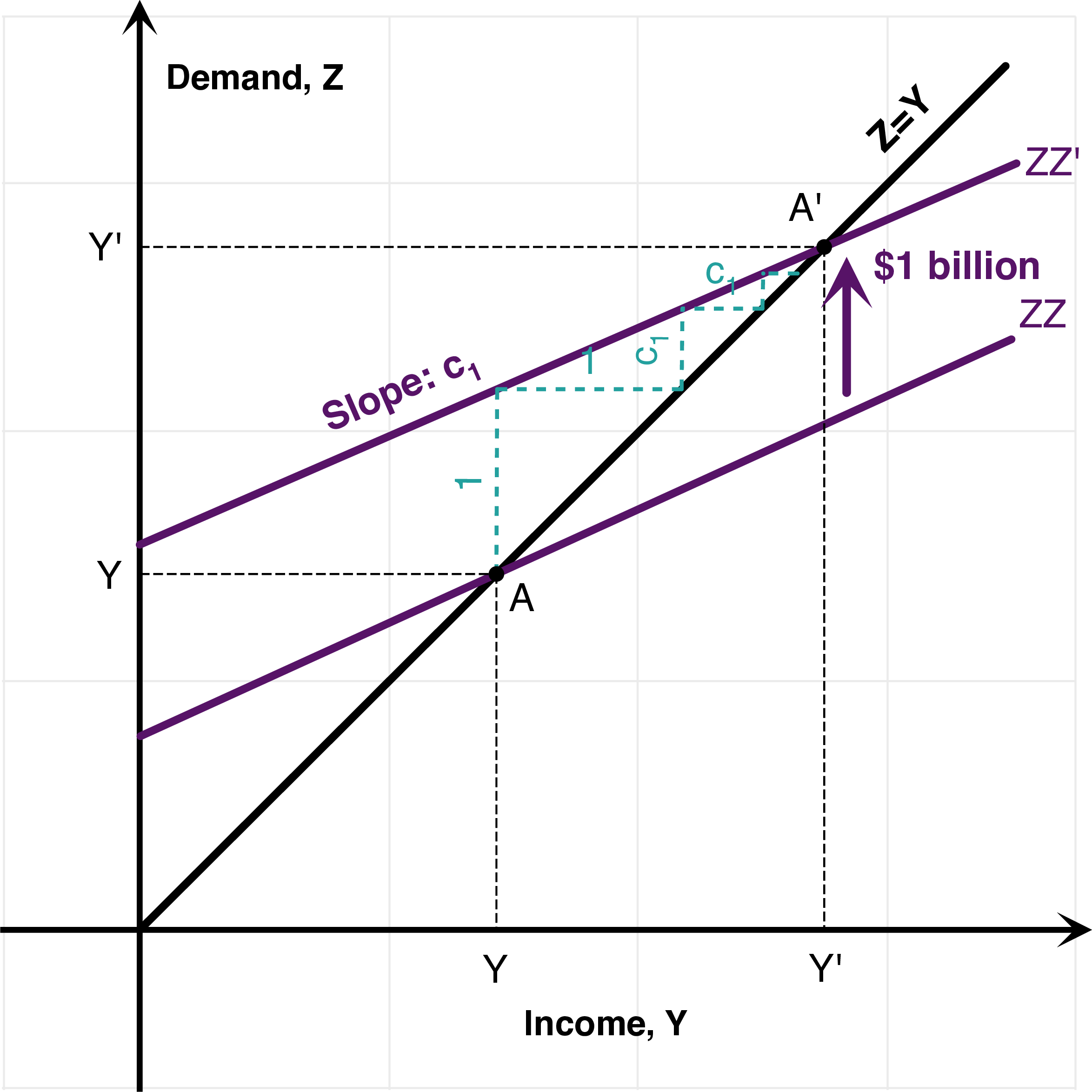
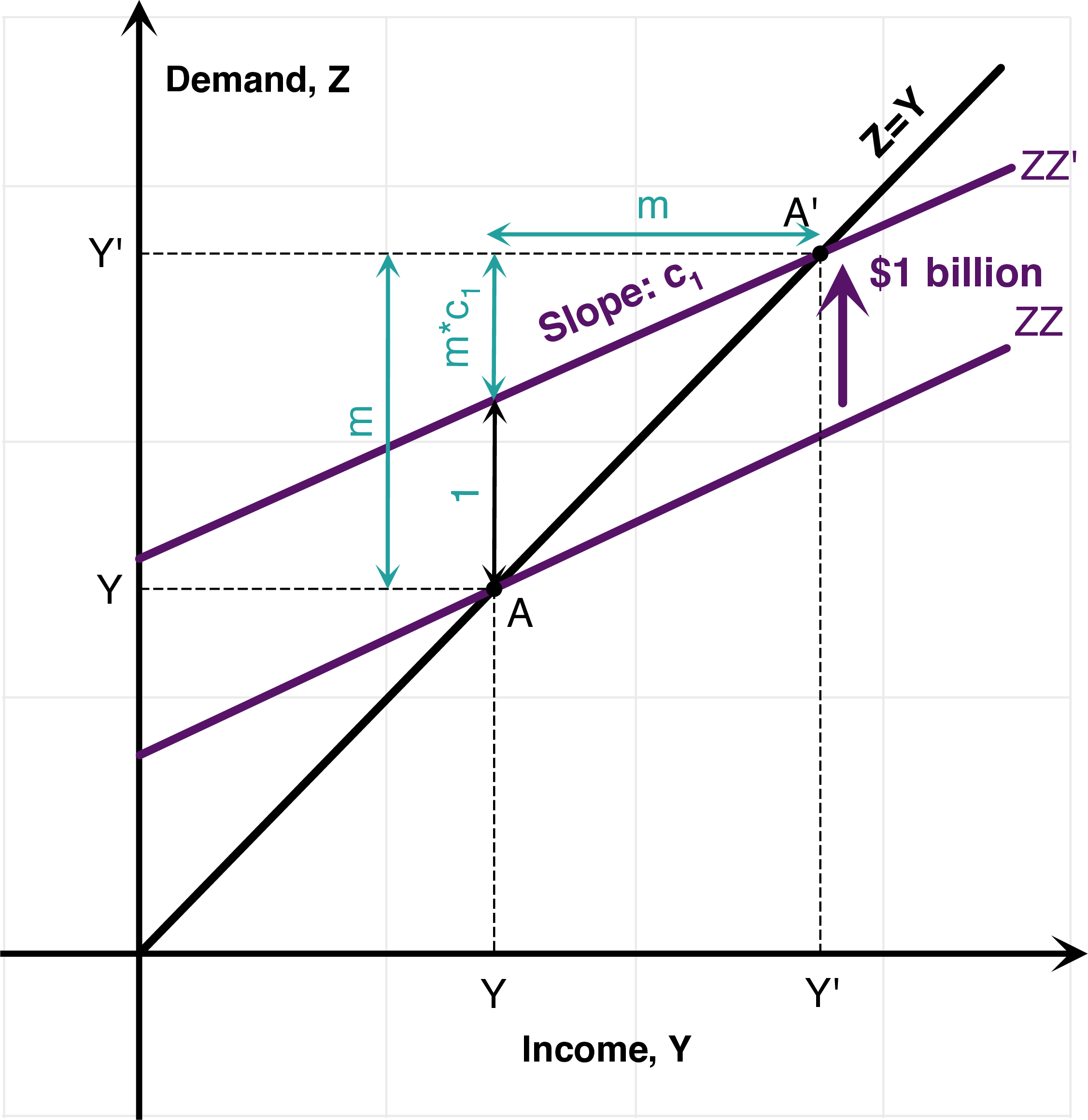
Figure 7.2: Simple Keynesian Cross: Graphical Interpretations.
- Graphical interpretation 2. The right-hand panel of Figure 7.2 gives a graphical interpretation which does not use a geometric sum. If \(m\) is the unknown value of the multiplier, then the geometry makes clear that \(m\) has to satisfy \(m=1+mc_{1}\) which also gives the value for the multiplier: \[m=1+mc_{1} \quad\Rightarrow\quad m=\frac{1}{1-c_{1}}.\]
There are multiple extensions of the Goods Market Model: one with automatic stabilizers, one with an accelerator effect of demand on investment.
7.3 Automatic Stabilizers
In practice, the tax and transfer system is designed in such a way that taxes strongly depend on the level of income: net taxes are said to be procyclical:
Many taxes, such taxes on wage income, profits, capital gains, mechanically collect more in revenues when income rises: taxes are procyclical (they vary positively with the state of the business cycle).
On the contrary, many transfers are countercyclical (they vary negatively with the state of the business cycle): when unemployment is high and income is low, more unemployment benefits or food stamps are being paid.
Overall, these two effects reinforce themselves so that net taxes are procyclical. In terms of the model, we model this by postulating a linear function for net taxes which depends on the value for income: \[T=t_{0}+t_{1}Y,\] where \(t_1 \in [0,1]\) indexes the cyclicality of net taxes with GDP.
For example, assume that \(t_1=0.3\) or 30%. Then if income rises by 1 dollar, net taxes rise by 30 cents. Using this expression for taxes allows us to write: \[ \begin{aligned} Z &=C+\bar{I}+G\\ &=c_{0}+c_{1}\left(Y-t_{0}-t_{1}Y\right)+\bar{I}+G\\ Z &=\left(c_{0}-c_{1}t_{0}+\bar{I}+G\right)+\left(\left(1-t_{1}\right)c_{1}\right)Y \end{aligned} \] Using that \(Y=Z\) we see that the multiplier is now \(1/(1-c_1(1-t_1))\): \[Y=\frac{1}{1-c_{1}\left(1-t_{1}\right)}\left(c_{0}-c_{1}t_{0}+\bar{I}+G\right)\] The (ZZ) curve is less steep, and therefore the multiplier \(Y'-Y\) is smaller.
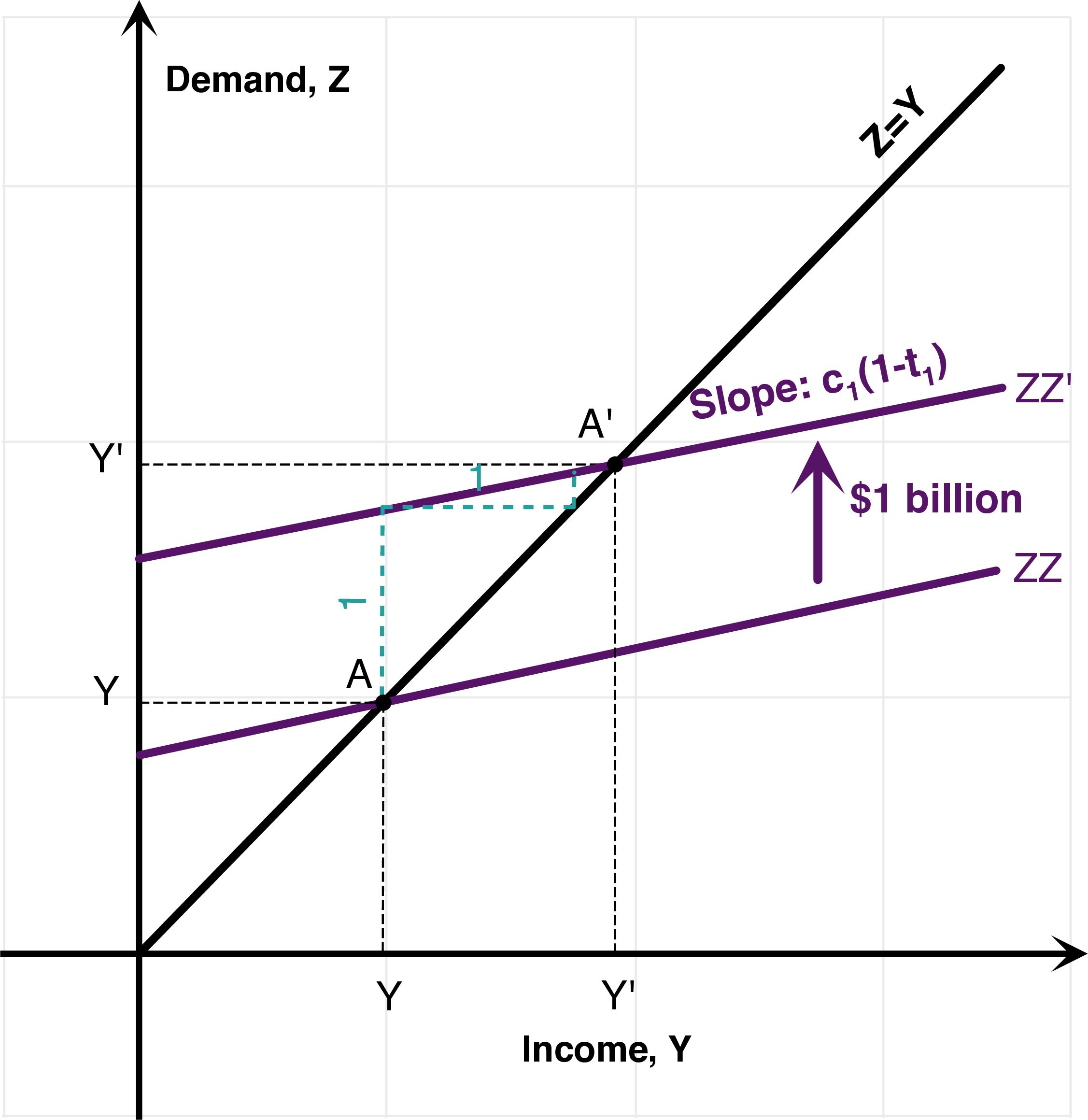
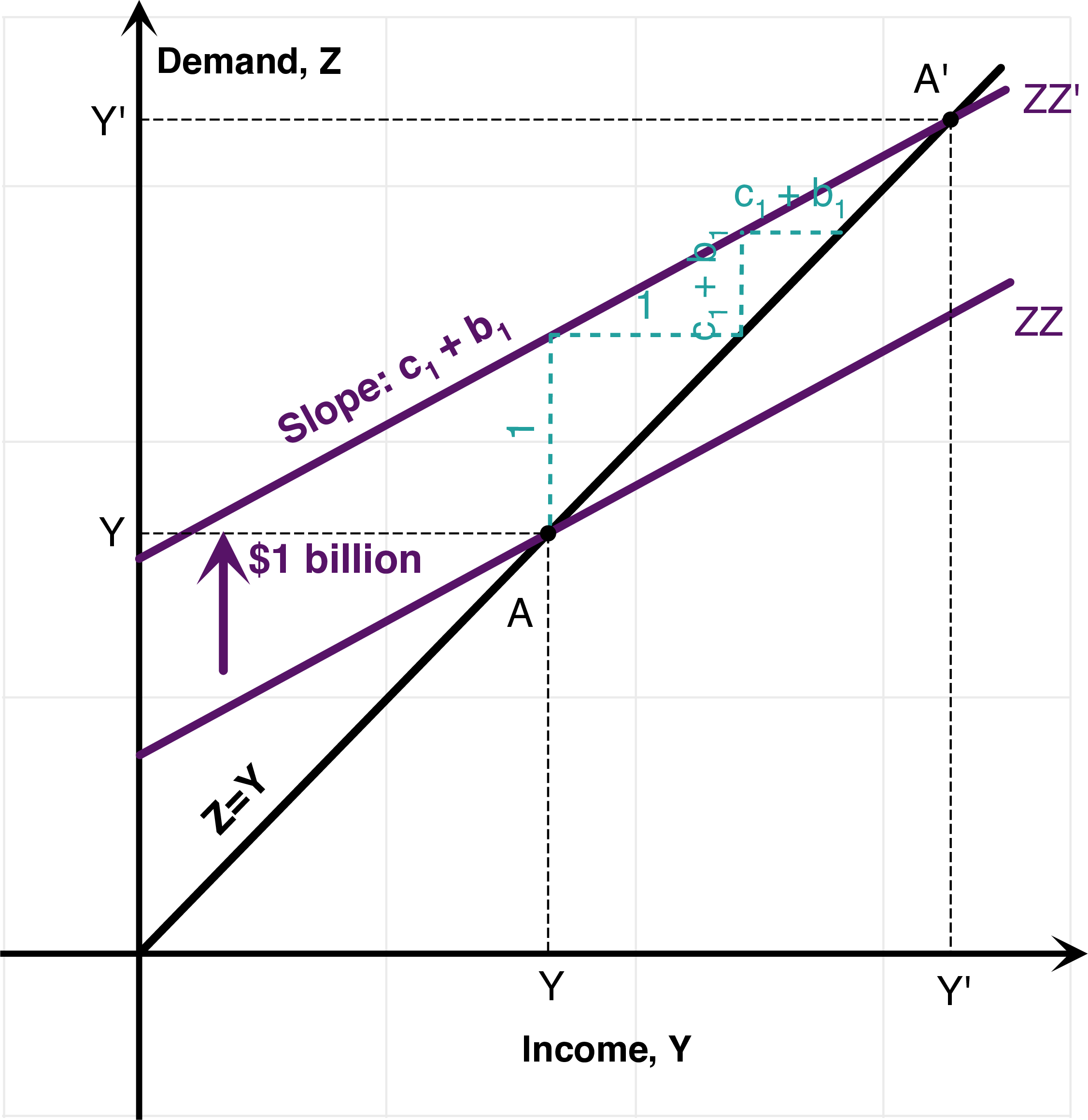
Figure 7.3: Variations: Automatic Stabilizers, Accelerator Effect.
7.4 “Accelerator” Effect
Another variation on the Goods Market model consists in recognizing that investment demand might also depend on income. Firms will invest more if they expect high income, and therefore high demand for their goods: \[I=b_{0}+b_{1}Y.\] Thus, the (ZZ)-curve now has a slope equal to \(c_1+b_1\): \[ \begin{aligned} Z &=C+I+G\\ &=c_{0}+c_{1}\left(Y-T\right)+b_{0}+b_{1}Y+G\\ Z &=\left(c_{0}-c_{1}T+b_{0}+G\right)+\left(c_{1}+b_{1}\right)Y. \end{aligned} \] Using \(Z=Y\), we can conclude that the multiplier is \(1/(1-c_1-b_1)\) if \(c_{1}+b_{1}<1\): \[Y=\frac{1}{1-\left(c_{1}+b_{1}\right)}\left(c_{0}-c_{1}T+b_{0}+G\right)\] In this case, the (ZZ) curve is steeper, and thus the multiplier \(Y'-Y\) is larger. Note that if \(c_{1}+b_{1}\geq1\), then the multiplier is infinite. This, of course, shows the limits of the Keynesian model: it remains valid as long as output is constrained by aggregate demand. In this case, output will increase to a level such as it becomes constrained by supply, as in lecture 1.5.
Required Readings
Robert Barro. Keynes Is Still Dead. Wall Street Journal. October 29, 1992.
Mankiw, N. Gregory. What would Keynes have done? New York Times, November 30, 2008
Robert J. Barro, Government Spending Is No Free Lunch, Wall Street Journal, January 22, 2009.
Bruce Bartlett. Keynes Was Really A Conservative. Forbes. August 14, 2009.