3 Capital Accumulation

Link to slides / Link to handouts

What are the sources of GDP growth, and of GDP differences across countries? As a matter of pure accounting, the supply-side approach to GDP presented in lecture 1, with GDP given as \(Y_t = A_t K_t^{\alpha} L_t^{1-\alpha},\) implies that growth in GDP may arise from technology, capital, or population. Population is natural, and probably not that interesting from an economist’s point of view, since the object of interest for an economist usually is GDP per capita – even though population is very important for discussions of relative economic or military power, which ultimately also impact the economy. So we are left with two factors of potential interest: capital accumulation, and technology growth. In this lecture, we study the Solow / Swan model of economic growth, which deals with the problem of capital accumulation.¹²

In the first four sections, we look at some data on saving (Section 3.1), the capital stock (Section 3.2), investment (Section 3.3), and depreciation (Section 3.4).

We then move on to study two versions of the Solow growth model. Section 3.5 considers the case of a Solow growth model with a constant returns to scale production function. Section 3.6 looks at a special case of the Solow growth model for a case of a Cobb-Douglas production function.

3.1 Data on Saving

Saving and Investment. Figure 3.1 plots gross saving and investment in the United States from the World Development Indicators put together by the World Bank. Figure 3.2 plots net saving and gross saving for the U.S.: net saving (gross saving net of depreciation) is slightly higher than 0, but not by much.

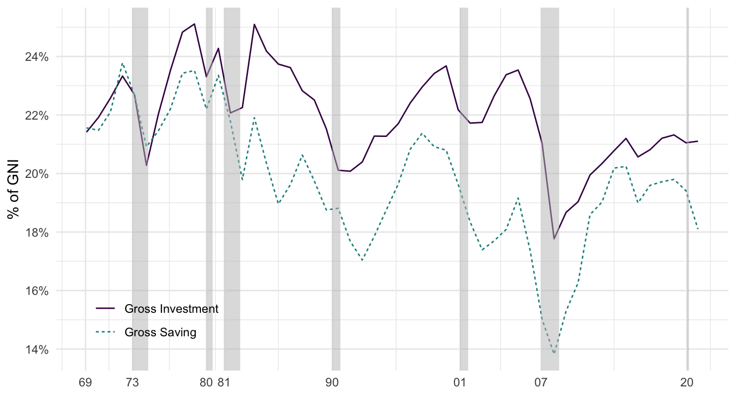
Figure 3.1: Gross Savings and Investment in the U.S. (WDI).

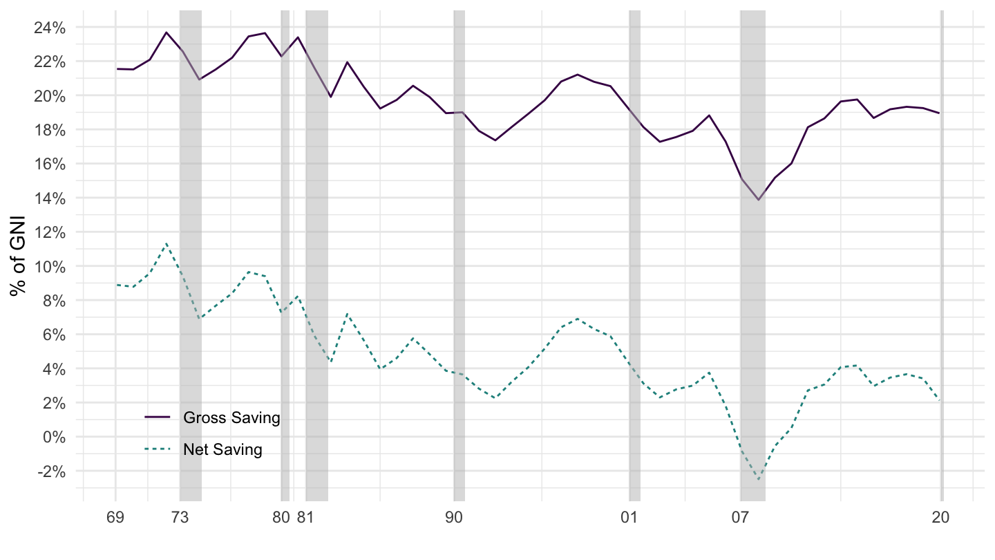
Figure 3.2: Net Savings and Gross savings (WDI).

Figure 3.3 plots gross saving as a % of GDP.

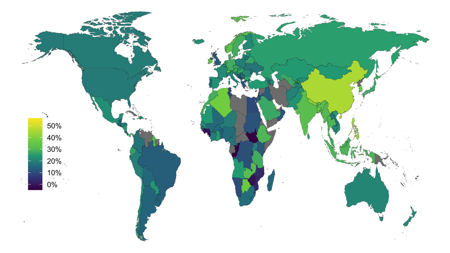
Figure 3.3: Gross Saving (% of GDP), 2016.

3.2 Data on Capital

What is Capital? Table 3.1 shows some data concerning capital, available from the BEA. This data is constructed using what is called the Perpetual Inventory Method (PIM): flows of investment are added, and depreciation is taken into account, in order to compute an aggregate capital stock. Two facts should be noted:

1. The Capital Stock is mostly comprised of buildings (residential and structures): in 2017, non-residential private structures are approximately 58.5% of GDP, residential fixed assets are 87.1% (this does not include land), and government structures 48.1% of GDP.

2. Private Equipment is only 27.5% of GDP in the private sector, and 4.2% of GDP in the government sector, totalling less than one third of GDP, or less than 15% of total fixed assets.

Table 3.1: What is Capital? (% of GDP) Source: Fixed Asset Table 1.1 (BEA)

Description	2017
Fixed assets and consumer durable goods	268%
Fixed assets	246.1%
Private	187%
Nonresidential	99.9%
Equipment	27.5%
Structures	58.9%
IPP	13.5%
Residential	87.1%
Government	59.1%
Nonresidential	57.4%
Equipment	4.2%
Structures	48.3%
IPP	4.9%
Residential	1.8%
Consumer durable goods	21.8%

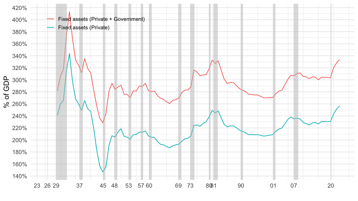
Figure 3.4: U.S. Main Fixed Asset Components (1929-2017). Source: Fixed Asset Table 1.1 (BEA)

Figure 3.5 shows the evolution of the main fixed asset components from the Fixed Asset Tables of the Bureau of Economic Analysis, over the period from 1929 to 2017.

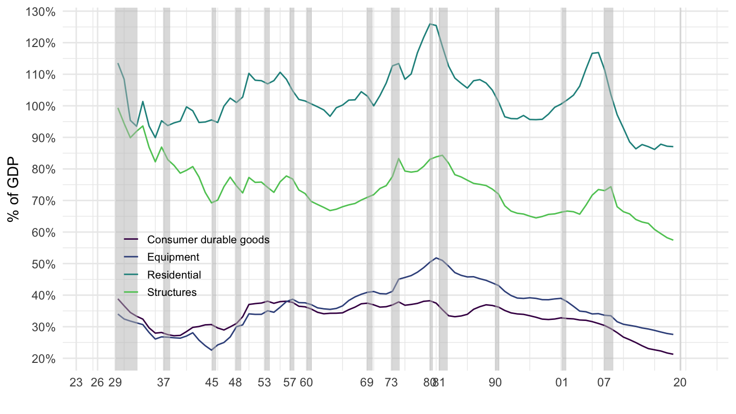
Figure 3.5: U.S. Main Fixed Asset Components (1929-2017). Source: Fixed Asset Table 1.1 (BEA)

What is Private Equipment? Given the potential importance of private equipment for macroeconomics, and in particular the role it plays in neoclassical theory as an “absorber” of saving flows, we shall now more into what equipment is. In particular, an important question will be how much we think it actually can be a substitute for labor in production. Table 3.2 shows some data concerning private equipment, available from the BEA. Figure 3.6 shows the evolution of the main private equipment components from the Fixed Asset Tables of the Bureau of Economic Analysis, over the period from 1929 to 2017.

Table 3.2: Decomposition of Equipment (% of GDP). Source: Fixed Asset Table 2.1 (BEA)

Description	2017
Private fixed assets	187%
Structures	145.8%
Nonresidential structures	58.9%
Commercial & health care	21.3%
Office	8%
Health care	4.5%
Hospitals & special care	3.5%
Hospitals	2.9%
Special care	0.6%
Medical buildings	0.9%
Multimerchandise shopping	3.1%
Food & beverage establishments	1.4%
Warehouses	2%
Other commercial	2.3%
Manufacturing	6.7%
Power & communication	11.3%
Power	8.7%
Electric	6.3%
Other power	2.4%
Communication	2.7%
Mining exploration, shafts, & wells	7.3%
Petroleum & natural gas	6.7%
Mining	0.6%
Other structures	12.3%
Religious	1.4%
Educational & vocational	2.3%
Lodging	2.7%
Amusement & recreation	1.6%
Transportion	2%
Air	0.2%
Land	1.8%
Farm	1.6%
Other	0.7%
Residential structures	86.9%
Housing units	65.7%
Permanent site	64.6%
1 to 4 unit	55.4%

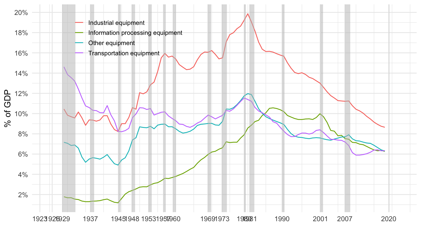
Figure 3.6: Decomposition of Equipment (% of GDP). Source: Fixed Asset Table 2.1 (BEA)

Decomposition of structures. Table 3.3 similarly breaks down structures into its different components.

Table 3.3: Decomposition of Structures (% of GDP). Source: Fixed Asset Table 2.1 (BEA)

Description	2017
Private fixed assets	187%
Structures	145.8%
Nonresidential structures	58.9%
Commercial & health care	21.3%
Office	8%
Health care	4.5%
Hospitals & special care	3.5%
Hospitals	2.9%
Special care	0.6%
Medical buildings	0.9%
Multimerchandise shopping	3.1%
Food & beverage establishments	1.4%
Warehouses	2%
Other commercial	2.3%
Manufacturing	6.7%
Power & communication	11.3%
Power	8.7%
Electric	6.3%
Other power	2.4%
Communication	2.7%
Mining exploration, shafts, & wells	7.3%
Petroleum & natural gas	6.7%
Mining	0.6%
Other structures	12.3%
Religious	1.4%
Educational & vocational	2.3%
Lodging	2.7%
Amusement & recreation	1.6%
Transportion	2%
Air	0.2%
Land	1.8%
Farm	1.6%
Other	0.7%
Residential structures	86.9%
Housing units	65.7%
Permanent site	64.6%
1 to 4 unit	55.4%
5-or more-unit	9.3%
Manufactured homes	1%
Brokers’ commissions	1.2%
Improvements	19.7%
Other residential	0.4%

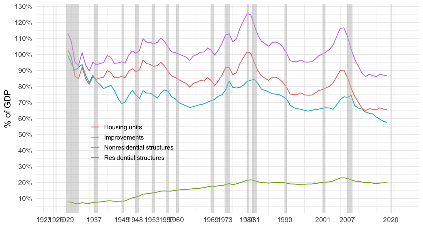
Figure 3.7: Decomposition of Structures (% of GDP). Source: Fixed Asset Table 2.1 (BEA)

3.3 Data on Investment

Figure 3.8 plots private and total net investment in the U.S., taking a longer term perspective, using the data in Piketty and Zucman (2016).¹³

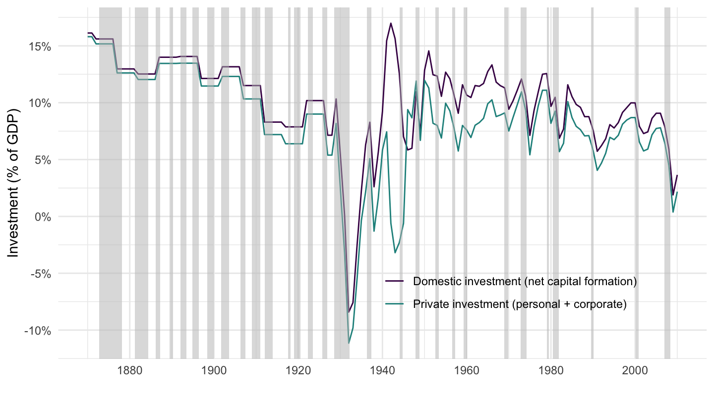
Figure 3.8: U.S. Private and Total Net Investment

Figure 3.9 plots investment as a % of GDP on a map of the world, while figure 3.3 plots gross saving as a % of GDP.

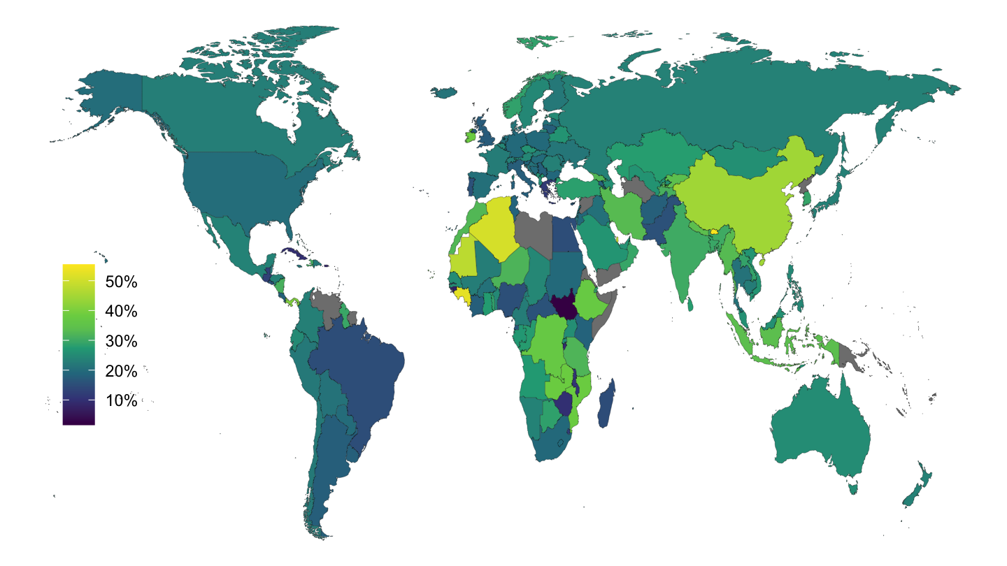
Figure 3.9: Investment (% of GDP), 2016.

What is Investment? Table 3.4 shows some data concerning investment, available from the BEA.

Table 3.4: What is Investment? (% of GDP) Source: Fixed Asset Table 1.5 (BEA)

Description	2017
Fixed assets and consumer durable goods	21.7%
Fixed assets	16.3%
Private	13.6%
Nonresidential	10.5%
Equipment	4.6%
Structures	2.3%
IPP	3.5%
Residential	3.1%
Government	2.7%
Nonresidential	2.7%
Equipment	0.6%
Structures	1.3%
IPP	0.8%
Residential	0%
Consumer durable goods	5.4%

Figure 3.10 shows the breakdown between private and government investment in the U.S., from the BEA. The impact of the Second World War should be very clear.

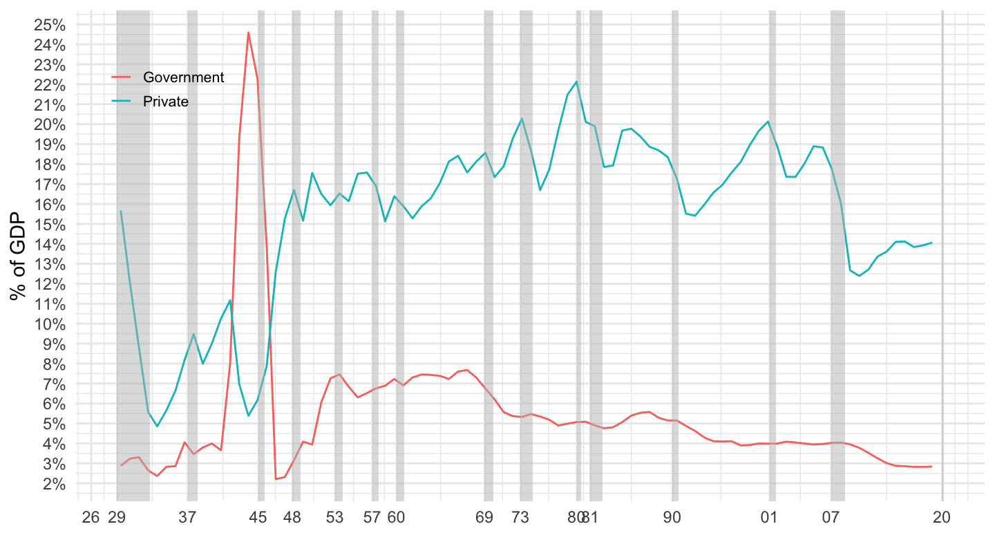
Figure 3.10: U.S. Investment, Government VS Private (% of GDP) Source: Fixed Asset Table 1.5 (BEA)

Figure 3.11 shows the evolution of the main private investment components in the U.S., over the period from 1929 to 2017.

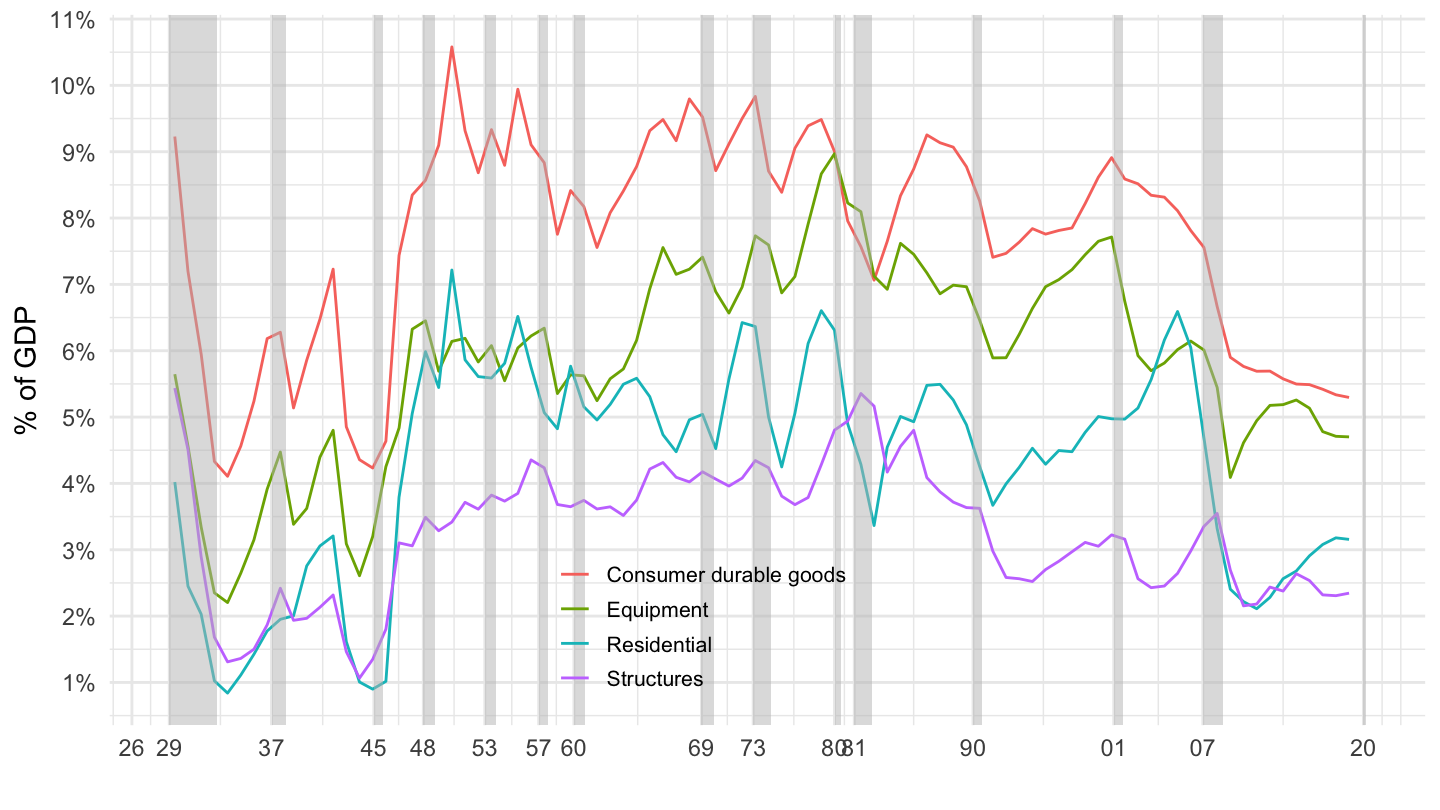
Figure 3.11: U.S. Private Investment, Main Components (% of GDP) Source: Fixed Asset Table 1.5 (BEA)

What is Private Equipment Investment? Again, we focus here on private equipment investment. Table 3.5 shows some data concerning private equipment, available from the BEA.

Table 3.5: Decomposition of Equipment Investment (% of GDP). Source: Fixed Asset Table 2.7 (BEA)

Description	2017
Private fixed assets	13.6%
Equipment	4.7%
Nonresidential equipment	4.6%
Information processing equipment	1.5%
Computers & peripheral equipment	0.4%
Communication equipment	0.5%
Medical equipment & instruments	0.4%
Nonmedical instruments	0.2%
Photocopy & related equipment	0%
Office & accounting equipment	0%
Industrial equipment	0.9%
Fabricated metal products	0.1%
Engines & turbines	0.1%
Metalworking machinery	0.1%
Special industry machinery, n.e.c.	0.2%
Gen. industrial, incl. materials handling, equip.	0.3%
Electrical transmission, distrib., & ind. apparatus	0.2%
Transportation equipment	1.1%
Trucks, buses, & truck trailers	0.7%
Light trucks (including utility vehicles)	0.5%
Other trucks, buses, & truck trailers	0.2%
Autos	0.1%
Aircraft	0.2%
Ships & boats	0%
Railroad equipment	0%
Other equipment	1%
Furniture & fixtures	0.2%
Agricultural machinery	0.1%
Construction machinery	0.2%
Mining & oilfield machinery	0.1%
Service industry machinery	0.2%
Electrical equipment, n.e.c.	0%
Other nonresidential equipment	0.2%
Residential equipment	0.1%

Figure 3.12 shows the evolution of the main private equipment investment components from the Fixed Asset Tables of the Bureau of Economic Analysis, over the period from 1929 to 2017.

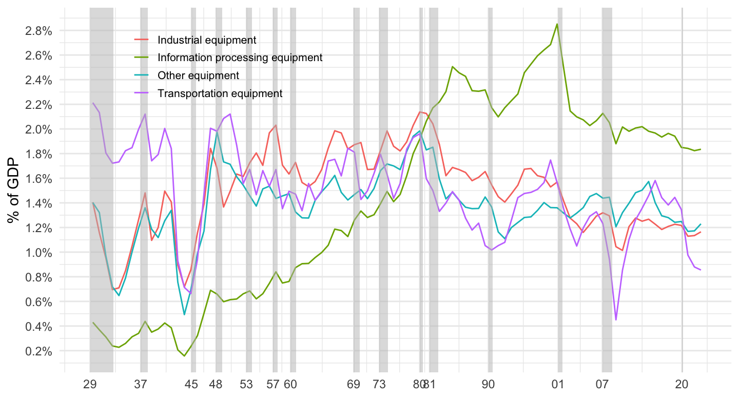
Figure 3.12: Decomposition of Equipment Investment (% of GDP). Source: Fixed Asset Table 2.7 (BEA)

3.4 Data on Depreciation

Table 3.6: What is Investment? (% of GDP) Source: Fixed Asset Table 1.3 (BEA)

Description	2017
Fixed assets and consumer durable goods	17.2%
Fixed assets	12.8%
Private	10.6%
Nonresidential	8.6%
Equipment	3.7%
Structures	1.8%
IPP	3.1%
Residential	2%
Government	2.2%
Nonresidential	2.2%
Equipment	0.5%
Structures	0.9%
IPP	0.8%
Residential	0%
Consumer durable goods	4.4%

Figure 3.13 shows the breakdown between private and government depreciation in the U.S., from the BEA.

Figure 3.13: U.S. Depreciation, Government VS Private (% of GDP) Source: Fixed Asset Table 1.3 (BEA)

Figure 3.14 shows the evolution of the main private depreciation components in the U.S., over the period from 1929 to 2017.

Figure 3.14: U.S. Private Depreciation, Main Components (% of GDP) Source: Fixed Asset Table 1.3 (BEA)

3.5 The Solow Growth Model

In this chapter, I present the Solow growth model.

Production function. Robert Solow, starts from a general production function, giving at any point in time output at time \(t\) \(Y_t\) as a function of \(2\) inputs, capital at time \(t\) \(K_t\) and labor at time \(t\) \(L_t\): \[Y_t=F\left(K_t,L_t\right).\] In terms of the Cobb-Douglas production function we saw in the previous lecture, the fact that \(F(.,.)\) does not depend on time implies that total factor productivity \(A_t\) is a constant. (there is no technological growth)¹⁴

Robert Solow further assumes constant returns to scale with respect to capital and labor, so that for any scaling factor \(a\): \[F(aK_t, aL_t) = aF(K_t, L_t).\] For example, for \(a=2\), when the quantity of labor and the quantity of capital are doubled, then we get double the quantity of output.¹⁵

Because of constant returns to scale, everything “scales with population”. For simplicity, we shall assume from now on that the quantity of labor is fixed with \(L_t=L\), so that the production function becomes \(Y_t=F(K_t, L)\).¹⁶

Because of constant returns to scale with respect to capital and labor (and setting \(a=1/L\) in the previous expression), we can express everything as a function of output per worker \(Y_t/L\) and capital per worker \(K_t/L\): \[\frac{Y_t}{L}=F\left(\frac{K_t}{L},1\right)=f\left(\frac{K_t}{L}\right),\] where \(f\) is defined as a function of \(F\) such that: \[f(x)\equiv F(x,1).\] An example of such a production function is the Cobb-Douglas production function, which we started studying in lecture 1, and which we look at in section 3.6.

Saving and Investment. Robert Solow, in his 1956 contribution, abstracts from public saving, so that total saving at time \(t\) equals private saving at time \(t\), and both are denoted \(S_{t}\), which also equals investment \(I_{t}\) at time \(t\) : \[S_{t}=I_{t}.\]

Saving is assumed to be a constant fraction \(s\) of output \(Y_{t}\), and therefore: \[S_{t}=sY_{t}.\]

This constant saving rate my seem a bit ad-hoc; it is. We will investigate more in detail the determinants of saving and consumption behavior in lecture 3. This implies that: \[\boxed{I_t = S_t = sY_t}.\]

Law of motion for capital. Depreciation of capital is given by a share \(\delta\). Think for example that 8% of the capital stock depreciates each period; the rate of depreciation is much lower for structures, and much higher for computers. The capital stock evolves according to: \[\boxed{K_{t+1}=\left(1-\delta\right)K_{t}+I_{t}}.\]

Law of motion for capital per worker. The law of motion for capital, together with the constant saving rate, implies: \[K_{t+1}=\left(1-\delta\right)K_{t}+sY_t.\]

Dividing both sides by \(L\) to scale everything by the number of worker (so that we are looking at capital per worker, as well as output per worker): \[\frac{K_{t+1}}{L} =\left(1-\delta\right)\frac{K_{t}}{L}+s\frac{Y_{t}}{L}\quad\Rightarrow\quad\boxed{\frac{K_{t+1}}{L}-\frac{K_{t}}{L}=s\frac{Y_{t}}{L}-\delta\frac{K_{t}}{L}}.\]

The change in the capital stock per worker from \(t\) to \(t+1\) has two components:

• investment per worker (equivalently, saving per worker) \(s Y_t / L\).
• depreciation per worker \(\delta K_t / L\).

Therefore, the law of motion for capital per worker is: \[\underbrace{\frac{K_{t+1}}{L}-\frac{K_{t}}{L}}_{\text{Change in capital }}=\underbrace{sf\left(\frac{K_{t}}{L}\right)}_{\text{Investment}}-\underbrace{\delta\frac{K_{t}}{L}}_{\text{Depreciation}}.\]

Steady-state. The steady state level of the capital stock \(K^{*}\) is such that \(K_{t+1}=K_{t}=K^{*}\), and it therefore satisfies: \[\boxed{sf\left(\frac{K^{*}}{L}\right)=\delta\frac{K^{*}}{L}}.\]

Note that without further specifying \(f(.)\), we can’t say much more about the value of \(K^{*}/L\), we just know it satisfies this implicit equation. The steady-state value of output per worker \(Y^{*}/L\), as a function of \(K^{*}/L\) is given by: \[\frac{Y^{*}}{L}=f\left(\frac{K^{*}}{L}\right).\]

Convergence to the steady-state. Without further specifying the shape of the production function, we may identify three cases. In all cases, there is convergence to the steady-state level of capital per worker \(K^{*}/L\) which was identified in the previous section.

1. If capital per worker is initially relatively low, that is \(K_{t}/L<K^{*}/L\), then investment per worker is larger than depreciation per worker, and therefore from the above equation, capital per worker increases: \[\boxed{\frac{K_t}{L}<\frac{K^{*}}{L} \quad \Rightarrow \quad \frac{K_{t+1}}{L}>\frac{K_{t}}{L}}.\]

2. If capital per worker is exactly equal to steady state capital per worker, that is \(K_{t}/L=K^{*}/L\), then investment per worker is equal to depreciation per worker, and therefore from the above equation, capital per worker stays constant: \[\boxed{\frac{K_t}{L}=\frac{K^{*}}{L} \quad \Rightarrow \quad \frac{K_{t+1}}{L}=\frac{K_{t}}{L}=\frac{K^{*}}{L}}.\]

3. If capital per worker is relatively high, that is \(K_{t}/L>K^{*}/L\), then depreciation per worker is larger than investment per worker, and therefore, capital per worker declines: \[\boxed{\frac{K_t}{L}>\frac{K^{*}}{L} \quad \Rightarrow \quad \frac{K_{t+1}}{L}<\frac{K_{t}}{L}}.\]

3.6 Cobb-Douglas production function

Production function. Assume now that the production function is a Cobb-Douglas production function, so that:
\[F(K,L)=K^{\alpha}L^{1-\alpha}.\] As we saw in the previous chapter, \(\alpha\) should be thought of as roughly equal to \(1/3\). This implies then that function \(f\) defined above is such that: \[f(x)=x^{\alpha}.\]

Law of motion for capital. The law of motion for capital is given by:
\[\frac{K_{t+1}}{L}=\frac{K_{t}}{L}+s\left(\frac{K_{t}}{L}\right)^{\alpha}-\delta\frac{K_{t}}{L}.\]

Given \(L\), \(K_{0}\), \(\alpha\), \(s\), \(\delta\), we are able to calculate \(K_{1}\), \(K_{2}\), …, as well as \(K_{t}\) for any \(t\), by calculating the quantities of capital successively from the formula above. If you do so, you will notice that \(K_{t}\) converges to a steady state value \(K^{*}\). However, you do not need to perform an infinity of operations to get at this \(K^{*}\).

Steady-state. In the Cobb-Douglas case, there is a simpler way to get steady-state capital per worker: what was an implicit equation in section 3.5 can now be solved for explicitely. Capital per worker in steady-state \(K^{*}/L\) solves: \[s\left(\frac{K^{*}}{L}\right)^{\alpha}=\delta\frac{K^{*}}{L}\quad\Rightarrow\quad \boxed{\frac{K^{*}}{L}=\left(\frac{s}{\delta}\right)^{\frac{1}{1-\alpha}}}.\]

The steady-state level of output per worker is then: \[\boxed{\frac{Y^{*}}{L}=\left(\frac{s}{\delta}\right)^{\frac{\alpha}{1-\alpha}}}.\]

We are also able to compute the steady-state capital to output ratio \(K^{*}/Y^{*}\) from the Solow growth model: \[ \begin{aligned} \frac{K^{*}}{Y^{*}}&=\frac{K^{*}/L}{Y^{*}/L}\\ &=\left(\frac{s}{\delta}\right)^{\frac{1}{1-\alpha}} \left(\frac{s}{\delta}\right)^{-\frac{\alpha}{1-\alpha}} \\ \frac{K^{*}}{Y^{*}}&= \frac{s}{\delta}. \end{aligned} \] Alternatively, you may obtain this expression much more simply by equating saving \(sY^{*}\) to investment \(\delta K^{*}\) in the steady state: \[sY^{*} = \delta K^{*} \quad \Rightarrow \quad \boxed{\frac{K^{*}}{Y^{*}} = \frac{s}{\delta}}.\]

Another object of potential interest is the steady-state marginal product of capital (also called Rental Rate of capital \(R^{*}\), see lecture 1: \[ \begin{aligned} R^{*}&=\alpha \left(K^{*}\right)^{\alpha-1} L^{1-\alpha}\\ &=\alpha\left(\frac{K^{*}}{L}\right)^{\alpha-1}\\ &=\alpha\left(\frac{s}{\delta}\right)^{\frac{\alpha-1}{1-\alpha}}\\ R^{*}&=\frac{\alpha \delta}{s} \end{aligned} \] Therefore, the steady-state marginal product of capital is given by: \[\boxed{R^{*}=\frac{\alpha \delta}{s}}.\]

The steady-state net marginal product of capital \(r^{*}\), which is the gross marginal product of capital minus depreciation (relevant for calculating the real return to an investor) is thus given by: \[ \begin{aligned} r^{*}&=R^{*}-\delta\\ r^{*}&=\frac{\alpha \delta}{s}-\delta \end{aligned} \] Therefore, the steady-state net marginal product of capital is given by: \[\boxed{r^{*}=\frac{\alpha \delta}{s}-\delta}.\]

Finally, steady-state consumption per worker is given by: \[ \begin{aligned} \frac{C^{*}}{L}&=(1-s)\frac{Y^{*}}{L}\\ &=(1-s)\left(\frac{s}{\delta}\right)^{\frac{\alpha}{1-\alpha}}\\ \frac{C^{*}}{L}&=\frac{(1-s)s^{\frac{\alpha}{1-\alpha}}}{\delta^{\frac{\alpha}{1-\alpha}}} \end{aligned} \]

Thus, consumption per capita at the steady-state is: \[\boxed{\frac{C^{*}}{L}=\frac{(1-s)s^{\frac{\alpha}{1-\alpha}}}{\delta^{\frac{\alpha}{1-\alpha}}}}.\]

3.7 Golden Rule

Most economists believe that policymakers should not care so much about GDP per person, but rather about consumption per person (however, some people hold a different view - we shall talk about that later). The intuition is simple: if an economy was to produce many goods which were only used for investment purposes (which would be the case if \(s = 1\)), then people in this economy would be starving, even though it was actually producing a lot. Investment, ultimately, should serve to increase future consumption.

The Golden Rule level of capital accumulation is such that the level of steady-state consumption per capita is maximized. Again, from the previous section, steady-state consumption per capita is given by: \[ \begin{aligned} \frac{C^{*}}{L}=\frac{(1-s)s^{\frac{\alpha}{1-\alpha}}}{\delta^{\frac{\alpha}{1-\alpha}}}. \end{aligned} \]

Maximizing this steady state consumption with respect to the saving rate \(s\) consists in finding the maximum of that function with respect to \(s\): \[\frac{d\left(C^{*}/L\right)}{ds}=0\quad\Rightarrow\quad\frac{d\left[(1-s)s^{\frac{\alpha}{1-\alpha}}\right]}{ds}=0.\] Note that \(1/\delta^{\alpha/(1-\alpha)}\) is a constant which does not change anything to the maximization.¹⁷ The first order condition is therefore: \[-s^{\frac{\alpha}{1-\alpha}}+\frac{\alpha}{1-\alpha}(1-s)s^{\frac{\alpha}{1-\alpha}-1}=0.\]

Noting that we can divide by \(s^{\alpha/(1-\alpha)}\) and then doing some algebra allows to get at the Golden Rule saving rate: \[ \begin{aligned} &-1 + \frac{\alpha}{1-\alpha}(1-s)s^{-1}=0\\ &\quad \Rightarrow\quad\frac{\alpha}{1-\alpha}\frac{1-s}{s}=1\\ &\quad \Rightarrow \quad \alpha(1-s)=(1-\alpha)s\\ &\quad \Rightarrow\quad\alpha-\alpha s=s-\alpha s\\ &\quad\Rightarrow\quad\boxed{s=\alpha}. \end{aligned} \]

Therefore, the saving rate corresponding to the Golden Rule level of capital accumulation is equal to \(\alpha\) (again, taking \(\alpha\) to be equal to roughly 1/3, this would suggest that an economy would optimally need to save about a third of its production every year).

We can then use the expressions that were found in section ??, substituting out the saving rate \(s\) with \(\alpha\).

Capital per worker. The Golden Rule level of capital accumulation is then such that capital per worker at the steady-state is: \[\frac{K^{*}}{L}=\left(\frac{s}{\delta}\right)^{\frac{1}{1-\alpha}}\quad\Rightarrow_{s=\alpha}\quad \boxed{\frac{K^{*}_g}{L}=\left(\frac{\alpha}{\delta}\right)^{\frac{1}{1-\alpha}}}.\]

Output per worker. At the Golden Rule, steady-state GDP per worker is: \[\frac{Y^{*}}{L}=\left(\frac{s}{\delta}\right)^{\frac{\alpha}{1-\alpha}}\quad\Rightarrow_{s=\alpha}\quad \boxed{\frac{Y^{*}_g}{L}=\left(\frac{\alpha}{\delta}\right)^{\frac{\alpha}{1-\alpha}}}.\]

Capital-Output Ratio. At the Golden Rule, the steady-state capital to output ratio is: \[\frac{K^{*}}{Y^{*}} = \frac{s}{\delta} \quad \Rightarrow_{s=\alpha} \quad \boxed{\frac{K^{*}_g}{Y^{*}_g} = \frac{\alpha}{\delta}}.\]

MPK. At the Golden Rule, the steady-state Marginal Product of Capital is: \[ R^{*}=\frac{\alpha \delta}{s} \quad \Rightarrow_{s=\alpha} \quad \boxed{R^*_g = \delta}. \] Note: Another way to see that for the Golden Rule level of capital, the marginal product of capital \(R^{*}_g\) necessarily equals the rate of depreciation \(\delta\) is to note that maximizing consumption \(C^{*}\) is the same as maximizing output minus saving \((1-s)Y^{*} = Y^{*} - s Y^{*}\), and that saving in the steady-state equals depreciation in the steady-state (see above) so that \(s Y^{*}=\delta K^{*}\). Therefore, maximizing consumption \(C^{*}\) is maximizing \(Y^{*}-\delta K^{*}.\) But the derivative of that expression implies that: \[ \begin{aligned} &\frac{\partial C^{*}}{\partial K^{*}}=0 \quad \Rightarrow \quad \frac{\partial (Y^{*}-\delta K^{*})}{\partial K^{*}}=0\\ & \quad \Rightarrow \quad \frac{\partial Y^{*}}{\partial K^{*}}-\delta=0 \quad \Rightarrow \quad R^{*}_g=\delta. \end{aligned} \] Intuitively, at the steady-state optimum, the annual gain of an additional unit of capital, \(\partial Y^{*}/ \partial K^{*}\) in additional output, must equal the cost of paying the resulting annual maintainance cost \(\delta\) for this additional unit. If the marginal gain is higher than the marginal cost, then there is not enough capital. Should the marginal gain be lower than the marginal cost, then there would be too much capital. At the optimum, the marginal gain equals the marginal cost, so \(R^{*}_g=\delta.\)

Net MPK. At the Golden Rule, the steady-state net Marginal Product of Capital is: \[ r^{*}=\frac{\alpha \delta}{s}-\delta \quad \Rightarrow_{s=\alpha} \quad \boxed{r^*_g = 0}. \] Therefore, at the Golden Rule level of capital accumulation, the net marginal product of capital is equal to 0.
Note: Again, this should be obvious from the previous discussion on \(R^{*}_g\). Maximizing \(C^{*}\) is maximizing \(Y^{*}-\delta K^{*}\), and the derivative of this expression is equal to \(r^{*}\). Therefore, at the Golden Rule, the net return is equal to \(0\): \[\frac{\partial C^{*}}{\partial K^{*}}=0 \quad \Rightarrow \quad \frac{\partial Y^{*}}{\partial K^{*}}-\delta=0 \quad \Rightarrow \quad r^{*}_g=0.\]

Consumption per worker. Finally, at the Golden Rule, consumption per worker is: \[ \begin{aligned} \frac{C^{*}}{L}=\frac{(1-s)s^{\frac{\alpha}{1-\alpha}}}{\delta^{\frac{\alpha}{1-\alpha}}} \quad \Rightarrow_{s=\alpha} \quad \boxed{\frac{C^{*}_g}{L}=\frac{(1-\alpha)\alpha^{\frac{\alpha}{1-\alpha}}}{\delta^{\frac{\alpha}{1-\alpha}}}}. \end{aligned} \]

3.8 Taking Stock

What have we learnt from the Solow growth model? We have learned that to the extent that capital accumulation is useful for production (that is, output increases in the amount of accumulated capital), accumulated savings play a useful role, in that they allow to produce more output in the future.

At the same time, if consumption is the sole purpose of production, it does not make much sense to save too much all the time, either. In the limit, if all the output is always used to build new machines, then even though the economy is very productive, consumption is zero. The Golden Rule level of capital accumulation defines an optimal level of saving which allows to maximize steady-state consumption. With zero growth (of technology and population), this level of saving is such that the (net) rate of interest is exactly equal to zero \(r^*_g = 0\). In problem set 2, you will show that one can derive something analog for a case where there is productivity growth (\(A_t\) is growing) and population growth (\(L_t\) is growing).

Additional Readings

Humans 1, Robots 0, Wall Street Journal, October 6, 2013.

(Gated) Economists understand little about the causes of growth, The Economist, April 12, 2018.

---

12. Solow, Robert M. 1956. “A Contribution to the Theory of Economic Growth.” The Quarterly Journal of Economics 70 (1): 65–94. You can read the article here: https://doi.org/10.2307/1884513, but it is quite technical.↩

13. Piketty, Thomas, and Gabriel Zucman. 2014. “Capital Is Back: Wealth-Income Ratios in Rich Countries 17002010.” The Quarterly Journal of Economics 129 (3): 1255–1310. https://doi.org/10.1093/qje/qju018↩

14. This assumption shall be relaxed in Problem Set 2, where we shall consider technology growth. (as well as population growth)↩

15. This is sometimes called the replication argument. By replicating a factory with the same number of workers, and the same machines in them, then the new factory should be able to produce as much.↩

16. Again, this assumption shall be relaxed in Problem Set 2, where we shall consider population growth (on top of technology growth).↩

17. If you are not convinced that it is equivalent to maximize the function of \(s\) without the constant, then you may as well compute the derivative with respect to the whole \(C^{*}/L\) expression.↩