2 Consumption and Saving
Link to slides / Link to handouts
Consumption and saving are perhaps the most important and controversial issues in macroeconomics. In the Solow growth model, saving was a constant fraction \(s\) of GDP, by assumption. We now build on Economics 11 (the one where you learn consumer optimization with Lagrangians, and all of that), in order to derive saving behavior from microeconomic principles. In other words, we work to make saving “endogenous” (that is, explained by the model), while it was previously taken as exogenous (that is, assumed in the model).
Although this discussion may appear somewhat abstract at first, these calculations are the basis of some of the most important controversies in macroeconomics, which we shall come to in the next lectures.
2.1 Some data from the Consumer Expenditure Survey (CEX)
Before thinking about the theory of consumption, we first look at some data on consumption and saving coming from the Consumer Expenditure Survey (CEX).5
Main Components of Consumption. Table ?? presents data on total average annual expenditures of different income deciles: the first income decile (the first decile of the population), the middle income decile (the 5th decile of the population) and finally the high income decile (the last decile of the population). This table reads as follows: the low income decile spends on average $23588 every year, out of which $3789 on average is spent on food.
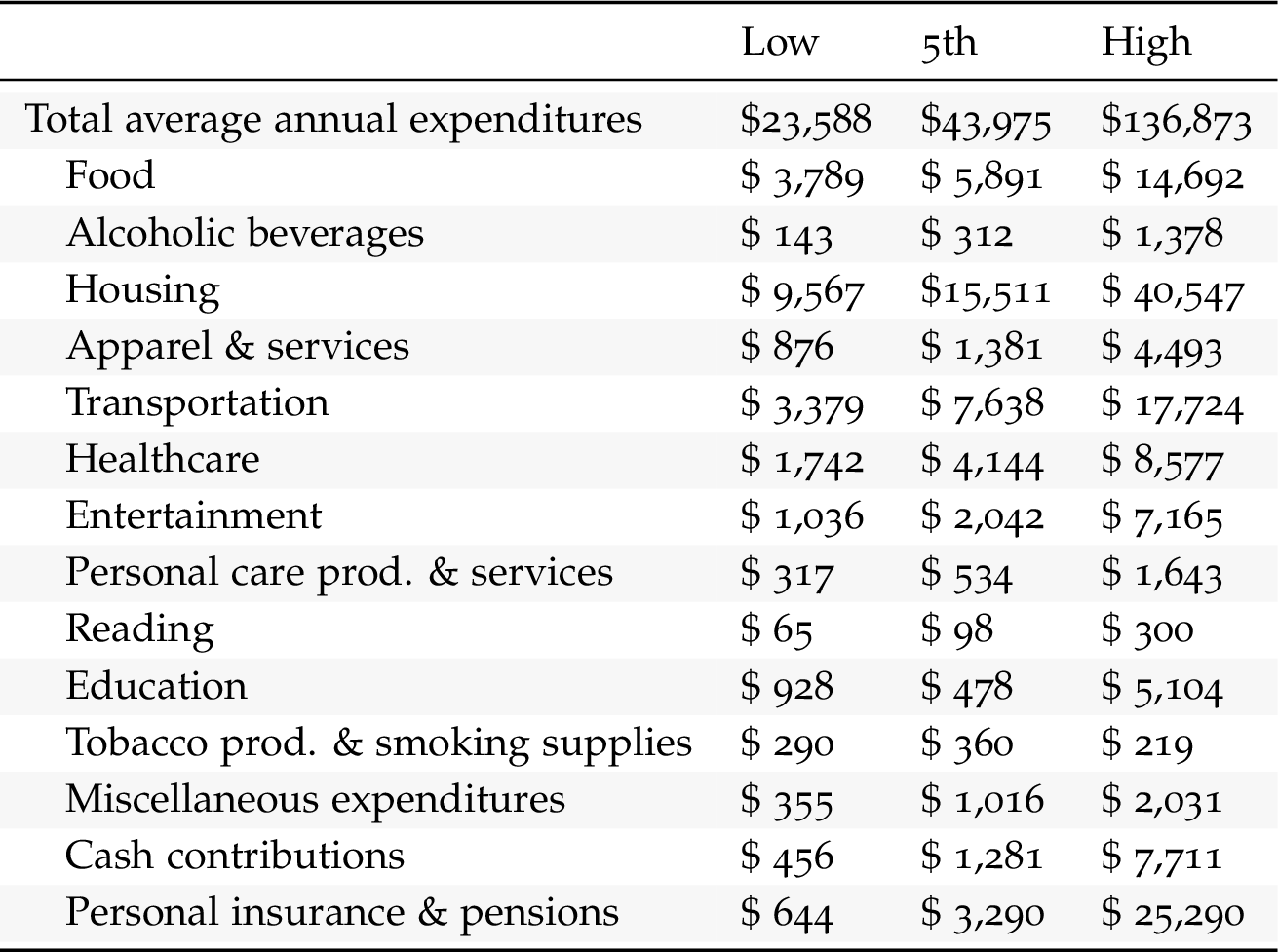
Table 2.1 shows the same data, but as a fraction of total average annual expenditures: for example, the lowest income decile spends 16.1% of its expenditures on food, while the high income decile spends only 10.7% of its expenditures on food.
| Low | 5th | High | |
|---|---|---|---|
| Total average annual expenditures | 100% | 100% | 100% |
| Food | 16.1% | 13.4% | 10.7% |
| Alcoholic beverages | 0.6% | 0.7% | 1% |
| Housing | 40.6% | 35.3% | 29.6% |
| Apparel & services | 3.7% | 3.1% | 3.3% |
| Transportation | 14.3% | 17.4% | 12.9% |
| Healthcare | 7.4% | 9.4% | 6.3% |
| Entertainment | 4.4% | 4.6% | 5.2% |
| Personal care prod. & services | 1.3% | 1.2% | 1.2% |
| Reading | 0.3% | 0.2% | 0.2% |
| Education | 3.9% | 1.1% | 3.7% |
| Tobacco prod. & smoking supplies | 1.2% | 0.8% | 0.2% |
| Miscellaneous expenditures | 1.5% | 2.3% | 1.5% |
| Cash contributions | 1.9% | 2.9% | 5.6% |
| Personal insurance & pensions | 2.7% | 7.5% | 18.5% |
Consumption by detailed category. Table 2.2 shows more detail, dividing up each category into more refined ones. For example, “food” is now divided between “food at home” and “food away from home”.
| Low | 5th | High | |
|---|---|---|---|
| Total average annual expenditures | $23,588 | $43,975 | $136,873 |
| Food | $ 3,789 | $ 5,891 | $ 14,692 |
| Food at home | $ 2,407 | $ 3,526 | $ 6,876 |
| Food away from home | $ 1,382 | $ 2,364 | $ 7,815 |
| Alcoholic beverages | $ 143 | $ 312 | $ 1,378 |
| Housing | $ 9,567 | $15,511 | $ 40,547 |
| Shelter | $ 5,873 | $ 8,966 | $ 24,593 |
| Utilities, fuels, & public services | $ 2,121 | $ 3,665 | $ 6,097 |
| Household operations | $ 547 | $ 923 | $ 3,962 |
| Housekeeping supplies | $ 388 | $ 582 | $ 1,208 |
| Household furnishings & equip. | $ 638 | $ 1,374 | $ 4,686 |
| Apparel & services | $ 876 | $ 1,381 | $ 4,493 |
| Apparel, Men & boys | $ 261 | $ 298 | $ 1,032 |
| Apparel, Women & girls | $ 351 | $ 537 | $ 1,486 |
| Apparel, Children under 2 | $ 14 | $ 33 | $ 118 |
| Footwear | $ 139 | $ 352 | $ 873 |
| Other apparel products & services | $ 111 | $ 160 | $ 985 |
| Transportation | $ 3,379 | $ 7,638 | $ 17,724 |
| Vehicle purchases (net outlay) | $ 1,139 | $ 3,124 | $ 6,797 |
| Gasoline, other fuels, & motor oil | $ 835 | $ 1,815 | $ 2,931 |
| Other vehicle expenses | $ 1,203 | $ 2,374 | $ 5,621 |
| Public & other transportation | $ 202 | $ 324 | $ 2,374 |
| Healthcare | $ 1,742 | $ 4,144 | $ 8,577 |
| Health insurance | $ 1,210 | $ 2,922 | $ 5,614 |
| Medical services | $ 255 | $ 664 | $ 1,899 |
| Drugs | $ 226 | $ 450 | $ 718 |
| Medical supplies | $ 51 | $ 107 | $ 345 |
| Entertainment | $ 1,036 | $ 2,042 | $ 7,165 |
| Entertainment: fees & admissions | $ 140 | $ 300 | $ 2,633 |
| Audio & visual equip. & services | $ 552 | $ 993 | $ 1,832 |
| Pets, toys, & playground equip. | $ 275 | $ 561 | $ 1,642 |
| Entertainment: other | $ 68 | $ 188 | $ 1,057 |
| Personal care products & services | $ 317 | $ 534 | $ 1,643 |
| Reading | $ 65 | $ 98 | $ 300 |
| Education | $ 928 | $ 478 | $ 5,104 |
| Tobacco products & smoking supplies | $ 290 | $ 360 | $ 219 |
| Miscellaneous expenditures | $ 355 | $ 1,016 | $ 2,031 |
| Cash contributions | $ 456 | $ 1,281 | $ 7,711 |
| Personal insurance & pensions | $ 644 | $ 3,290 | $ 25,290 |
| Life & other personal insurance | $ 76 | $ 216 | $ 1,014 |
| Pensions & Social Security | $ 568 | $ 3,074 | $ 24,276 |
Table 2.3 again presents this same data in as a fraction of total average annual expenditures. Perhaps unsurprisingly, “food away from home” is roughly a constant fraction of total average annual expenditures, implying that richer people either eat out more often, or do so in more expensive restaurants, while “food at home” in contrast is a declining share of annual expenditures as income rises: rich or poor, there’s only so much one can eat.
| Low | 5th | High | |
|---|---|---|---|
| Total average annual expenditures | 100% | 100% | 100% |
| Food | 16.1% | 13.4% | 10.7% |
| Food at home | 10.2% | 8% | 5% |
| Food away from home | 5.9% | 5.4% | 5.7% |
| Alcoholic beverages | 0.6% | 0.7% | 1% |
| Housing | 40.6% | 35.3% | 29.6% |
| Shelter | 24.9% | 20.4% | 18% |
| Utilities, fuels, & public services | 9% | 8.3% | 4.5% |
| Household operations | 2.3% | 2.1% | 2.9% |
| Housekeeping supplies | 1.6% | 1.3% | 0.9% |
| Household furnishings & equip. | 2.7% | 3.1% | 3.4% |
| Apparel & services | 3.7% | 3.1% | 3.3% |
| Apparel, Men & boys | 1.1% | 0.7% | 0.8% |
| Apparel, Women & girls | 1.5% | 1.2% | 1.1% |
| Apparel, Children under 2 | 0.1% | 0.1% | 0.1% |
| Footwear | 0.6% | 0.8% | 0.6% |
| Other apparel prod. & services | 0.5% | 0.4% | 0.7% |
| Transportation | 14.3% | 17.4% | 12.9% |
| Vehicle purchases (net outlay) | 4.8% | 7.1% | 5% |
| Gasoline, other fuels, & motor oil | 3.5% | 4.1% | 2.1% |
| Other vehicle expenses | 5.1% | 5.4% | 4.1% |
| Public & other transportation | 0.9% | 0.7% | 1.7% |
| Healthcare | 7.4% | 9.4% | 6.3% |
| Health insurance | 5.1% | 6.6% | 4.1% |
| Medical services | 1.1% | 1.5% | 1.4% |
| Drugs | 1% | 1% | 0.5% |
| Medical supplies | 0.2% | 0.2% | 0.3% |
| Entertainment | 4.4% | 4.6% | 5.2% |
| Entertainment: fees & admissions | 0.6% | 0.7% | 1.9% |
| Audio & visual equip. & services | 2.3% | 2.3% | 1.3% |
| Pets, toys, & playground equip. | 1.2% | 1.3% | 1.2% |
| Entertainment: other | 0.3% | 0.4% | 0.8% |
| Personal care prod. & services | 1.3% | 1.2% | 1.2% |
| Reading | 0.3% | 0.2% | 0.2% |
| Education | 3.9% | 1.1% | 3.7% |
| Tobacco prod. & smoking supplies | 1.2% | 0.8% | 0.2% |
| Miscellaneous expenditures | 1.5% | 2.3% | 1.5% |
| Cash contributions | 1.9% | 2.9% | 5.6% |
| Personal insurance & pensions | 2.7% | 7.5% | 18.5% |
| Life & other personal insurance | 0.3% | 0.5% | 0.7% |
| Pensions & Social Security | 2.4% | 7% | 17.7% |
Saving by income class. The above categories break down the average annual expenditures among different types. An interesting variable to look at also is how much people save. Figure 2.1 shows the saving rate by wealth class, again coming from the Consumer Expenditure Survey: according to this data, the rich save substantially more than the poor. It should be noted moreover that this is an understatement of the phenomenon: indeed, as the previous table showed, the top decile “spends” about 17.7% of their expenditures in “Pensions and Social Security”, a substantial part of it really can be considered as saving. In contrast, the bottom deciles spends only 2.4%.
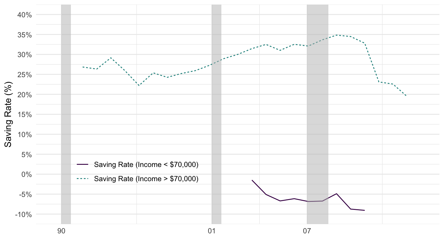
Figure 2.1: Saving by Income Class. Source: CEX
Figures 2.2, 2.3 and 2.4 are from Emmanuel Saez and Gabriel Zucman’s “Wealth Inequality in the United States since 1913: Evidence from Capitalized Income Tax Data,” published in 2016 in The Quarterly Journal of Economics.6 Figure 2.2 shows that the rich save much more than the poor, as a fraction of their incomes.
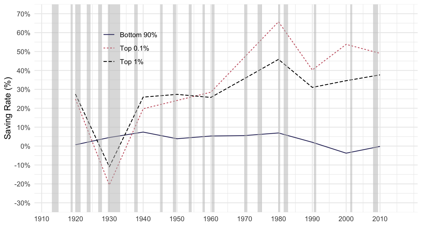
Figure 2.2: Saving by Wealth Class. Source: Saez, Zucman (2016)
Figure 2.3 shows the top 10% wealth share. As you can see, nearly 75% of household wealth is held by the top 10% wealth owners. This is more concentrated than labor income (the top 10% in the United States gets about 50% of pre-tax income, and much less after-tax), and therefore does not appear to be solely accounted for by saving for retirement.
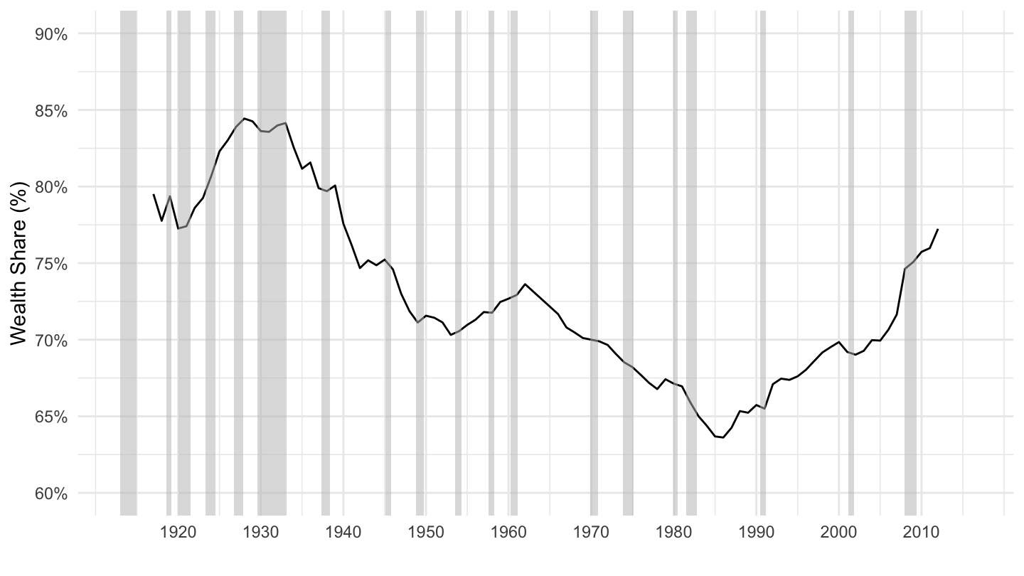
Figure 2.3: Top 10% wealth share. Source: Saez, Zucman (2016)
Figure 2.4 shows the top 1% wealth share, and the top 1-10% wealth share. As you can see, the top 1% now owns nearly 40% of the wealth in the United States, while it only accounts for about 20-25% of pre-tax income. Again, it does not seem like saving for retirement is the whole story.
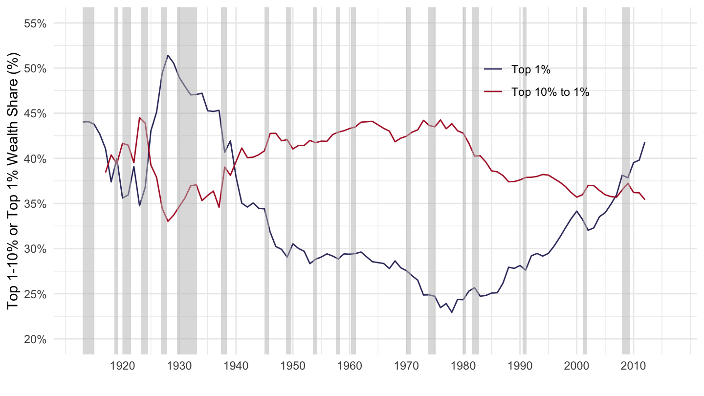
Figure 2.4: Top 1-10% and Top 1% wealth share. Source: Saez, Zucman (2016)
Table 2.4 shows some data concerning expenditures and saving of the top two deciles. It should be noted that both “personal insurance and pensions”, and the difference between income after taxes and total expenditures can be considered as saving.
| 9th 10% | High 10% | |
|---|---|---|
| Total average annual expenditures | 80.4% | 66.6% |
| Food | 9.5% | 7.2% |
| Alcoholic beverages | 0.7% | 0.7% |
| Housing | 24.6% | 19.7% |
| Apparel and services | 2.3% | 2.2% |
| Transportation | 13.3% | 8.6% |
| Healthcare | 6.2% | 4.2% |
| Entertainment | 4.2% | 3.5% |
| Personal care prod. and services | 1% | 0.8% |
| Reading | 0.1% | 0.1% |
| Education | 1.9% | 2.5% |
| Tobacco prod. and smoking supplies | 0.4% | 0.1% |
| Miscellaneous expenditures | 1.3% | 1% |
| Cash contributions | 2.5% | 3.8% |
| Personal insurance and pensions | 12.2% | 12.3% |
| Income after taxes | 100% | 100% |
| 9th 10% | High 10% | |
|---|---|---|
| Total average annual expenditures | $ 87,432 | $136,873 |
| Food | $ 10,328 | $ 14,692 |
| Alcoholic beverages | $ 785 | $ 1,378 |
| Housing | $ 26,719 | $ 40,547 |
| Apparel and services | $ 2,526 | $ 4,493 |
| Transportation | $ 14,495 | $ 17,724 |
| Healthcare | $ 6,772 | $ 8,577 |
| Entertainment | $ 4,604 | $ 7,165 |
| Personal care prod. and services | $ 1,085 | $ 1,643 |
| Reading | $ 157 | $ 300 |
| Education | $ 2,097 | $ 5,104 |
| Tobacco prod. and smoking supplies | $ 386 | $ 219 |
| Miscellaneous expenditures | $ 1,462 | $ 2,031 |
| Cash contributions | $ 2,739 | $ 7,711 |
| Personal insurance and pensions | $ 13,278 | $ 25,290 |
| Income after taxes | $108,743 | $205,391 |
2.2 The Two-Period Consumption Problem
Assumptions. There are two periods, \(t=0\) (think of this as “today”) and \(t=1\) (think of this as “tomorrow”). The consumer values consumption \(c_0\) in period \(0\) and \(c_1\) in period \(1\) according to the following utility function:
\[U(c_{0},c_{1})=u(c_{0})+\beta u(c_{1}).\]
where \(u(.)\) is an increasing and concave function, and \(\beta \leq 1\). \(\beta\) captures that people typically have a preference for the present. (they are present-biased)
Assume that agents earn (labor) income \(y_{0}\) in period \(0\), and (labor) income \(y_{1}\) in period \(1\). They also are born with some financial wealth \(f_{0}\) now, and have financial wealth \(f_{1}\) in period 1, which they consume entirely because this is the last period. (there is no point keeping more money for after period 1, because there is no future at that point) The amount that agents save in this economy is thus \(f_{1}-f_{0}\), and the amount of their accumulated savings is the savings they already had plus what they decided to accumulate, so that \(f_{0}+(f_{1}-f_{0})=f_{1}.\)
Therefore, consumption in period \(0\) is given by:
\[c_{0} =y_{0}-(f_{1}-f_{0})\]
The second period consumption \((t=1)\) is given by income plus the return to (accumulated !) savings:
\[c_{1} =y_{1}+(1+r)f_{1}.\]
Constrained Optimization Problem. Here, we show that the previous problem can actually be written as a maximization problem, subject to a budget constraint. Rewriting \(f_{1}\) from this second equation: \(f_{1}=(c_{1}-y_{1})/(1+r)\), and plugging into the first,
\[c_{0}=y_{0}-\left(\frac{c_{1}-y_{1}}{1+r}-f_{0}\right).\] Rearranging, total wealth is then the sum of financial wealth \(f_0\) and of the present discounted value of human wealth:
\[c_{0}+\frac{c_{1}}{1+r}=\overbrace{f_{0}+\underbrace{y_{0}+\frac{y_{1}}{1+r}}_{\text{human wealth}}}^{\text{total wealth}}.\]
The intertemporal budget constraint says that the present discounted value of consumption is equal to total wealth.
Optimization. The problem of the consumer is then simply that of maximizing utility under his budget constraint:
\[ \begin{aligned} \max_{c_{0},c_{1}} & \quad u(c_{0})+\beta u(c_{1}) \\ & \text{s.t.} \quad c_{0}+\frac{c_{1}}{1+r}=f_{0}+y_{0}+\frac{y_{1}}{1+r}. \end{aligned} \]
5 methods. You may solve this optimization in five different ways:
Apply the well known ratio of marginal utilities formula from Econ 11. Let us rewrite this optimization problem as follows: \[ \begin{aligned} \max_{c_{0},c_{1}} & \quad u(c_{0})+\beta u(c_{1}) \\ & \text{s.t.} \quad p_0c_{0}+p_1 c_1=B. \end{aligned} \] where we have defined the price of consumption in period \(0\) by: \[p_0 \equiv 1,\] the price of consumption in period \(1\) by: \[p_1 \equiv \frac{1}{1+r},\] and finally the budget \(B\) by the present discounted value of lifetime resources: \[B \equiv f_{0}+y_{0}+\frac{y_{1}}{1+r}.\] Note that the relative price of consumption in period \(1\) relative to period \(0\) is given by \(1/(1+r)\): when the interest rate becomes higher, consuming in period \(1\) becomes relatively cheaper, or consuming in period \(0\) becomes more expensive (it’s really expensive to consume now rather than later if the bank is offering me a really high interest rate). Thus, applying the formula from Econ 11 allows to say that the marginal rate of substitution between consumption in period \(1\) \(c_1\) and consumption in period \(0\) \(c_0\) - the ratio of marginal utilities - is equal to the ratio of prices: \[\frac{\partial U / \partial c_1}{\partial U / \partial c_0} = \frac{p_1}{p_0}= \frac{1}{1+r} \quad\Rightarrow\quad \boxed{\frac{\beta u'(c_{1})}{u'(c_{0})}=\frac{1}{1+r}}.\]
Apply the following intuitive economic argument. The marginal utility from consuming in period \(1\) is \(\beta u'(c_{1})\). The marginal utility from consuming in period \(0\) is \(u'(c_{0})\). By putting one unit of consumption in the bank, one forgoes \(1\) unit of consumption in period \(0\) to get \(1+r\) units of consumption in period \(1\). The two have to be equal, if one is optimizing. If consuming more in period \(0\) gives a higher marginal utility, or \(u'(c_{0})>(1+r)\beta u'(c_{1})\), then one should consume more and save less. On the contrary, should \(u'(c_{0})<(1+r)\beta u'(c_{1})\), one should consume less and save more. Therefore, in equilibrium, these two options can only be equal: \[u'(c_{0})=(1+r)\beta u'(c_{1})\quad\Rightarrow\quad \boxed{\frac{\beta u'(c_{1})}{u'(c_{0})}=\frac{1}{1+r}}.\]
Replace \(c_{0}\) from the intertemporal budget constraint above and optimize with respect to \(c_{1}\): \[\max_{c_{1}}\quad u\left[\left(f_{0}+y_{0}+\frac{y_{1}}{1+r}\right)-\frac{c_{1}}{1+r}\right]+\beta u(c_{1}).\] Taking the derivative of this expression with respect to \(c_1\) leads to: \[ \begin{aligned} &-\frac{1}{1+r} u'\left[\left(f_{0}+y_{0}+\frac{y_{1}}{1+r}\right)-\frac{c_{1}}{1+r}\right]+\beta u'(c_{1})=0\\ &\quad\Rightarrow\quad-\frac{1}{1+r}u'(c_{0})+\beta u'(c_{1})=0\quad\Rightarrow\quad \boxed{\frac{\beta u'(c_{1})}{u'(c_{0})}=\frac{1}{1+r}}. \end{aligned} \] where the first substitution uses the intertemporal budget constraint which implies: \[ \begin{aligned} \left(f_{0}+y_{0}+\frac{y_{1}}{1+r}\right)-\frac{c_{1}}{1+r}=c_0 \end{aligned} \]
- Alternatively, you may substitute \(c_{1}\) out and optimize with respect to \(c_{0}\): \[ \begin{aligned} \max_{c_{0}}\quad u(c_{0})+\beta u\left[(1+r)\left(f_{0}+y_{0}+\frac{y_{1}}{1+r}\right)-(1+r)c_{0}\right]. \end{aligned} \] Taking the derivative of this expression with respect to \(c_0\) leads to: \[ \begin{aligned} &u'(c_{0})-\beta(1+r)u'\left[(1+r)\left(f_{0}+y_{0}+\frac{y_{1}}{1+r}\right)-(1+r)c_{0}\right]=0\\ &\quad\Rightarrow\quad u'(c_{0})-\beta(1+r)u'(c_{1})=0\quad\Rightarrow\quad \boxed{\frac{\beta u'(c_{1})}{u'(c_{0})}=\frac{1}{1+r}}. \end{aligned} \] where the first substitution uses the intertemporal budget constraint which implies (pre-multiplying both sides by \(1+r\)): \[ \begin{aligned} (1+r)\left(f_{0}+y_{0}+\frac{y_{1}}{1+r}\right)-(1+r)c_{0}=c_1 \end{aligned} \]
Finally, we can set up the Lagrangian for the following constrained optimization program: \[ \begin{aligned} \max_{c_{0},c_{1}} & \quad u(c_{0})+\beta u(c_{1}) \\ & \text{s.t.} \quad c_{0}+\frac{c_{1}}{1+r}=f_{0}+y_{0}+\frac{y_{1}}{1+r}. \end{aligned} \]
The Lagrangian is: \[ \mathcal{L}=u(c_{0})+\beta u(c_{1})+\lambda\left(f_{0}+y_{0}+\frac{y_{1}}{1+r}-c_{0}-\frac{c_{1}}{1+r}\right) \]
The first-order condition with respect to \(c_0\): \[ \frac{\partial \mathcal{L}}{\partial c_0}=0 \quad \Rightarrow \quad u'(c_0)-\lambda=0 \quad \Rightarrow \quad \lambda = u'(c_0). \]
The first-order condition with respect to \(c_1\): \[ \frac{\partial \mathcal{L}}{\partial c_1}=0 \quad \Rightarrow \quad \beta u'(c_1)-\lambda\frac{1}{1+r}=0 \quad \Rightarrow \quad \boxed{\frac{\beta u'(c_{1})}{u'(c_{0})}=\frac{1}{1+r}} \]
2.3 Some examples
Log utility, no discounting. Log utility implies that \(u(c)\) is given by the natural logarithm. Marginal utility is then just: \[u'(c)=\frac{1}{c},\]
Since \(\beta=1\), the above optimality condition (derived 4 times) can be written as: \[ \begin{aligned} & \frac{u'(c_{1})}{u'(c_{0})}=\frac{1}{1+r} \quad \Rightarrow \quad \frac{1/c_1}{1/c_0}=\frac{1}{1+r} \\ & \quad \Rightarrow \quad \frac{c_0}{c_1}=\frac{1}{1+r} \quad \Rightarrow \quad c_{0}=\frac{c_{1}}{1+r} \end{aligned} \] Substituting out \(c_{1}/(1+r)=c_0\) in the intertemporal budget constraint allows to calculate consumption at time \(0\) \(c_0\): \[ \begin{aligned} &c_{0}+\frac{c_{1}}{1+r}=f_{0}+y_{0}+\frac{y_{1}}{1+r}\\ &\quad \Rightarrow \quad c_{0}+c_0=f_{0}+y_{0}+\frac{y_{1}}{1+r}\\ &\quad \Rightarrow \quad c_{0}=\frac{1}{2}\left(f_{0}+y_{0}+\frac{y_{1}}{1+r}\right) \end{aligned} \] Finally, we may calculate \(c_1\): \[ \begin{aligned} c_{1}&=(1+r)c_0=\frac{1+r}{2}\left(f_{0}+y_{0}+\frac{y_{1}}{1+r}\right). \end{aligned} \]
According to this expression, the Marginal Propensity to Consume (MPC) out of current wealth \(f_{0}\) is given by \(1/2\). When \(f_0\) rises to \(f_0+\Delta f_0\), the corresponding change in consumption is: \[\Delta c_0 = \frac{1}{2}\Delta f_0.\] If we were to study a model with more periods, say \(T\) periods, we would find that people Marginal Propensity to Consume is approximately equal to \(1/T\), at least according to this model. Whether such is actually the case, and people are that rational, is a subject of fierce debate among macroeconomists, and one that we will take up in the next lectures.
Log utility, with discounting. Marginal utility is then \(u'(c)=1/c\), so that the optimality condition gives: \[ \begin{aligned} & \frac{\beta u'(c_{1})}{u'(c_{0})}=\frac{1}{1+r} \quad \Rightarrow \quad \frac{\beta/c_1}{1/c_0}=\frac{1}{1+r} \\ & \quad \Rightarrow \quad \frac{\beta c_0}{c_1}=\frac{1}{1+r} \quad \Rightarrow \quad \beta c_{0}=\frac{c_{1}}{1+r} \end{aligned} \] Substituting out \(c_{1}/(1+r)=\beta c_0\) in the intertemporal budget constraint allows to calculate consumption at time \(0\) \(c_0\): \[ \begin{aligned} &c_{0}+\frac{c_{1}}{1+r}=f_{0}+y_{0}+\frac{y_{1}}{1+r}\\ &\quad \Rightarrow \quad c_{0}+\beta c_0=f_{0}+y_{0}+\frac{y_{1}}{1+r}\\ &\quad \Rightarrow \quad c_{0}=\frac{1}{1+\beta}\left(f_{0}+y_{0}+\frac{y_{1}}{1+r}\right) \end{aligned} \] Finally, we may calculate \(c_1\): \[ \begin{aligned} c_{1}&=\beta (1+r)c_0=\frac{\beta(1+r)}{1+\beta}\left(f_{0}+y_{0}+\frac{y_{1}}{1+r}\right). \end{aligned} \]
Because people are more impatient in this case, they consume more, and their Marginal Propensity to Consume (MPC) is higher with \(\beta<1\): \[\Delta c_0 = \frac{1}{1+\beta}\Delta f_0.\]
Note that the solution with no discounting corresponds to that with discounting when \(\beta=1\), which was expected.
2.4 Generalization
Assume that an individual receives wage \(w\) in period \(0\), and that this wage is expected to grow at rate \(g\) in the next \(T\) years. What is the present value of his human wealth, assuming that the interest rate is given by \(R\)? The answer is that his human wealth \(H\) is given as follows:
\[H =w+w\frac{1+g}{1+r}+w\left(\frac{1+g}{1+r}\right)^{2}+...+w\left(\frac{1+g}{1+r}\right)^{T-1}\]
\[H =w\frac{1-\left(\dfrac{1+g}{1+r}\right)^{T}}{1-\dfrac{1+g}{1+r}}\]
2.5 Ricardian Equivalence
The Ricardian equivalence proposition is a hypothesis holding that consumers are forward looking, internalize the government’s budget constraint when making their consumption decisions, and that the government cannot have any debt (as a % of GDP) in the long run.7 This leads to the result that, for a given pattern of government spending (increase in \(G\)), the method of financing that spending does not affect agents’ consumption decisions and thus, does not affect aggregate consumption.8
For example, when the government engages in tax cuts, for example like Ronald Reagan in the 1980s, or Donald Trump in the late 2010s, while at the same time increasing budget deficits, people should not consume more even though this increases their disposable income, because they should anticipate that the government will need to raise taxes in the future.
According to this hypothesis, public deficits should not be feared, because they would be compensated by an offsetting rise in private saving, which completely offsets the public deficit. Although it might seem quite counterintuitive at first, this hypothesis has become extremely influential in macroeconomics.
Quite ironically, David Ricardo said himself that he did not believe in Ricardian Equivalence.9 In the “Funding System” Ricardo considered the differences (if any) between financing a war by taxes, annually borrowing the sum that would otherwise be taxed and funding the interest only, or borrowing the sum and providing a sinking fund to pay off the principal as well as the interest.10 While it is true that Ricardo asserted:
In point of economy, there is no real difference in either of the modes…,
which is probably the reason why “Ricardian equivalence” is usually attributed to David Ricardo, David Ricardo in fact did not stop here, and the rest of his writing in fact suggests that he wanted to state exactly the opposite:
…But the people who pay the taxes never so estimate them, and therefore do not manage their private affairs accordingly. We are too apt to think, that the war is burdensome only in proportion to what we are at the moment called to pay for it in taxes, without reflecting on the probable duration of such taxes.
In short, while Ricardo perceived that the two major methods of financing a war (i.e., taxation vs. issuance of public debt) are equivalent “in point of economy,” he argued that the two methods were in fact not at all equivalent. Rather than taxation and debt issuance being equivalent in their effects, Ricardo found them to be distinctly different.
Why did Ricardian Equivalence so influential? I propose two hypotheses:11
- One reason is that according to neoclassical economics, falling public saving should lead to a rise in interest rates, a fall in investment, which is typically not observed after the government increases its fiscal deficit. In fact, Robert Barro justifies the Ricardian Equivalence hypothesis as follows:
In recent years there has been a lot of discussion about U.S. budget deficits. Many economists and other observers have viewed these deficits as harmful to the U.S. and world economies. The supposed harmful effects include high real interest rates, low saving, low rates of economic growth, large current-account deficits in the United States and other countries with large budget deficits, and either a high or low dollar (depending apparently on the time period). This crisis scenario has been hard to maintain along with the robust performance of the U.S. economy since late 1982. This performance features high average growth rates of real GNP, declining unemployment, much lower inflation, a sharp decrease in nominal interest rates and some decline in expected real interest rates, high values of real investment expenditures, and (until October 1987) a dramatic boom in the stock market.
- A second reason is that as we have seen, high income earners probably have a marginal propensity to consume out of permanent income that is lower than \(1\). Therefore, the Reagan or the Trump tax cuts did lead to a rise in private saving, not because of the forward-looking behavior or high income earners, but rather because high income earners savea large fraction of this income (in part because they do not know what to do with the corresponding increase in purchasing power).
For more information on the methods used to organize this survey, visit the CEX website at https://www.bls.gov/cex/ or click here to read about methods.↩
Saez, Emmanuel, and Gabriel Zucman. “Wealth Inequality in the United States since 1913: Evidence from Capitalized Income Tax Data.” The Quarterly Journal of Economics 131, no. 2 (May 1, 2016): 519–78. https://doi.org/10.1093/qje/qjw004↩
These three assumptions are needed. Being forward looking does not imply that one internalizes the government’s budget constraint: for example one could be forward looking but not care about the debts left to the next generation. The third assumption rules out what is called “dynamic inefficiency”, or the possibility that the debt to GDP ratio might be rolled over forever in the future, at a stable level.↩
We will see later that according to Ricardian equivalence, whether government spending is financed through public debt or through one-off taxes consequently does not affect aggregate demand \(Y=C+I+G\).↩
Gerald O’ Driscoll in fact calls it the “Ricardian Nonequivalence Theorem.” If you wish to know more read: O’Driscoll, Gerald P. “The Ricardian Nonequivalence Theorem.” Journal of Political Economy 85, no. 1 (February 1, 1977): 207–10. https://doi.org/10.1086/260552↩
Ricardo, David. Essays on the Funding System, 1820.↩
Personally, I do not quite understand why this hypothesis became so influential. To me, it is very clear that consumers do not act in such a forward-looking manner. At the same time, given the importance of Ricardian equivalence in current discourse, I think it is worth mentioning it to you. Here, I propose two reasons why I believe that Ricardian Equivalence might have become so influential.↩