| source | dataset | Title | .html | .rData |
|---|---|---|---|---|
| imf | GGCB_G01_PGDP_PT | Cyclically adjusted balance (% of potential GDP) | 2026-07-23 | 2025-08-05 |
| imf | GGCBP_G01_PGDP_PT | Cyclically adjusted primary balance (% of potential GDP) | 2026-07-23 | 2025-08-05 |
| imf | GGXCNL_G01_GDP_PT | Net lending/borrowing (also referred as overall balance) (% of GDP) | 2026-07-23 | 2025-08-05 |
| imf | GGXONLB_G01_GDP_PT | Primary net lending/borrowing (also referred as primary balance) (% of GDP) | 2026-07-23 | 2025-08-05 |
Net lending/borrowing (also referred as overall balance) (% of GDP)
Data - IMF
Info
Data on public debt
| Title | source | dataset | .html | .RData |
|---|---|---|---|---|
| Interest rates - monthly data | eurostat | ei_mfir_m | 2026-07-23 | NA |
| Quarterly government debt | eurostat | gov_10q_ggdebt | 2026-07-22 | NA |
| Interest Rates | fred | r | 2026-07-23 | 2026-07-23 |
| Saving - saving | fred | saving | 2026-07-23 | 2026-07-23 |
| Debt | gfd | debt | 2021-08-22 | 2021-03-01 |
| Fiscal Monitor (FM) | imf | FM | 2026-07-22 | 2020-03-13 |
| Net lending/borrowing (also referred as overall balance) (% of GDP) | imf | GGXCNL_G01_GDP_PT | 2026-07-23 | 2025-08-05 |
| Primary net lending/borrowing (also referred as primary balance) (% of GDP) | imf | GGXONLB_G01_GDP_PT | 2026-07-23 | 2025-08-05 |
| Net debt (% of GDP) | imf | GGXWDN_G01_GDP_PT | 2026-07-23 | 2025-07-27 |
| Historical Public Debt Database | imf | HPDD | 2026-07-23 | NA |
| Quarterly Sector Accounts - Public Sector Debt, consolidated, nominal value | oecd | QASA_TABLE7PSD | 2024-09-15 | 2025-05-24 |
| Central government debt, total (% of GDP) | wdi | GC.DOD.TOTL.GD.ZS | 2023-06-18 | 2026-07-23 |
| Interest payments (current LCU) | wdi | GC.XPN.INTP.CN | 2026-07-23 | 2026-07-23 |
| Interest payments (% of revenue) | wdi | GC.XPN.INTP.RV.ZS | 2023-06-18 | 2026-07-23 |
| Interest payments (% of expense) | wdi | GC.XPN.INTP.ZS | 2026-07-23 | 2026-07-23 |
LAST_COMPILE
| LAST_COMPILE |
|---|
| 2026-07-24 |
Last
| TIME_PERIOD | FREQ | Nobs |
|---|---|---|
| 2030 | A | 204 |
FREQ
Code
GGXCNL_G01_GDP_PT %>%
  left_join(FREQ, by =  "FREQ") %>%
  group_by(FREQ, Freq) %>%
  summarise(Nobs = n()) %>%
  arrange(-Nobs) %>%
print_table_conditional()| FREQ | Freq | Nobs |
|---|---|---|
| A | Annual | 7558 |
REF_AREA
Code
GGXCNL_G01_GDP_PT %>%
  left_join(REF_AREA, by = "REF_AREA") %>%
  group_by(REF_AREA, Ref_area) %>%
  summarise(Nobs = n()) %>%
  arrange(-Nobs) %>%
  mutate(Flag = gsub(" ", "-", str_to_lower(gsub(" ", "-", Ref_area))),
         Flag = paste0('<img src="../../icon/flag/vsmall/', Flag, '.png" alt="Flag">')) %>%
  select(Flag, everything()) %>%
  {if (is_html_output()) datatable(., filter = 'top', rownames = F, escape = F) else .}
TIME_PERIOD
Code
GGXCNL_G01_GDP_PT %>%
  group_by(TIME_PERIOD) %>%
  summarise(Nobs = n()) %>%
  arrange(desc(TIME_PERIOD)) %>%
  print_table_conditional()
Table
2018
Code
GGXCNL_G01_GDP_PT %>%
  filter(INDICATOR == "GGXCNL_G01_GDP_PT",
         TIME_PERIOD == "2018") %>%
  left_join(REF_AREA, by = "REF_AREA") %>%
  select(REF_AREA, Ref_area, OBS_VALUE) %>%
  mutate_at(vars(3), funs(paste0(round(as.numeric(.), 1), " %"))) %>%
  mutate(Flag = gsub(" ", "-", str_to_lower(gsub(" ", "-", Ref_area))),
         Flag = paste0('<img src="../../icon/flag/vsmall/', Flag, '.png" alt="Flag">')) %>%
  select(Flag, everything()) %>%
  {if (is_html_output()) datatable(., filter = 'top', rownames = F, escape = F) else .}
1995-2019 Average
Code
GGXCNL_G01_GDP_PT %>%
  year_to_date2 %>%
  filter(date >= as.Date("1995-01-01"),
         date <= as.Date("2019-01-01")) %>%
  left_join(REF_AREA, by = "REF_AREA") %>%
  group_by(REF_AREA, Ref_area) %>%
  summarise(`Average Primary Surplus (1995-2019)` = mean(OBS_VALUE)) %>%
  arrange(-`Average Primary Surplus (1995-2019)`) %>%
  mutate_at(vars(3), funs(paste0(round(as.numeric(.), 3), " %"))) %>%
  mutate(Flag = gsub(" ", "-", str_to_lower(gsub(" ", "-", Ref_area))),
         Flag = paste0('<img src="../../icon/flag/vsmall/', Flag, '.png" alt="Flag">')) %>%
  select(Flag, everything()) %>%
  {if (is_html_output()) datatable(., filter = 'top', rownames = F, escape = F) else .}
3 countries
Italy, France, Germany
All
Code
GGXCNL_G01_GDP_PT %>%
  filter(REF_AREA %in% c("IT", "FR", "DE")) %>%
  left_join(REF_AREA, by = "REF_AREA") %>%
  year_to_date2() %>%
  left_join(colors, by = c("Ref_area" = "country")) %>%
  mutate(OBS_VALUE = OBS_VALUE/100) %>%
  rename(Counterpart_area = Ref_area) %>%
  #filter(date <= as.Date("2021-01-01")) %>%
  ggplot(.) + geom_line(aes(x = date, y = OBS_VALUE, color = color)) +
  theme_minimal() + xlab("") + ylab("Déficit total, % du PIB") +
  scale_color_identity() + add_3flags +
  scale_x_date(breaks = seq(1920, 2100, 5) %>% paste0("-01-01") %>% as.Date,
               labels = date_format("%Y")) +
  scale_y_continuous(breaks = 0.01*seq(-60, 60, 1),
                     labels = scales::percent_format(accuracy = 1)) +
  geom_hline(yintercept = 0, linetype = "dashed", color = "black")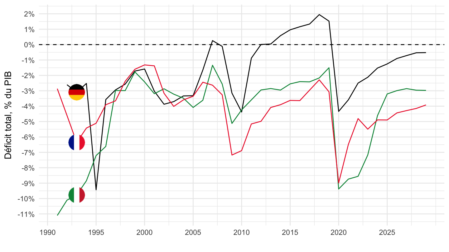
2013, Facet
Code
GGCB_G01_PGDP_PT %>%
  bind_rows(GGCBP_G01_PGDP_PT) %>%
  bind_rows(GGXCNL_G01_GDP_PT) %>%
  bind_rows(GGXONLB_G01_GDP_PT) %>%
  filter(REF_AREA %in% c("FR", "IT", "DE")) %>%
  left_join(REF_AREA, by = "REF_AREA") %>%
  year_to_date2() %>%
  mutate(primary = ifelse(INDICATOR %in% c("GGCBP_G01_PGDP_PT", "GGXONLB_G01_GDP_PT"), "Primary Deficit", "Total Deficit"),
         cyclically = ifelse(INDICATOR %in% c("GGCBP_G01_PGDP_PT", "GGCB_G01_PGDP_PT"), "Cyclically Adjusted Public deficit\n% of potential GDP", "Public Deficit\n% of GDP"),
         primary = factor(primary, levels = c("Total Deficit", "Primary Deficit")),
         cyclically = factor(cyclically, levels = c("Public Deficit\n% of GDP", "Cyclically Adjusted Public deficit\n% of potential GDP"))) %>%
  mutate(OBS_VALUE = OBS_VALUE/100) %>%
  filter(date >= as.Date("2013-01-01")) %>%
  ggplot(.) + geom_line(aes(x = date, y = OBS_VALUE, color = Ref_area, linetype = primary)) +
  theme_minimal() + xlab("") + ylab("Public deficit (%)") +
  scale_x_date(breaks = seq(1921, 2100, 2) %>% paste0("-01-01") %>% as.Date,
               labels = date_format("%Y")) +
  theme(legend.position = "top",
        legend.title = element_blank(),
        axis.text.x = element_text(angle = 45, vjust = 1, hjust = 1)) +
  scale_y_continuous(breaks = 0.01*seq(-60, 60, 1),
                     labels = scales::percent_format(accuracy = 1)) +
  scale_color_manual(values = c("#ED2939", "#000000", "#009246")) +
  facet_wrap(~ cyclically)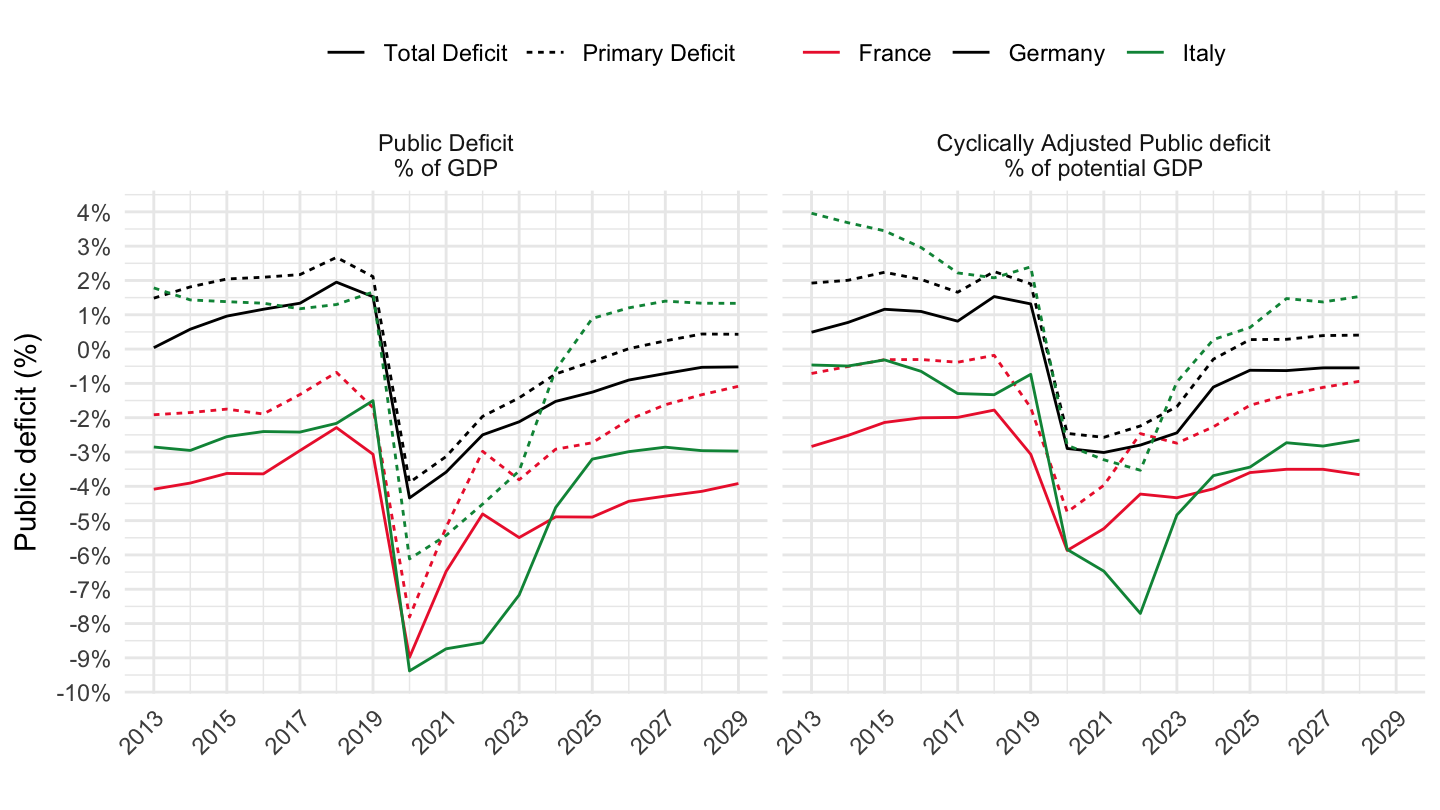
Australia, United Kingdom, United States
Code
GGXCNL_G01_GDP_PT %>%
  filter(REF_AREA %in% c("GB", "US", "AU")) %>%
  left_join(REF_AREA, by = "REF_AREA") %>%
  year_to_date2() %>%
  left_join(colors, by = c("Ref_area" = "country")) %>%
  mutate(color = ifelse(REF_AREA == "US", color2, color)) %>%
  mutate(OBS_VALUE = OBS_VALUE/100) %>%
  rename(Counterpart_area = Ref_area) %>%
  #filter(date <= as.Date("2021-01-01")) %>%
  ggplot(.) + geom_line(aes(x = date, y = OBS_VALUE, color = color)) +
  theme_minimal() + xlab("") + ylab("Déficit total, % du PIB") +
  scale_color_identity() + add_3flags +
  scale_x_date(breaks = seq(1920, 2100, 5) %>% paste0("-01-01") %>% as.Date,
               labels = date_format("%Y")) +
  scale_y_continuous(breaks = 0.01*seq(-60, 60, 1),
                     labels = scales::percent_format(accuracy = 1)) +
  geom_hline(yintercept = 0, linetype = "dashed", color = "black")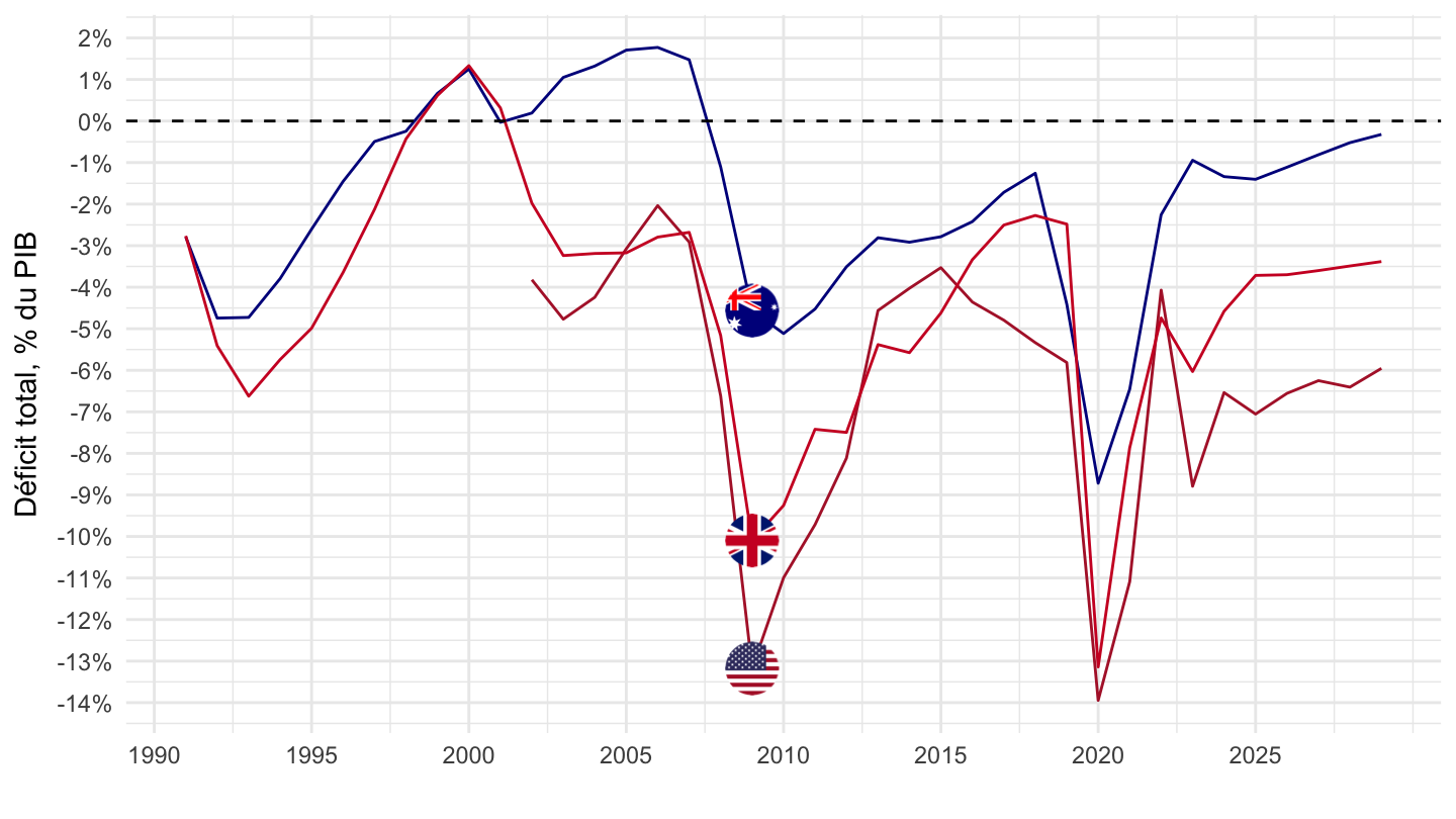
Euro area vs US
2002-
Code
GGCB_G01_PGDP_PT %>%
  bind_rows(GGCBP_G01_PGDP_PT) %>%
  bind_rows(GGXCNL_G01_GDP_PT) %>%
  bind_rows(GGXONLB_G01_GDP_PT) %>%
  filter(REF_AREA %in% c("U2", "US")) %>%
  year_to_date2() %>%
  mutate(Ref_area = ifelse(REF_AREA == "U2", "Euro area", "US"),
         primary = ifelse(INDICATOR %in% c("GGCBP_G01_PGDP_PT", "GGXONLB_G01_GDP_PT"), "Primary Deficit", "Total Deficit"),
         cyclically = ifelse(INDICATOR %in% c("GGCBP_G01_PGDP_PT", "GGCB_G01_PGDP_PT"), "Cyclically Adjusted (% of potential GDP)", "Actual Deficit (% of GDP)")) %>%
  mutate(OBS_VALUE = OBS_VALUE/100) %>%
  filter(date >= as.Date("2002-01-01")) %>%
  ggplot(.) + geom_line(aes(x = date, y = OBS_VALUE, color = Ref_area, linetype = primary)) +
  theme_minimal() + xlab("") + ylab("Public deficit, % of GDP") +
  scale_x_date(breaks = seq(1920, 2100, 5) %>% paste0("-01-01") %>% as.Date,
               labels = date_format("%Y")) +
  theme(legend.position = c(0.3, 0.78),
        legend.title = element_blank(),
        axis.text.x = element_text(angle = 45, vjust = 1, hjust = 1)) +
  scale_y_continuous(breaks = 0.01*seq(-60, 60, 1),
                     labels = scales::percent_format(accuracy = 1)) +
  scale_color_manual(values = c("#003399", "#B22234")) +
  facet_wrap(~ cyclically)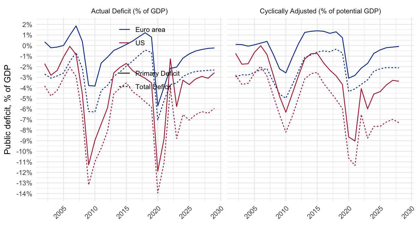
2005-
Code
GGCB_G01_PGDP_PT %>%
  bind_rows(GGCBP_G01_PGDP_PT) %>%
  bind_rows(GGXCNL_G01_GDP_PT) %>%
  bind_rows(GGXONLB_G01_GDP_PT) %>%
  filter(REF_AREA %in% c("U2", "US")) %>%
  year_to_date2() %>%
  mutate(Ref_area = ifelse(REF_AREA == "U2", "Euro area", "US"),
         primary = ifelse(INDICATOR %in% c("GGCBP_G01_PGDP_PT", "GGXONLB_G01_GDP_PT"), "Primary Deficit", "Total Deficit"),
         cyclically = ifelse(INDICATOR %in% c("GGCBP_G01_PGDP_PT", "GGCB_G01_PGDP_PT"), "Cyclically Adjusted Public deficit\n% of potential GDP", "Public Deficit\n% of GDP"),
         primary = factor(primary, levels = c("Total Deficit", "Primary Deficit")),
         cyclically = factor(cyclically, levels = c("Public Deficit\n% of GDP", "Cyclically Adjusted Public deficit\n% of potential GDP"))) %>%
  mutate(OBS_VALUE = OBS_VALUE/100) %>%
  filter(date >= as.Date("2005-01-01")) %>%
  ggplot(.) + geom_line(aes(x = date, y = OBS_VALUE, color = Ref_area, linetype = primary)) +
  theme_minimal() + xlab("") + ylab("Public deficit (%)") +
  scale_x_date(breaks = seq(1921, 2100, 2) %>% paste0("-01-01") %>% as.Date,
               labels = date_format("%Y")) +
  theme(legend.position = "top",
        legend.title = element_blank(),
        axis.text.x = element_text(angle = 45, vjust = 1, hjust = 1)) +
  scale_y_continuous(breaks = 0.01*seq(-60, 60, 1),
                     labels = scales::percent_format(accuracy = 1)) +
  scale_color_manual(values = c("#003399", "#B22234")) +
  facet_wrap(~ cyclically)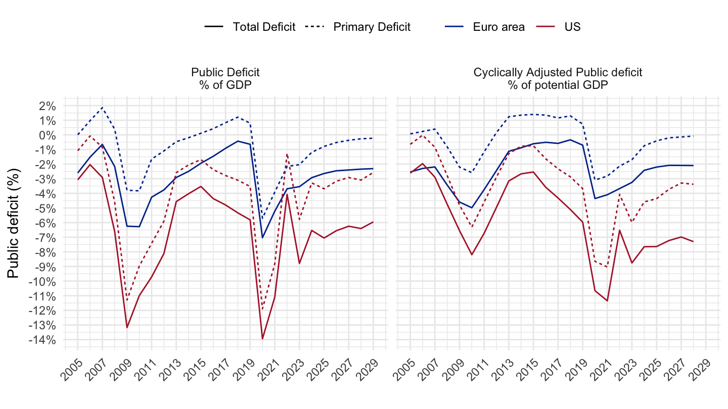
2010-
English
Code
GGCB_G01_PGDP_PT %>%
  bind_rows(GGCBP_G01_PGDP_PT) %>%
  bind_rows(GGXCNL_G01_GDP_PT) %>%
  bind_rows(GGXONLB_G01_GDP_PT) %>%
  filter(REF_AREA %in% c("U2", "US")) %>%
  year_to_date2() %>%
  mutate(Ref_area = ifelse(REF_AREA == "U2", "Euro area", "US"),
         primary = ifelse(INDICATOR %in% c("GGCBP_G01_PGDP_PT", "GGXONLB_G01_GDP_PT"), "Primary Deficit", "Total Deficit"),
         cyclically = ifelse(INDICATOR %in% c("GGCBP_G01_PGDP_PT", "GGCB_G01_PGDP_PT"), "Cyclically Adjusted Public deficit\n% of potential GDP", "Public Deficit\n% of GDP"),
         primary = factor(primary, levels = c("Total Deficit", "Primary Deficit")),
         cyclically = factor(cyclically, levels = c("Public Deficit\n% of GDP", "Cyclically Adjusted Public deficit\n% of potential GDP"))) %>%
  mutate(OBS_VALUE = OBS_VALUE/100) %>%
  filter(date >= as.Date("2010-01-01")) %>%
  ggplot(.) + geom_line(aes(x = date, y = OBS_VALUE, color = Ref_area, linetype = primary)) +
  theme_minimal() + xlab("") + ylab("Public deficit (%)") +
  scale_x_date(breaks = seq(1921, 2100, 2) %>% paste0("-01-01") %>% as.Date,
               labels = date_format("%Y")) +
  theme(legend.position = "top",
        legend.title = element_blank(),
        axis.text.x = element_text(angle = 45, vjust = 1, hjust = 1)) +
  scale_y_continuous(breaks = 0.01*seq(-60, 60, 1),
                     labels = scales::percent_format(accuracy = 1)) +
  scale_color_manual(values = c("#003399", "#B22234")) +
  facet_wrap(~ cyclically)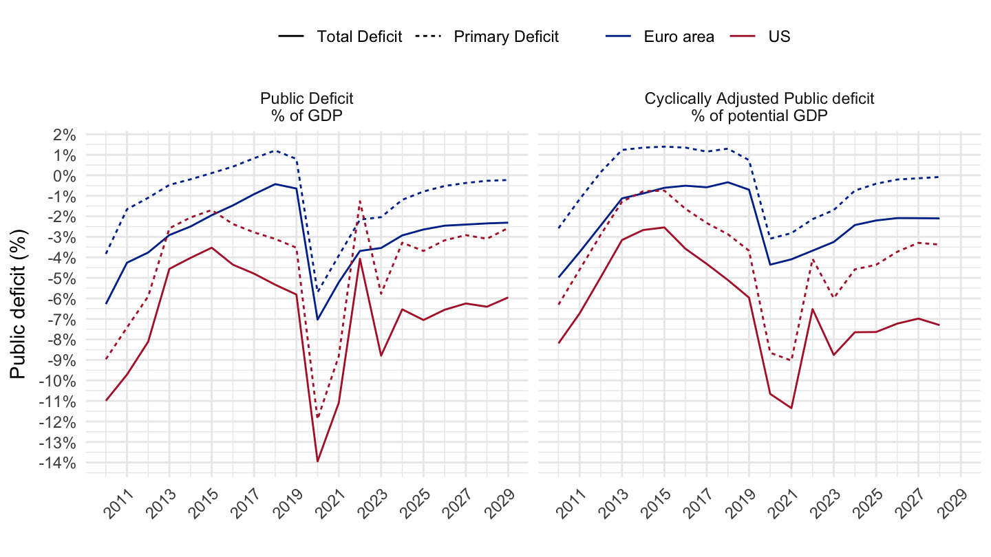
French
Code
GGCB_G01_PGDP_PT %>%
  bind_rows(GGCBP_G01_PGDP_PT) %>%
  bind_rows(GGXCNL_G01_GDP_PT) %>%
  bind_rows(GGXONLB_G01_GDP_PT) %>%
  filter(REF_AREA %in% c("U2", "US")) %>%
  year_to_date2() %>%
  mutate(Ref_area = ifelse(REF_AREA == "U2", "Zone euro", "États-Unis"),
         Ref_area = factor(Ref_area, levels = c("Zone euro", "États-Unis")),
         Counterpart_area = ifelse(REF_AREA == "U2", "Europe", "United States"),
         primary = ifelse(INDICATOR %in% c("GGCBP_G01_PGDP_PT", "GGXONLB_G01_GDP_PT"), "Déficit primaire", "Déficit total"),
         cyclically = ifelse(INDICATOR %in% c("GGCBP_G01_PGDP_PT", "GGCB_G01_PGDP_PT"), "Déficit public ajusté du cycle\n% du PIB potentiel", "Déficit public\n% du PIB"),
         primary = factor(primary, levels = c("Déficit total", "Déficit primaire")),
         cyclically = factor(cyclically, levels = c("Déficit public\n% du PIB", "Déficit public ajusté du cycle\n% du PIB potentiel"))) %>%
  mutate(OBS_VALUE = OBS_VALUE/100) %>%
  filter(date >= as.Date("2010-01-01")) %>%
  ggplot(.) + geom_line(aes(x = date, y = OBS_VALUE, color = Ref_area, linetype = primary)) +
  theme_minimal() + xlab("") + ylab("Déficit public (%)") +
  scale_x_date(breaks = seq(1920, 2100, 1) %>% paste0("-01-01") %>% as.Date,
               labels = date_format("%Y")) +
  scale_linetype_manual(values = c("solid", "dashed")) +
  add_8flags +
  theme(legend.position = "top",
        legend.title = element_blank(),
        axis.text.x = element_text(angle = 45, vjust = 1, hjust = 1)) +
  scale_y_continuous(breaks = 0.01*seq(-60, 60, 1),
                     labels = scales::percent_format(accuracy = 1)) +
  scale_color_manual(values = c("#003399", "#B22234")) +
  facet_wrap(~ cyclically)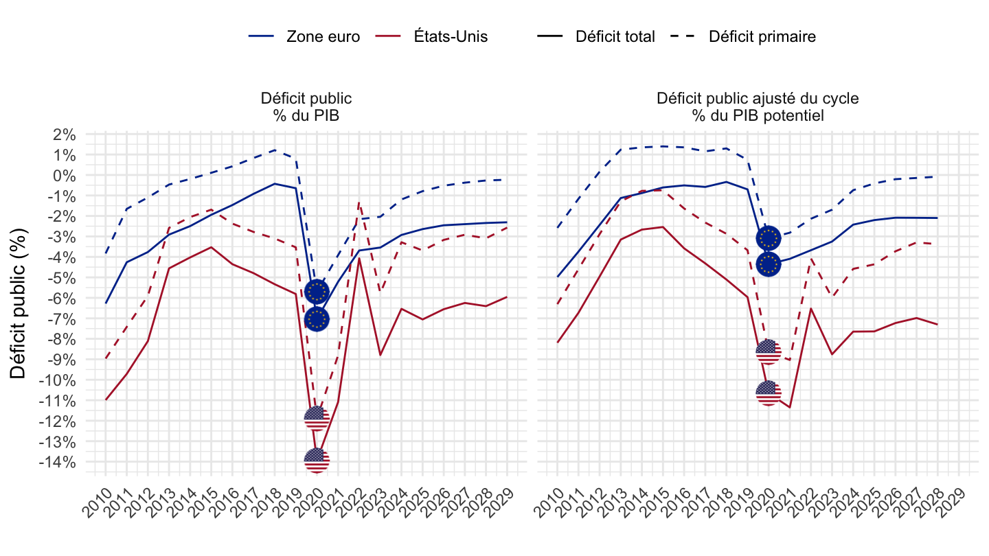
2013-
English
Code
GGCB_G01_PGDP_PT %>%
  bind_rows(GGCBP_G01_PGDP_PT) %>%
  bind_rows(GGXCNL_G01_GDP_PT) %>%
  bind_rows(GGXONLB_G01_GDP_PT) %>%
  filter(REF_AREA %in% c("U2", "US")) %>%
  year_to_date2() %>%
  mutate(Ref_area = ifelse(REF_AREA == "U2", "Euro area", "US"),
         primary = ifelse(INDICATOR %in% c("GGCBP_G01_PGDP_PT", "GGXONLB_G01_GDP_PT"), "Primary Deficit", "Total Deficit"),
         cyclically = ifelse(INDICATOR %in% c("GGCBP_G01_PGDP_PT", "GGCB_G01_PGDP_PT"), "Cyclically Adjusted Public deficit\n% of potential GDP", "Public Deficit\n% of GDP"),
         primary = factor(primary, levels = c("Total Deficit", "Primary Deficit")),
         cyclically = factor(cyclically, levels = c("Public Deficit\n% of GDP", "Cyclically Adjusted Public deficit\n% of potential GDP"))) %>%
  mutate(OBS_VALUE = OBS_VALUE/100) %>%
  filter(date >= as.Date("2013-01-01")) %>%
  ggplot(.) + geom_line(aes(x = date, y = OBS_VALUE, color = Ref_area, linetype = primary)) +
  theme_minimal() + xlab("") + ylab("Public deficit (%)") +
  scale_x_date(breaks = seq(1921, 2100, 2) %>% paste0("-01-01") %>% as.Date,
               labels = date_format("%Y")) +
  theme(legend.position = "top",
        legend.title = element_blank(),
        axis.text.x = element_text(angle = 45, vjust = 1, hjust = 1)) +
  scale_y_continuous(breaks = 0.01*seq(-60, 60, 1),
                     labels = scales::percent_format(accuracy = 1)) +
  scale_color_manual(values = c("#003399", "#B22234")) +
  facet_wrap(~ cyclically)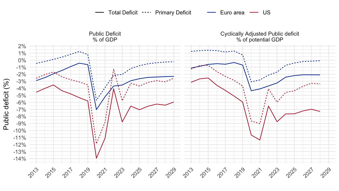
French
Code
GGCB_G01_PGDP_PT %>%
  bind_rows(GGCBP_G01_PGDP_PT) %>%
  bind_rows(GGXCNL_G01_GDP_PT) %>%
  bind_rows(GGXONLB_G01_GDP_PT) %>%
  filter(REF_AREA %in% c("U2", "US")) %>%
  year_to_date2() %>%
  mutate(Ref_area = ifelse(REF_AREA == "U2", "Zone euro", "États-Unis"),
         Ref_area = factor(Ref_area, levels = c("Zone euro", "États-Unis")),
         Counterpart_area = ifelse(REF_AREA == "U2", "Europe", "United States"),
         primary = ifelse(INDICATOR %in% c("GGCBP_G01_PGDP_PT", "GGXONLB_G01_GDP_PT"), "Déficit primaire", "Déficit total"),
         cyclically = ifelse(INDICATOR %in% c("GGCBP_G01_PGDP_PT", "GGCB_G01_PGDP_PT"), "Déficit public ajusté du cycle\n% du PIB potentiel", "Déficit public\n% du PIB"),
         primary = factor(primary, levels = c("Déficit total", "Déficit primaire")),
         cyclically = factor(cyclically, levels = c("Déficit public\n% du PIB", "Déficit public ajusté du cycle\n% du PIB potentiel"))) %>%
  mutate(OBS_VALUE = OBS_VALUE/100) %>%
  filter(date >= as.Date("2013-01-01")) %>%
  ggplot(.) + geom_line(aes(x = date, y = OBS_VALUE, color = Ref_area, linetype = primary)) +
  theme_minimal() + xlab("") + ylab("Déficit public (%)") +
  scale_x_date(breaks = seq(1920, 2100, 1) %>% paste0("-01-01") %>% as.Date,
               labels = date_format("%Y")) +
  scale_linetype_manual(values = c("solid", "dashed")) +
  add_8flags +
  theme(legend.position = "top",
        legend.title = element_blank(),
        axis.text.x = element_text(angle = 45, vjust = 1, hjust = 1)) +
  scale_y_continuous(breaks = 0.01*seq(-60, 60, 1),
                     labels = scales::percent_format(accuracy = 1)) +
  scale_color_manual(values = c("#003399", "#B22234")) +
  facet_wrap(~ cyclically)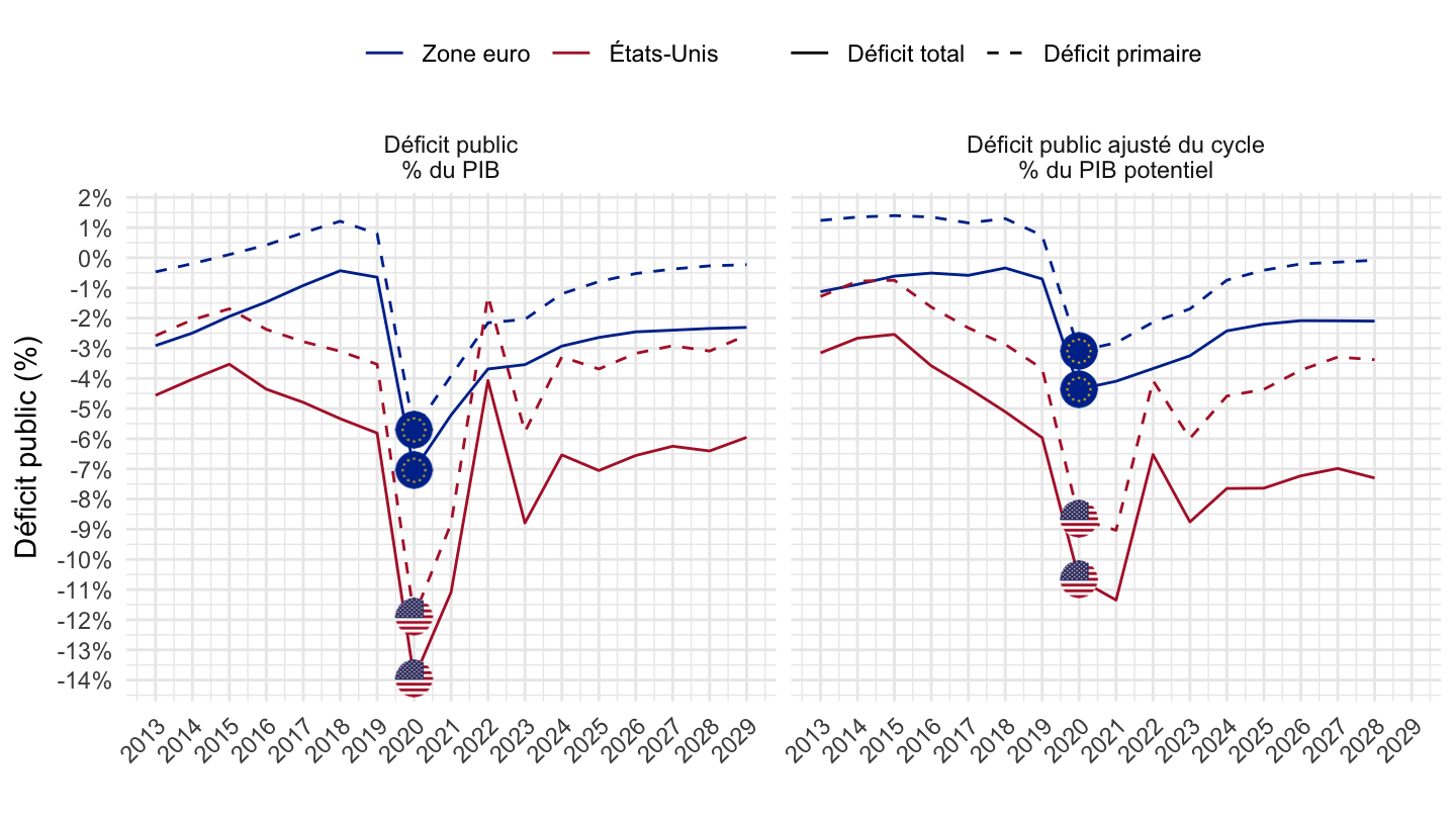
Euro area, United States, Germany
All
Code
GGXCNL_G01_GDP_PT %>%
  filter(REF_AREA %in% c("U2", "US")) %>%
  left_join(REF_AREA, by = "REF_AREA") %>%
  year_to_date2() %>%
  mutate(Ref_area = ifelse(REF_AREA == "U2", "Europe", Ref_area)) %>%
  left_join(colors, by = c("Ref_area" = "country")) %>%
  mutate(color = ifelse(REF_AREA == "US", color2, color)) %>%
  mutate(OBS_VALUE = OBS_VALUE/100) %>%
  rename(Counterpart_area = Ref_area) %>%
  filter(date >= as.Date("1999-01-01")) %>%
  ggplot(.) + geom_line(aes(x = date, y = OBS_VALUE, color = color)) +
  theme_minimal() + xlab("") + ylab("Déficit total, % du PIB") +
  scale_color_identity() + add_2flags +
  scale_x_date(breaks = c(seq(1999, 2100, 5), seq(1997, 2100, 5)) %>% paste0("-01-01") %>% as.Date,
               labels = date_format("%Y")) +
  scale_y_continuous(breaks = 0.01*seq(-60, 60, 1),
                     labels = scales::percent_format(accuracy = 1)) +
  geom_hline(yintercept = 0, linetype = "dashed", color = "black") +
  geom_hline(yintercept = -0.03, linetype = "dashed", color = "black")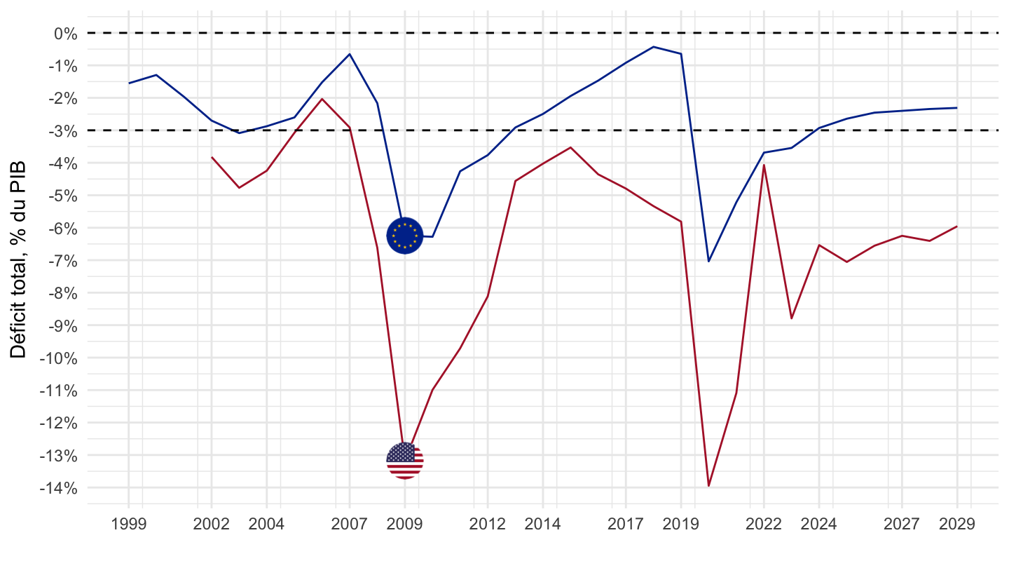
2003-
Code
GGXCNL_G01_GDP_PT %>%
  filter(REF_AREA %in% c("U2", "US")) %>%
  left_join(REF_AREA, by = "REF_AREA") %>%
  year_to_date2() %>%
  mutate(Ref_area = ifelse(REF_AREA == "U2", "Europe", Ref_area)) %>%
  left_join(colors, by = c("Ref_area" = "country")) %>%
  mutate(color = ifelse(REF_AREA == "US", color2, color)) %>%
  mutate(OBS_VALUE = OBS_VALUE/100) %>%
  rename(Counterpart_area = Ref_area) %>%
  filter(date >= as.Date("2003-01-01")) %>%
  ggplot(.) + geom_line(aes(x = date, y = OBS_VALUE, color = color)) +
  theme_minimal() + xlab("") + ylab("Déficit total, % du PIB") +
  scale_color_identity() + add_2flags +
  scale_x_date(breaks = c(seq(2003, 2100, 2)) %>% paste0("-01-01") %>% as.Date,
               labels = date_format("%Y")) +
  scale_y_continuous(breaks = 0.01*seq(-60, 60, 1),
                     labels = scales::percent_format(accuracy = 1)) +
  geom_hline(yintercept = 0, linetype = "dashed", color = "black") +
  geom_hline(yintercept = -0.03, linetype = "dashed", color = "black")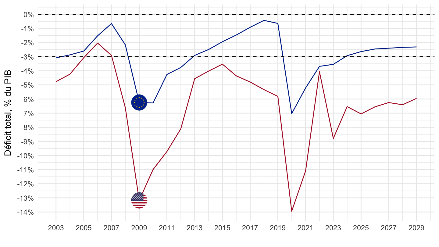
1999-2023
Code
plot <- GGXCNL_G01_GDP_PT %>%
  filter(REF_AREA %in% c("U2", "US")) %>%
  left_join(REF_AREA, by = "REF_AREA") %>%
  year_to_date2() %>%
  mutate(Ref_area = ifelse(REF_AREA == "U2", "Zone euro", "États-Unis")) %>%
  filter(date >= as.Date("1999-01-01"),
         date <= as.Date("2023-01-01")) %>%
  ggplot(.) + geom_line(aes(x = date, y = OBS_VALUE/100, color = Ref_area)) +
  scale_color_manual(values = c("#B22234", "#003399")) +
  theme_minimal() + xlab("") + ylab("Solde des Administrations Publiques, % du PIB") +
  scale_x_date(breaks = c(seq(1999, 2100, 5), seq(1997, 2100, 5)) %>% paste0("-01-01") %>% as.Date,
               labels = date_format("%Y")) +
  scale_y_continuous(breaks = 0.01*seq(-60, 60, 1),
                     labels = scales::percent_format(accuracy = 1)) +
  geom_hline(yintercept = 0, linetype = "dashed", color = "black") +
  geom_hline(yintercept = -0.03, linetype = "dashed", color = "black") +
  geom_rect(data = nber_recessions %>%
              filter(Peak > as.Date("1999-01-01")),
            aes(xmin = Peak, xmax = Trough, ymin = -Inf, ymax = +Inf),
            fill = '#B22234', alpha = 0.1)  +
  geom_rect(data = cepr_recessions %>%
              filter(Peak > as.Date("1999-01-01")),
            aes(xmin = Peak, xmax = Trough, ymin = -Inf, ymax = +Inf),
            fill = '#003399', alpha = 0.1) +
  theme(legend.position = c(0.2, 0.2),
        legend.title = element_blank()) +
  labs(caption = "Source: Fonds Monétaire International, Fiscal Monitor")

plot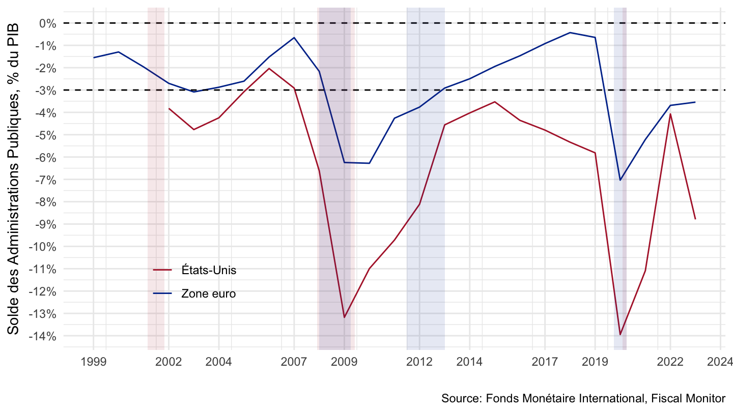
Code
save(plot, file = "GGXCNL_G01_GDP_PT_files/figure-html/U2-US-1999-2023-1.RData")France, United States
1995-
Code
GGXCNL_G01_GDP_PT %>%
  filter(REF_AREA %in% c("FR", "US")) %>%
  left_join(REF_AREA, by = "REF_AREA") %>%
  year_to_date2() %>%
  left_join(colors, by = c("Ref_area" = "country")) %>%
  mutate(OBS_VALUE = OBS_VALUE/100) %>%
  rename(Counterpart_area = Ref_area) %>%
  filter(date >= as.Date("1995-01-01")) %>%
  ggplot(.) + geom_line(aes(x = date, y = OBS_VALUE, color = color)) +
  theme_minimal() + xlab("") + ylab("Déficit total, % du PIB") +
  scale_color_identity() + add_2flags +
  scale_x_date(breaks = seq(1920, 2100, 5) %>% paste0("-01-01") %>% as.Date,
               labels = date_format("%Y")) +
  scale_y_continuous(breaks = 0.01*seq(-60, 60, 1),
                     labels = scales::percent_format(accuracy = 1)) +
  geom_hline(yintercept = 0, linetype = "dashed", color = "black")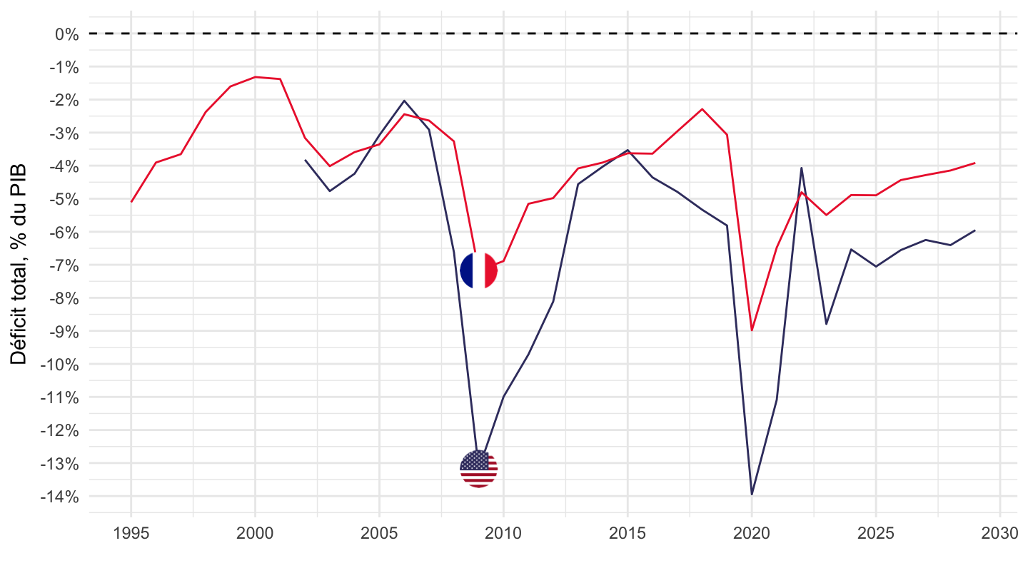
2002-2023
Code
GGXCNL_G01_GDP_PT %>%
  filter(REF_AREA %in% c("FR", "US")) %>%
  left_join(REF_AREA, by = "REF_AREA") %>%
  year_to_date2() %>%
  left_join(colors, by = c("Ref_area" = "country")) %>%
  mutate(OBS_VALUE = OBS_VALUE/100) %>%
  rename(Counterpart_area = Ref_area) %>%
  filter(date >= as.Date("2002-01-01"),
         date <= as.Date("2023-01-01")) %>%
  ggplot(.) + geom_line(aes(x = date, y = OBS_VALUE, color = color)) +
  theme_minimal() + xlab("") + ylab("Déficit total, % du PIB") +
  scale_color_identity() + add_2flags +
  scale_x_date(breaks = seq(1920, 2100, 2) %>% paste0("-01-01") %>% as.Date,
               labels = date_format("%Y")) +
  scale_y_continuous(breaks = 0.01*seq(-60, 60, 1),
                     labels = scales::percent_format(accuracy = 1)) +
  geom_hline(yintercept = 0, linetype = "dashed", color = "black")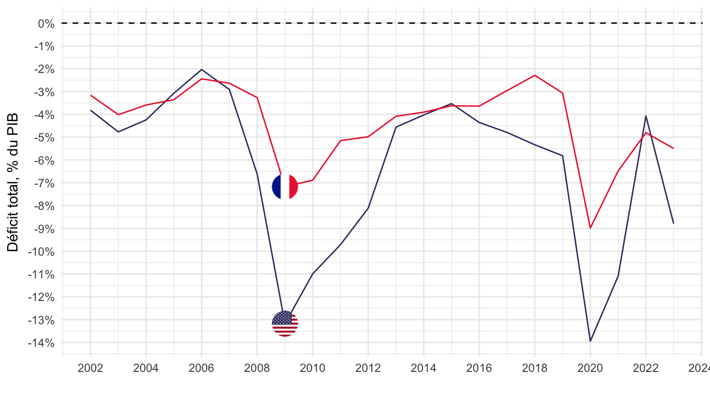
2002-
Code
GGXCNL_G01_GDP_PT %>%
  filter(REF_AREA %in% c("FR", "US")) %>%
  left_join(REF_AREA, by = "REF_AREA") %>%
  year_to_date2() %>%
  left_join(colors, by = c("Ref_area" = "country")) %>%
  mutate(OBS_VALUE = OBS_VALUE/100) %>%
  rename(Counterpart_area = Ref_area) %>%
  filter(date >= as.Date("2002-01-01")) %>%
  ggplot(.) + geom_line(aes(x = date, y = OBS_VALUE, color = color)) +
  theme_minimal() + xlab("") + ylab("Déficit total, % du PIB") +
  scale_color_identity() + add_2flags +
  scale_x_date(breaks = seq(1920, 2100, 2) %>% paste0("-01-01") %>% as.Date,
               labels = date_format("%Y")) +
  scale_y_continuous(breaks = 0.01*seq(-60, 60, 1),
                     labels = scales::percent_format(accuracy = 1)) +
  geom_hline(yintercept = 0, linetype = "dashed", color = "black")
Euro area, United States, Germany
All
Code
GGXCNL_G01_GDP_PT %>%
  filter(REF_AREA %in% c("U2", "US", "DE")) %>%
  left_join(REF_AREA, by = "REF_AREA") %>%
  year_to_date2() %>%
  mutate(Ref_area = ifelse(REF_AREA == "U2", "Europe", Ref_area)) %>%
  left_join(colors, by = c("Ref_area" = "country")) %>%
  mutate(color = ifelse(REF_AREA == "US", color2, color)) %>%
  mutate(OBS_VALUE = OBS_VALUE/100) %>%
  rename(Counterpart_area = Ref_area) %>%
  #filter(date <= as.Date("2021-01-01")) %>%
  ggplot(.) + geom_line(aes(x = date, y = OBS_VALUE, color = color)) +
  theme_minimal() + xlab("") + ylab("Déficit total, % du PIB") +
  scale_color_identity() + add_3flags +
  scale_x_date(breaks = seq(1920, 2100, 5) %>% paste0("-01-01") %>% as.Date,
               labels = date_format("%Y")) +
  scale_y_continuous(breaks = 0.01*seq(-60, 60, 1),
                     labels = scales::percent_format(accuracy = 1)) +
  geom_hline(yintercept = 0, linetype = "dashed", color = "black")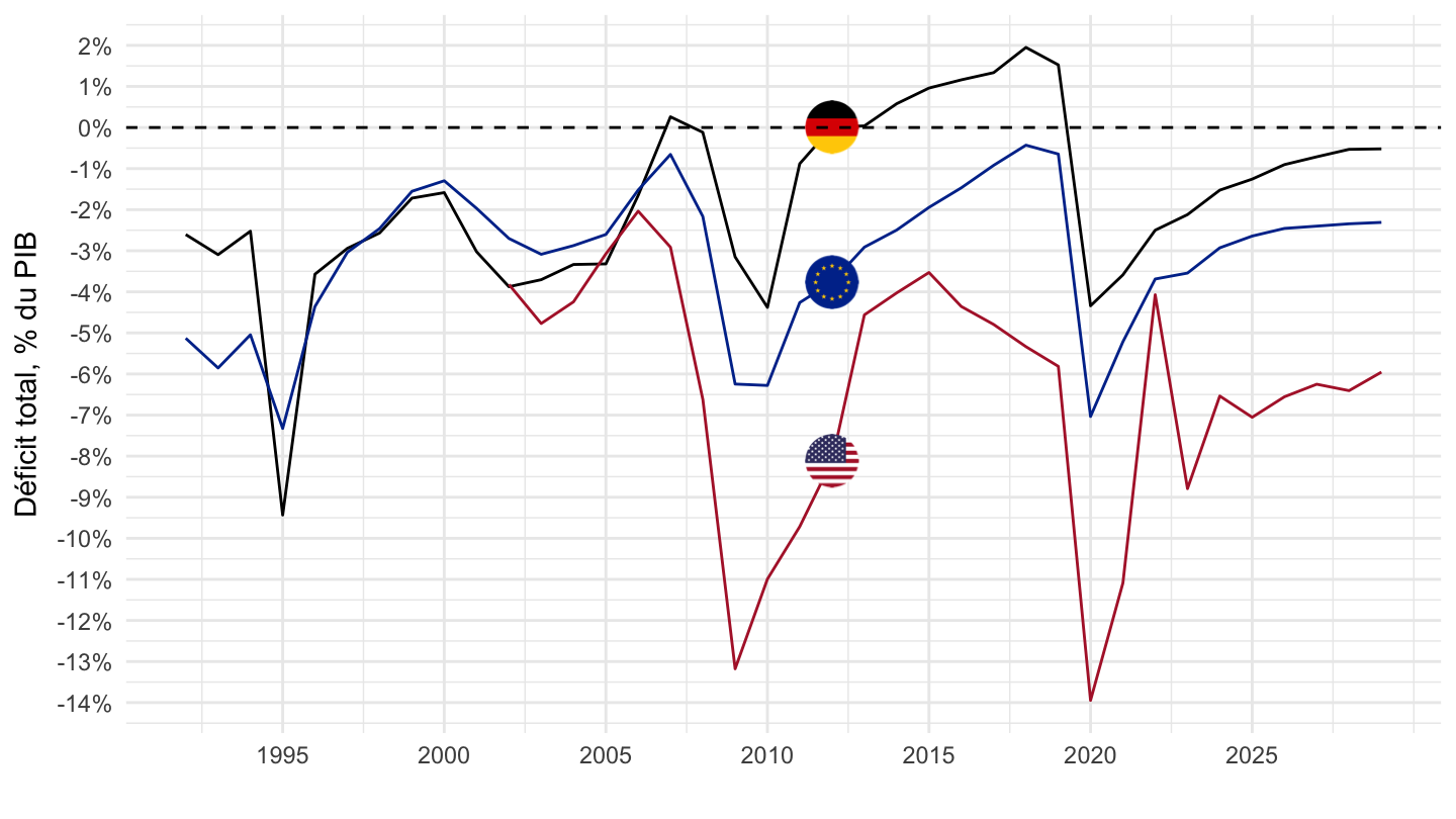
Euro area, United States, France
All
Code
GGXCNL_G01_GDP_PT %>%
  filter(REF_AREA %in% c("U2", "US", "FR")) %>%
  left_join(REF_AREA, by = "REF_AREA") %>%
  year_to_date2() %>%
  mutate(Ref_area = ifelse(REF_AREA == "U2", "Europe", Ref_area)) %>%
  left_join(colors, by = c("Ref_area" = "country")) %>%
  mutate(color = ifelse(REF_AREA == "US", color2, color)) %>%
  mutate(OBS_VALUE = OBS_VALUE/100) %>%
  rename(Counterpart_area = Ref_area) %>%
  #filter(date <= as.Date("2021-01-01")) %>%
  ggplot(.) + geom_line(aes(x = date, y = OBS_VALUE, color = color)) +
  theme_minimal() + xlab("") + ylab("Déficit total, % du PIB") +
  scale_color_identity() + add_3flags +
  scale_x_date(breaks = seq(1920, 2100, 5) %>% paste0("-01-01") %>% as.Date,
               labels = date_format("%Y")) +
  scale_y_continuous(breaks = 0.01*seq(-60, 60, 1),
                     labels = scales::percent_format(accuracy = 1)) +
  geom_hline(yintercept = 0, linetype = "dashed", color = "black")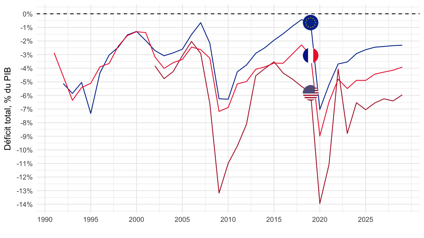
2010-
Code
GGXCNL_G01_GDP_PT %>%
  filter(REF_AREA %in% c("U2", "US", "FR")) %>%
  left_join(REF_AREA, by = "REF_AREA") %>%
  year_to_date2() %>%
  mutate(Ref_area = ifelse(REF_AREA == "U2", "Europe", Ref_area)) %>%
  left_join(colors, by = c("Ref_area" = "country")) %>%
  mutate(color = ifelse(REF_AREA == "U2", color2, color)) %>%
  mutate(OBS_VALUE = OBS_VALUE/100) %>%
  rename(Counterpart_area = Ref_area) %>%
  filter(date >= as.Date("2010-01-01")) %>%
  ggplot(.) + geom_line(aes(x = date, y = OBS_VALUE, color = color)) +
  theme_minimal() + xlab("") + ylab("Déficit total, % du PIB") +
  scale_color_identity() + add_3flags +
  scale_x_date(breaks = seq(1920, 2100, 1) %>% paste0("-01-01") %>% as.Date,
               labels = date_format("%Y")) +
  scale_y_continuous(breaks = 0.01*seq(-60, 60, 1),
                     labels = scales::percent_format(accuracy = 1)) +
  geom_hline(yintercept = 0, linetype = "dashed", color = "black")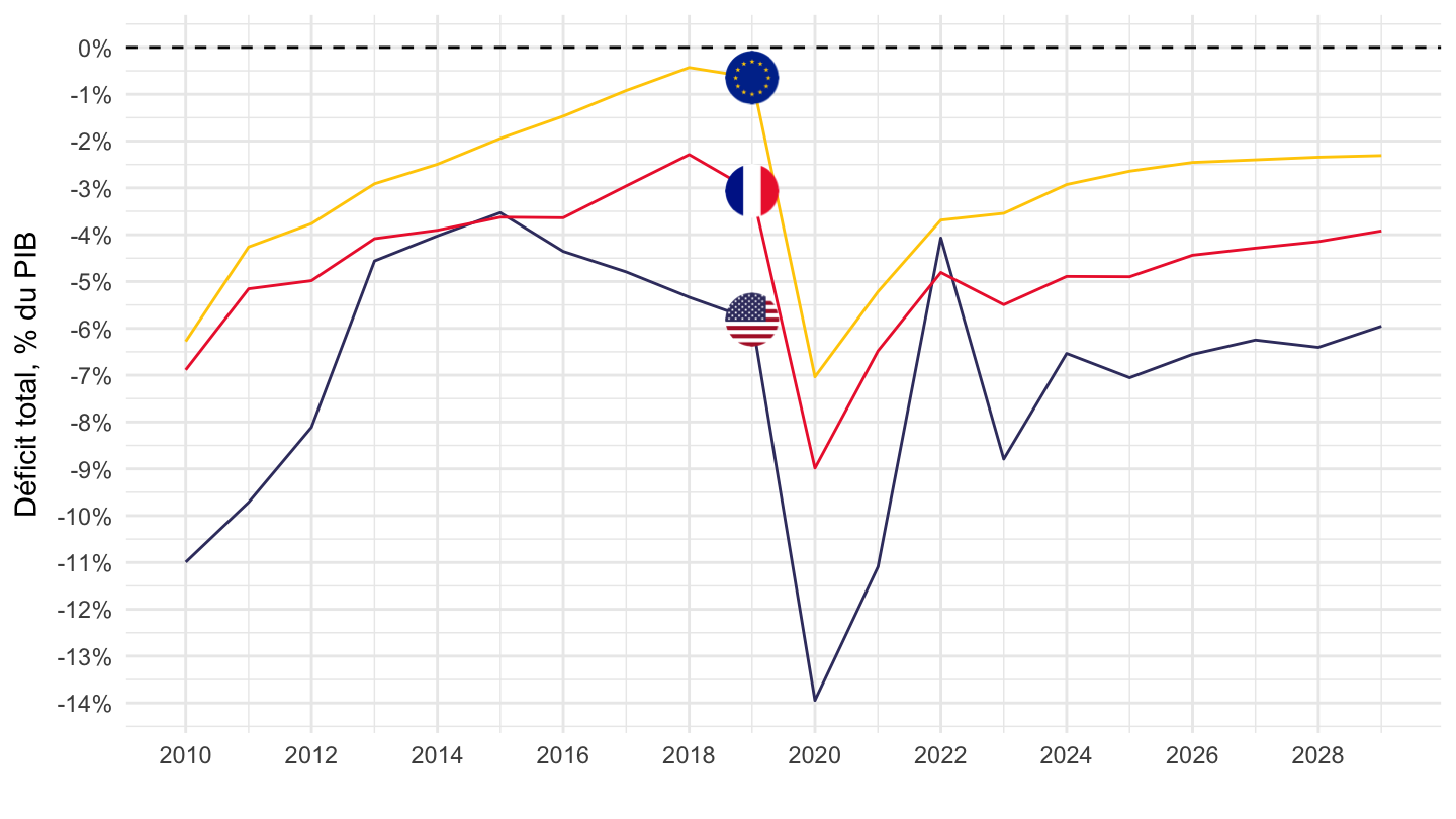
Euro area, United States, France, Germany
All
Code
GGXCNL_G01_GDP_PT %>%
  filter(REF_AREA %in% c("U2", "US", "FR", "DE")) %>%
  left_join(REF_AREA, by = "REF_AREA") %>%
  year_to_date2() %>%
  mutate(Ref_area = ifelse(REF_AREA == "U2", "Europe", Ref_area)) %>%
  left_join(colors, by = c("Ref_area" = "country")) %>%
  mutate(color = ifelse(REF_AREA == "US", color2, color)) %>%
  mutate(OBS_VALUE = OBS_VALUE/100) %>%
  rename(Counterpart_area = Ref_area) %>%
  #filter(date <= as.Date("2021-01-01")) %>%
  ggplot(.) + geom_line(aes(x = date, y = OBS_VALUE, color = color)) +
  theme_minimal() + xlab("") + ylab("Déficit total, % du PIB") +
  scale_color_identity() + add_3flags +
  scale_x_date(breaks = seq(1920, 2100, 5) %>% paste0("-01-01") %>% as.Date,
               labels = date_format("%Y")) +
  scale_y_continuous(breaks = 0.01*seq(-60, 60, 1),
                     labels = scales::percent_format(accuracy = 1)) +
  geom_hline(yintercept = 0, linetype = "dashed", color = "black")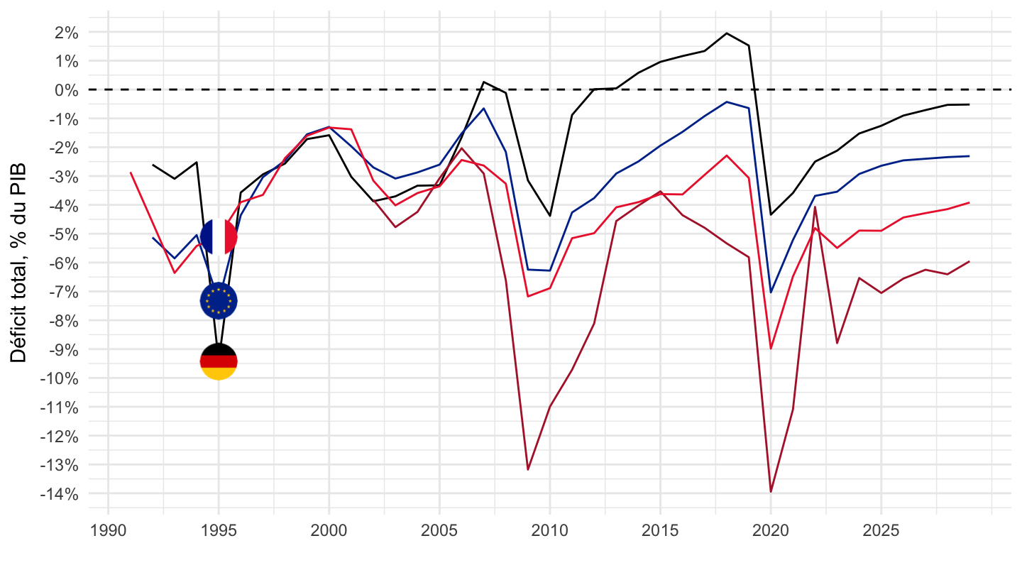
2010-
Code
GGXCNL_G01_GDP_PT %>%
  filter(REF_AREA %in% c("U2", "US", "FR", "DE")) %>%
  left_join(REF_AREA, by = "REF_AREA") %>%
  year_to_date2() %>%
  mutate(Ref_area = ifelse(REF_AREA == "U2", "Europe", Ref_area)) %>%
  left_join(colors, by = c("Ref_area" = "country")) %>%
  mutate(color = ifelse(REF_AREA == "U2", color2, color)) %>%
  mutate(OBS_VALUE = OBS_VALUE/100) %>%
  rename(Counterpart_area = Ref_area) %>%
  filter(date >= as.Date("2010-01-01")) %>%
  ggplot(.) + geom_line(aes(x = date, y = OBS_VALUE, color = color)) +
  theme_minimal() + xlab("") + ylab("Déficit total, % du PIB") +
  scale_color_identity() + add_4flags +
  scale_x_date(breaks = seq(1920, 2100, 1) %>% paste0("-01-01") %>% as.Date,
               labels = date_format("%Y")) +
  scale_y_continuous(breaks = 0.01*seq(-60, 60, 1),
                     labels = scales::percent_format(accuracy = 1)) +
  geom_hline(yintercept = 0, linetype = "dashed", color = "black") +
  theme(axis.text.x = element_text(angle = 45, vjust = 1, hjust = 1)) +
  geom_label(data = . %>% filter(date == max(date)), aes(x = date, y = OBS_VALUE, color = color, label = percent(OBS_VALUE)))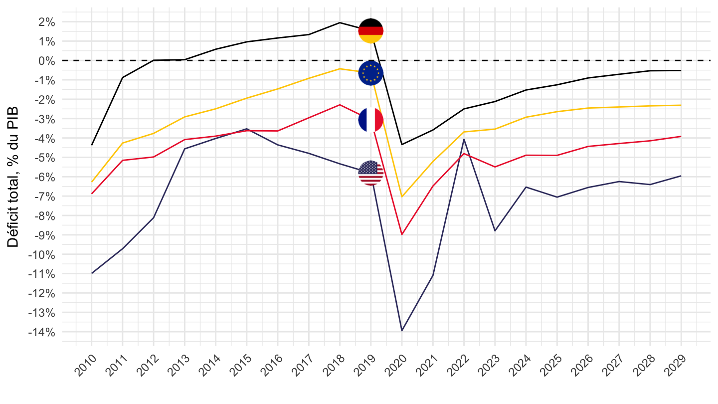
Italy, France, Germany, Spain, United States
1990-
Code
GGXCNL_G01_GDP_PT %>%
  filter(REF_AREA %in% c("IT", "FR", "DE", "ES", "US")) %>%
  left_join(REF_AREA, by = "REF_AREA") %>%
  year_to_date2() %>%
  left_join(colors, by = c("Ref_area" = "country")) %>%
  mutate(OBS_VALUE = OBS_VALUE/100) %>%
  rename(Counterpart_area = Ref_area) %>%
  #filter(date <= as.Date("2021-01-01")) %>%
  ggplot(.) + geom_line(aes(x = date, y = OBS_VALUE, color = color)) +
  theme_minimal() + xlab("") + ylab("Déficit total, % du PIB") +
  scale_color_identity() + add_5flags +
  scale_x_date(breaks = seq(1920, 2100, 5) %>% paste0("-01-01") %>% as.Date,
               labels = date_format("%Y")) +
  scale_y_continuous(breaks = 0.01*seq(-60, 60, 1),
                     labels = scales::percent_format(accuracy = 1)) +
  geom_hline(yintercept = 0, linetype = "dashed", color = "black")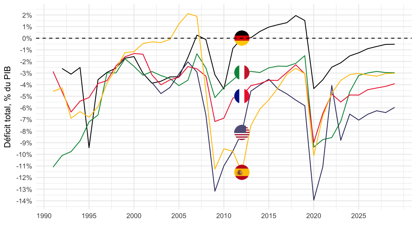
1995-
Code
GGXCNL_G01_GDP_PT %>%
  filter(REF_AREA %in% c("IT", "FR", "DE", "ES", "US")) %>%
  left_join(REF_AREA, by = "REF_AREA") %>%
  year_to_date2() %>%
  left_join(colors, by = c("Ref_area" = "country")) %>%
  mutate(OBS_VALUE = OBS_VALUE/100) %>%
  rename(Counterpart_area = Ref_area) %>%
  filter(date >= as.Date("1995-01-01")) %>%
  ggplot(.) + geom_line(aes(x = date, y = OBS_VALUE, color = color)) +
  theme_minimal() + xlab("") + ylab("Déficit total, % du PIB") +
  scale_color_identity() + add_5flags +
  scale_x_date(breaks = seq(1920, 2100, 5) %>% paste0("-01-01") %>% as.Date,
               labels = date_format("%Y")) +
  scale_y_continuous(breaks = 0.01*seq(-60, 60, 1),
                     labels = scales::percent_format(accuracy = 1)) +
  geom_hline(yintercept = 0, linetype = "dashed", color = "black")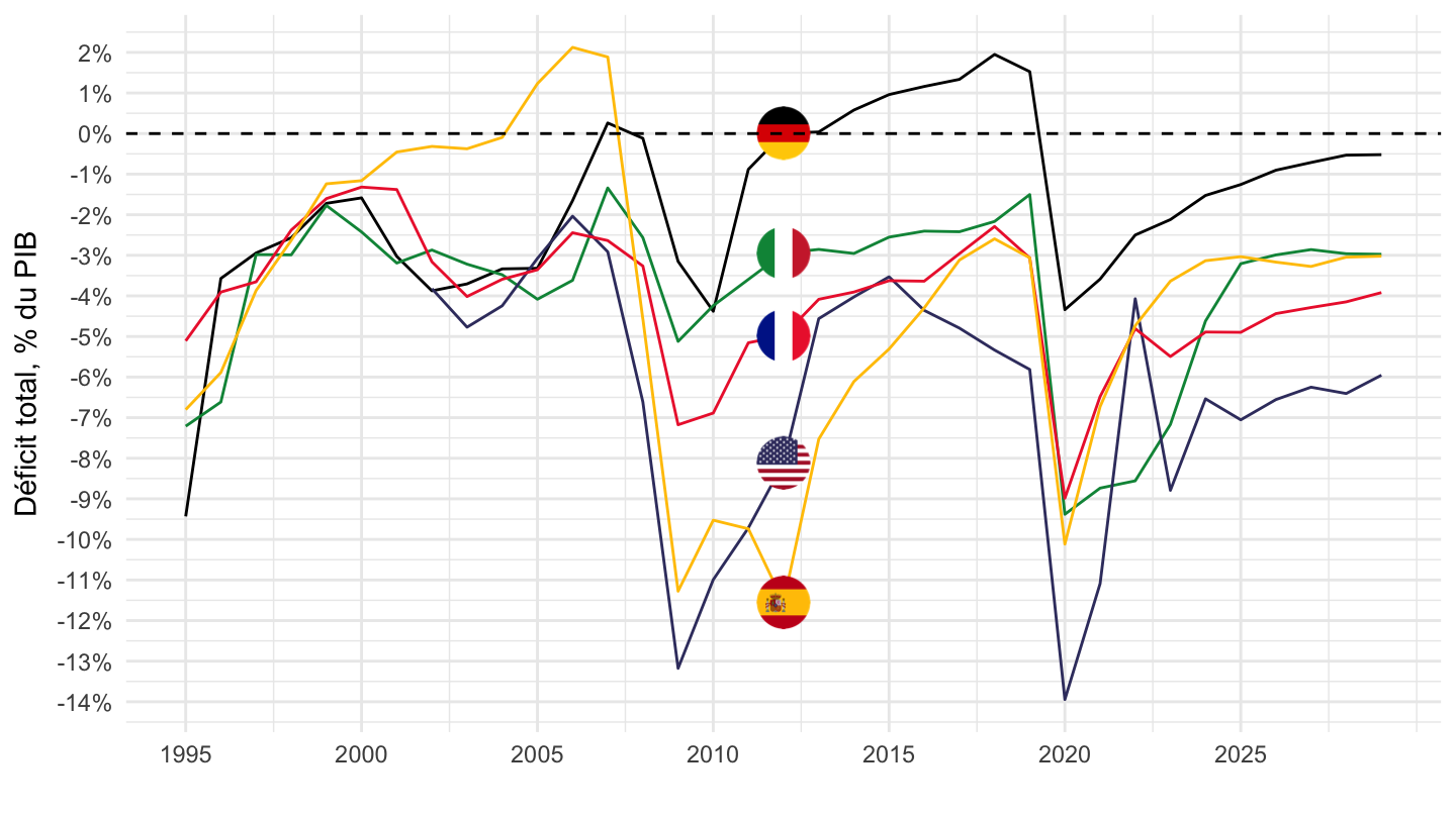
2005-
Code
GGXCNL_G01_GDP_PT %>%
  filter(REF_AREA %in% c("IT", "FR", "DE", "ES", "US")) %>%
  left_join(REF_AREA, by = "REF_AREA") %>%
  year_to_date2() %>%
  left_join(colors, by = c("Ref_area" = "country")) %>%
  mutate(OBS_VALUE = OBS_VALUE/100) %>%
  rename(Counterpart_area = Ref_area) %>%
  filter(date >= as.Date("2005-01-01")) %>%
  ggplot(.) + geom_line(aes(x = date, y = OBS_VALUE, color = color)) +
  theme_minimal() + xlab("") + ylab("Déficit total, % du PIB") +
  scale_color_identity() + add_5flags +
  scale_x_date(breaks = seq(1920, 2100, 2) %>% paste0("-01-01") %>% as.Date,
               labels = date_format("%Y")) +
  scale_y_continuous(breaks = 0.01*seq(-60, 60, 1),
                     labels = scales::percent_format(accuracy = 1)) +
  geom_hline(yintercept = 0, linetype = "dashed", color = "black")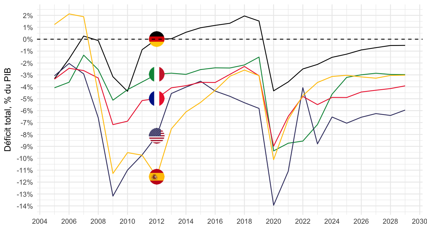
2010-
Code
GGXCNL_G01_GDP_PT %>%
  filter(REF_AREA %in% c("IT", "FR", "DE", "ES", "US")) %>%
  left_join(REF_AREA, by = "REF_AREA") %>%
  year_to_date2() %>%
  left_join(colors, by = c("Ref_area" = "country")) %>%
  mutate(OBS_VALUE = OBS_VALUE/100) %>%
  rename(Counterpart_area = Ref_area) %>%
  filter(date >= as.Date("2010-01-01")) %>%
  ggplot(.) + geom_line(aes(x = date, y = OBS_VALUE, color = color)) +
  theme_minimal() + xlab("") + ylab("Déficit total, % du PIB") +
  scale_color_identity() + add_5flags +
  scale_x_date(breaks = seq(1920, 2100, 2) %>% paste0("-01-01") %>% as.Date,
               labels = date_format("%Y")) +
  scale_y_continuous(breaks = 0.01*seq(-60, 60, 1),
                     labels = scales::percent_format(accuracy = 1)) +
  geom_hline(yintercept = 0, linetype = "dashed", color = "black")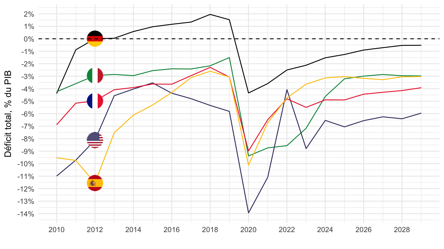
2017-
Code
GGXCNL_G01_GDP_PT %>%
  filter(REF_AREA %in% c("IT", "FR", "DE", "ES", "US", "U2")) %>%
  left_join(REF_AREA, by = "REF_AREA") %>%
  mutate(Ref_area = ifelse(REF_AREA == "U2", "Europe", Ref_area)) %>%
  year_to_date2() %>%
  left_join(colors, by = c("Ref_area" = "country")) %>%
  mutate(OBS_VALUE = OBS_VALUE/100) %>%
  rename(Counterpart_area = Ref_area) %>%
  filter(date >= as.Date("2017-01-01")) %>%
  ggplot(.) + geom_line(aes(x = date, y = OBS_VALUE, color = color)) +
  theme_minimal() + xlab("") + ylab("Déficit total, % du PIB") +
  scale_color_identity() + add_6flags +
  scale_x_date(breaks = seq(1920, 2100, 1) %>% paste0("-01-01") %>% as.Date,
               labels = date_format("%Y")) +
  scale_y_continuous(breaks = 0.01*seq(-60, 60, 1),
                     labels = scales::percent_format(accuracy = 1)) +
  geom_hline(yintercept = 0, linetype = "dashed", color = "black")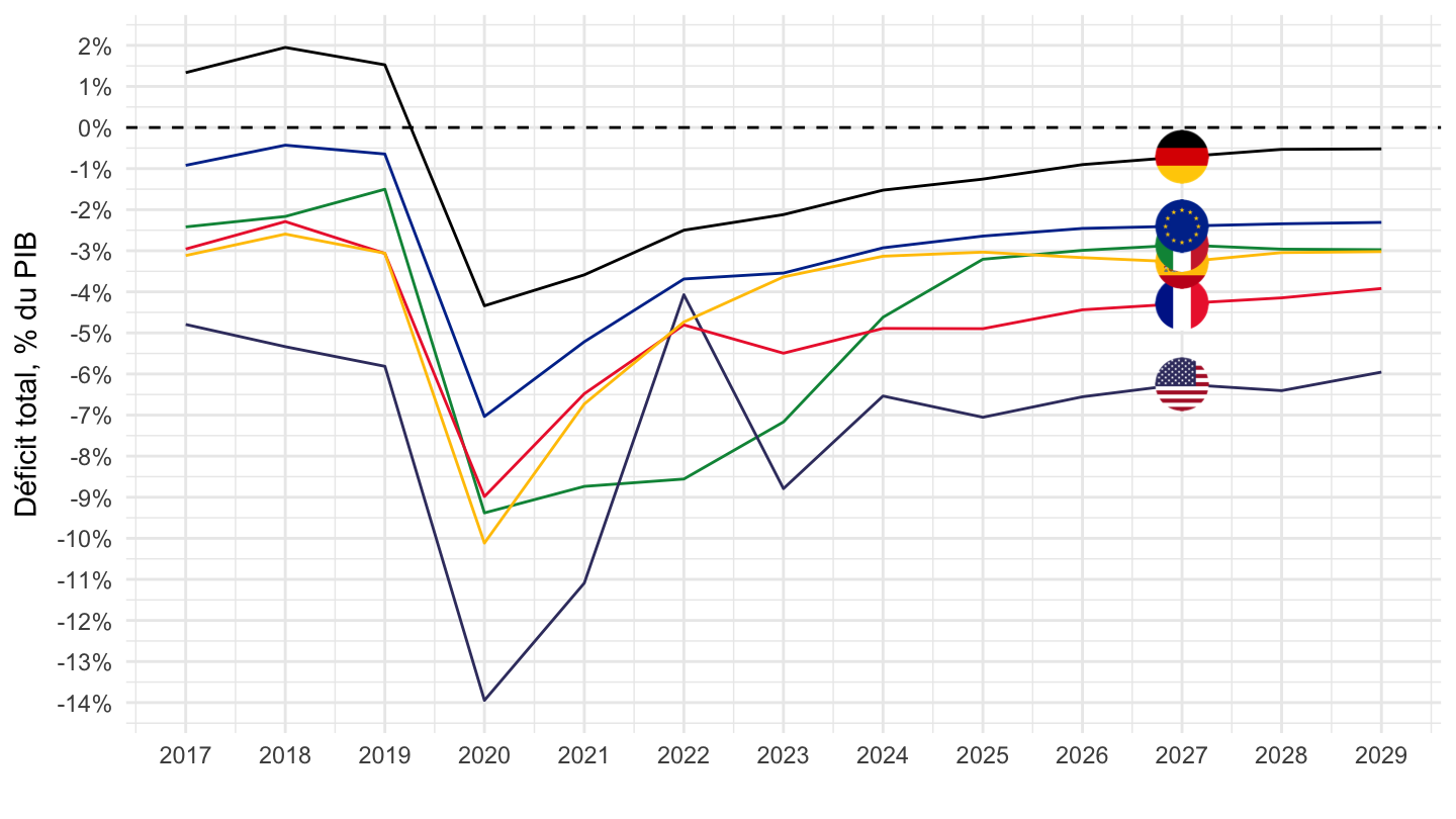
1995-2021
Code
GGXCNL_G01_GDP_PT %>%
  filter(REF_AREA %in% c("IT", "FR", "DE", "ES", "US")) %>%
  left_join(REF_AREA, by = "REF_AREA") %>%
  year_to_date2() %>%
  left_join(colors, by = c("Ref_area" = "country")) %>%
  mutate(OBS_VALUE = OBS_VALUE/100) %>%
  rename(Counterpart_area = Ref_area) %>%
  filter(date <= as.Date("2021-01-01"),
         date >= as.Date("1995-01-01")) %>%
  ggplot(.) + geom_line(aes(x = date, y = OBS_VALUE, color = color)) +
  theme_minimal() + xlab("") + ylab("Déficit total, % du PIB") +
  scale_color_identity() + add_5flags +
  scale_x_date(breaks = seq(1920, 2100, 5) %>% paste0("-01-01") %>% as.Date,
               labels = date_format("%Y")) +
  scale_y_continuous(breaks = 0.01*seq(-60, 60, 1),
                     labels = scales::percent_format(accuracy = 1)) +
  geom_hline(yintercept = 0, linetype = "dashed", color = "black")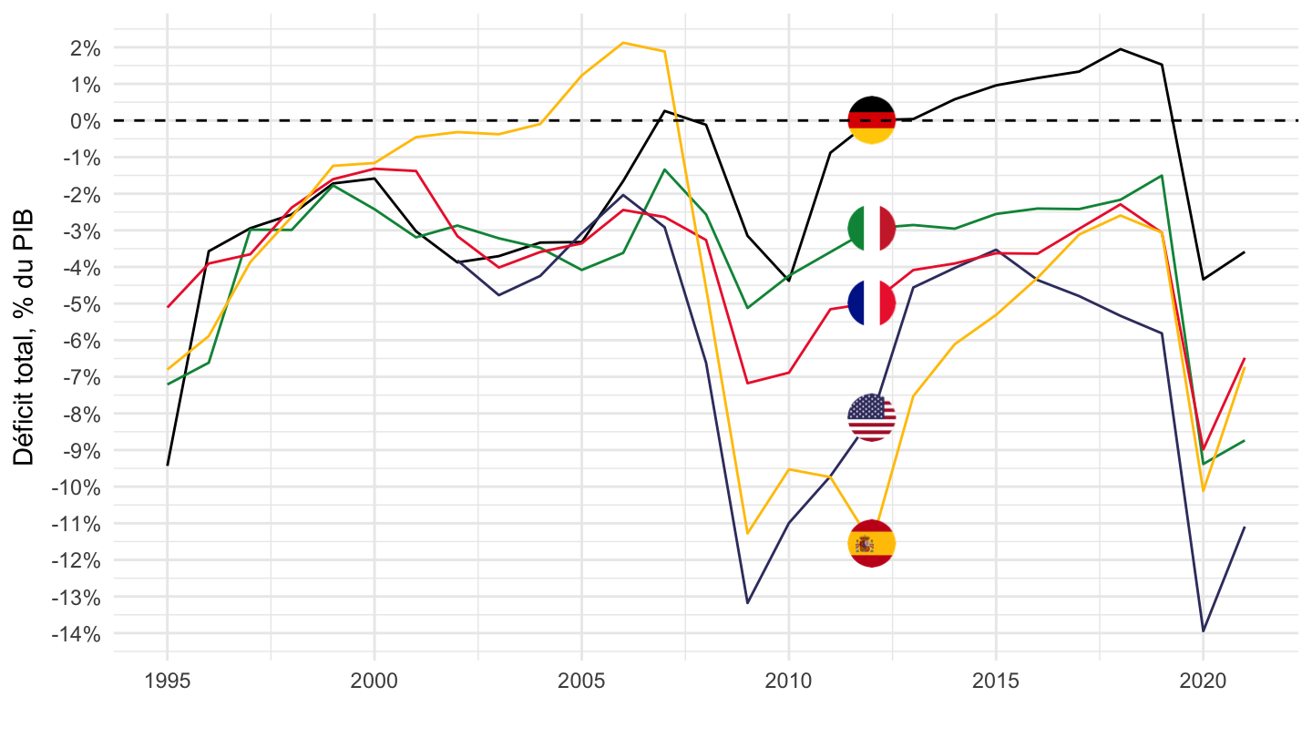
France, Germany, United States, Euro area
All
Code
GGXCNL_G01_GDP_PT %>%
  filter(REF_AREA %in% c("FR", "DE", "US", "U2")) %>%
  left_join(REF_AREA, by = "REF_AREA") %>%
  year_to_date2() %>%
  mutate(Ref_area = ifelse(REF_AREA == "U2", "Europe", Ref_area)) %>%
  left_join(colors, by = c("Ref_area" = "country")) %>%
  mutate(OBS_VALUE = OBS_VALUE/100) %>%
  rename(Counterpart_area = Ref_area) %>%
  #filter(date <= as.Date("2021-01-01")) %>%
  mutate(color = ifelse(REF_AREA == "U2", color2, color)) %>%
  ggplot(.) + geom_line(aes(x = date, y = OBS_VALUE, color = color)) +
  theme_minimal() + xlab("") + ylab("Total Deficit, % of GDP") +
  scale_color_identity() + add_4flags +
  scale_x_date(breaks = seq(1920, 2100, 2) %>% paste0("-01-01") %>% as.Date,
               labels = date_format("%Y")) +
  scale_y_continuous(breaks = 0.01*seq(-60, 60, 1),
                     labels = scales::percent_format(accuracy = 1)) +
  geom_hline(yintercept = 0, linetype = "dashed", color = "black")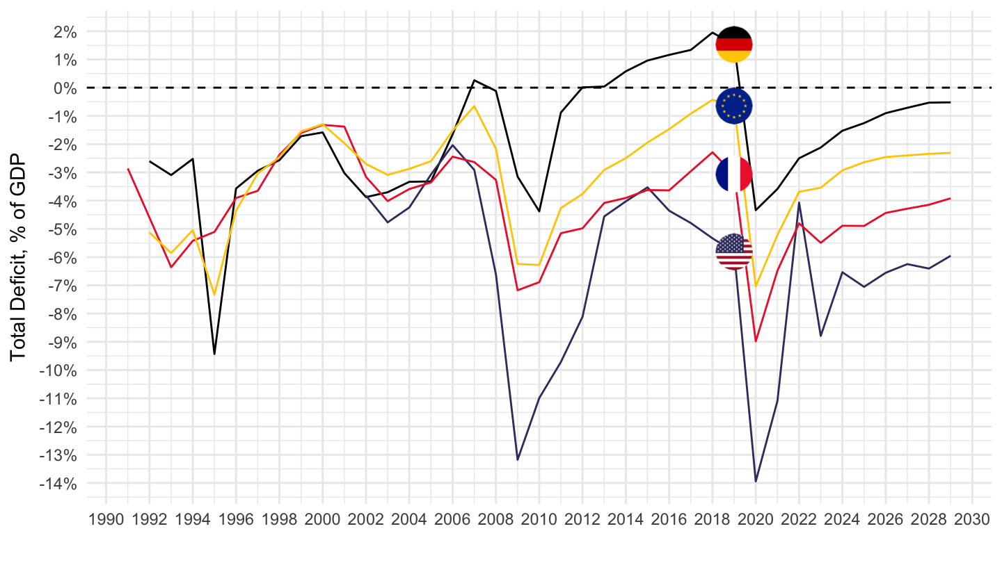
2008-
Code
GGXCNL_G01_GDP_PT %>%
  filter(REF_AREA %in% c("FR", "DE", "US", "U2")) %>%
  left_join(REF_AREA, by = "REF_AREA") %>%
  year_to_date2() %>%
  mutate(Ref_area = ifelse(REF_AREA == "U2", "Europe", Ref_area)) %>%
  left_join(colors, by = c("Ref_area" = "country")) %>%
  mutate(OBS_VALUE = OBS_VALUE/100) %>%
  rename(Counterpart_area = Ref_area) %>%
  filter(date >= as.Date("2008-01-01")) %>%
  mutate(color = ifelse(REF_AREA == "U2", color2, color)) %>%
  ggplot(.) + geom_line(aes(x = date, y = OBS_VALUE, color = color)) +
  theme_minimal() + xlab("") + ylab("Total Deficit, % of GDP") +
  scale_color_identity() + add_4flags +
  scale_x_date(breaks = seq(1920, 2100, 2) %>% paste0("-01-01") %>% as.Date,
               labels = date_format("%Y")) +
  scale_y_continuous(breaks = 0.01*seq(-60, 60, 1),
                     labels = scales::percent_format(accuracy = 1)) +
  geom_hline(yintercept = 0, linetype = "dashed", color = "black")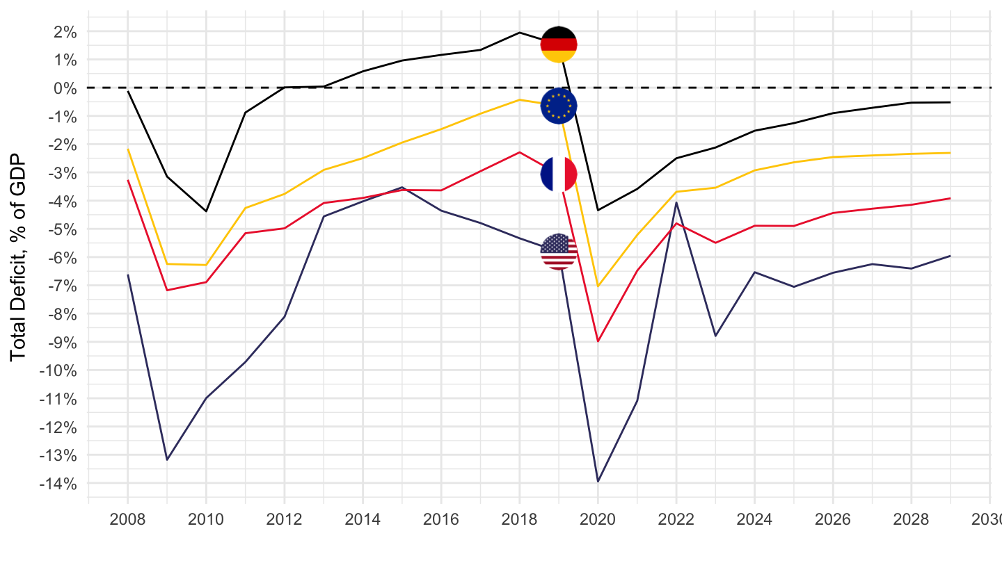
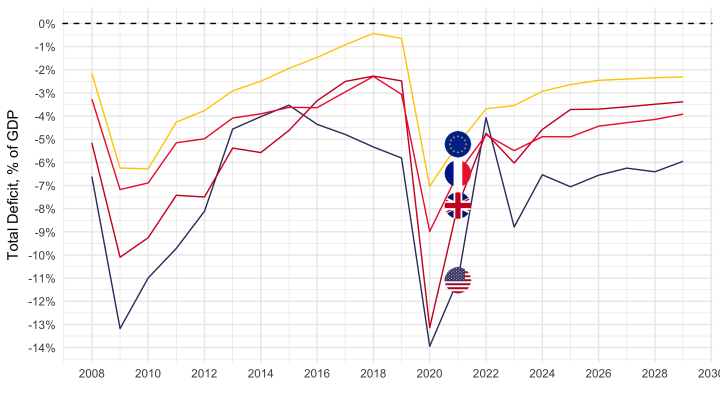
France, United Kingdom, United States, Euro area
All
Code
GGXCNL_G01_GDP_PT %>%
  filter(REF_AREA %in% c("FR", "GB", "US", "U2")) %>%
  left_join(REF_AREA, by = "REF_AREA") %>%
  year_to_date2() %>%
  mutate(Ref_area = ifelse(REF_AREA == "U2", "Europe", Ref_area)) %>%
  left_join(colors, by = c("Ref_area" = "country")) %>%
  mutate(OBS_VALUE = OBS_VALUE/100) %>%
  rename(Counterpart_area = Ref_area) %>%
  #filter(date <= as.Date("2021-01-01")) %>%
  mutate(color = ifelse(REF_AREA == "U2", color2, color)) %>%
  ggplot(.) + geom_line(aes(x = date, y = OBS_VALUE, color = color)) +
  theme_minimal() + xlab("") + ylab("Total Deficit, % of GDP") +
  scale_color_identity() + add_4flags +
  scale_x_date(breaks = seq(1920, 2100, 2) %>% paste0("-01-01") %>% as.Date,
               labels = date_format("%Y")) +
  scale_y_continuous(breaks = 0.01*seq(-60, 60, 1),
                     labels = scales::percent_format(accuracy = 1)) +
  geom_hline(yintercept = 0, linetype = "dashed", color = "black")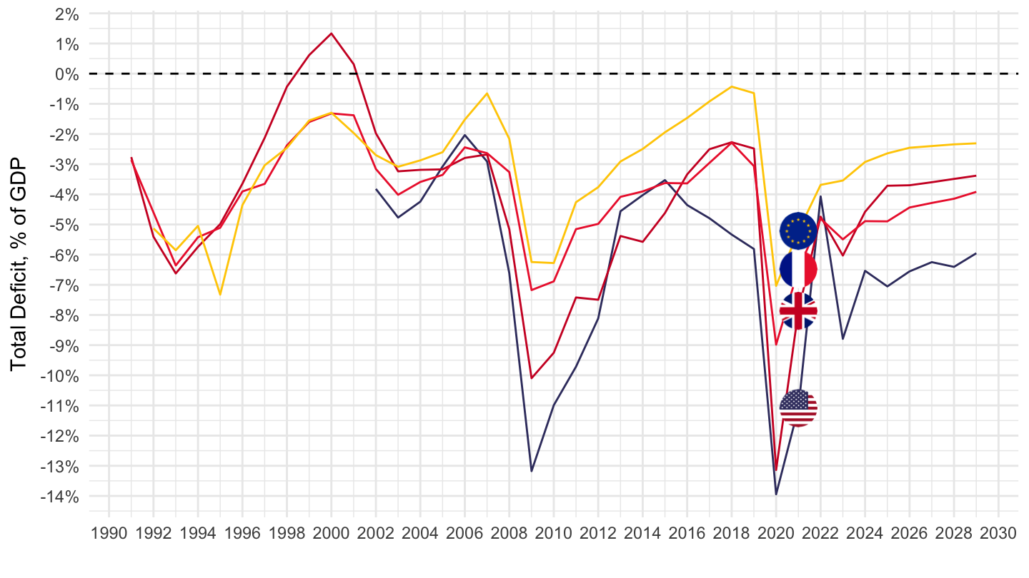
2008-
Code
GGXCNL_G01_GDP_PT %>%
  filter(REF_AREA %in% c("FR", "GB", "US", "U2")) %>%
  left_join(REF_AREA, by = "REF_AREA") %>%
  year_to_date2() %>%
  mutate(Ref_area = ifelse(REF_AREA == "U2", "Europe", Ref_area)) %>%
  left_join(colors, by = c("Ref_area" = "country")) %>%
  mutate(OBS_VALUE = OBS_VALUE/100) %>%
  rename(Counterpart_area = Ref_area) %>%
  filter(date >= as.Date("2008-01-01")) %>%
  mutate(color = ifelse(REF_AREA == "U2", color2, color)) %>%
  ggplot(.) + geom_line(aes(x = date, y = OBS_VALUE, color = color)) +
  theme_minimal() + xlab("") + ylab("Total Deficit, % of GDP") +
  scale_color_identity() + add_4flags +
  scale_x_date(breaks = seq(1920, 2100, 2) %>% paste0("-01-01") %>% as.Date,
               labels = date_format("%Y")) +
  scale_y_continuous(breaks = 0.01*seq(-60, 60, 1),
                     labels = scales::percent_format(accuracy = 1)) +
  geom_hline(yintercept = 0, linetype = "dashed", color = "black")