Code
GGXWDG_GDP %>%
  group_by(TIME_PERIOD) %>%
  summarise(Nobs = n()) %>%
  arrange(desc(TIME_PERIOD)) %>%
print_table_conditional()Data - IMF
GGXWDG_GDP %>%
group_by(TIME_PERIOD) %>%
summarise(Nobs = n()) %>%
arrange(desc(TIME_PERIOD)) %>%
print_table_conditional()GGXWDG_GDP %>%
year_to_date2() %>%
filter(REF_AREA %in% c("US", "FR", "JP", "DE", "IT")) %>%
left_join(REF_AREA, by = "REF_AREA") %>%
left_join(colors, by = c("Ref_area" = "country")) %>%
mutate(OBS_VALUE = OBS_VALUE / 100,
Counterpart_area = Ref_area) %>%
ggplot(.) + geom_line(aes(x = date, y = OBS_VALUE, color = color)) +
theme_minimal() + scale_color_identity() + xlab("") + ylab("Government Debt (% of GDP)") +
add_4flags +
theme(legend.position = "none") +
scale_y_continuous(breaks = 0.01*seq(0, 260, 20),
labels = scales::percent_format(accuracy = 1)) +
scale_x_date(breaks = as.Date(paste0(seq(1700, 2100, 20), "-01-01")),
labels = date_format("%Y"))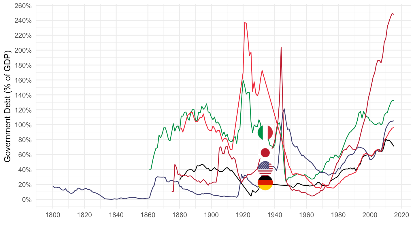
GGXWDG_GDP %>%
  filter(TIME_PERIOD == "2015") %>%
  left_join(REF_AREA, by = "REF_AREA") %>%
  mutate(OBS_VALUE = round(OBS_VALUE) %>% paste0(., " %")) %>%
  select(REF_AREA, Ref_area, `Public Debt (2015)` = OBS_VALUE) %>%
  as.tibble %>%
{if (is_html_output()) datatable(., filter = 'top', rownames = F) else .}GGXWDG_GDP %>%
filter(REF_AREA %in% c("AT")) %>%
year_to_date2() %>%
ggplot(.) + geom_line(aes(x = date, y = OBS_VALUE / 100)) + theme_minimal() +
scale_y_continuous(breaks = 0.01*seq(0, 260, 10),
labels = scales::percent_format(accuracy = 1)) +
scale_x_date(breaks = as.Date(paste0(seq(1700, 2100, 20), "-01-01")),
labels = date_format("%Y")) +
xlab("") + ylab("Government Debt (% of GDP)")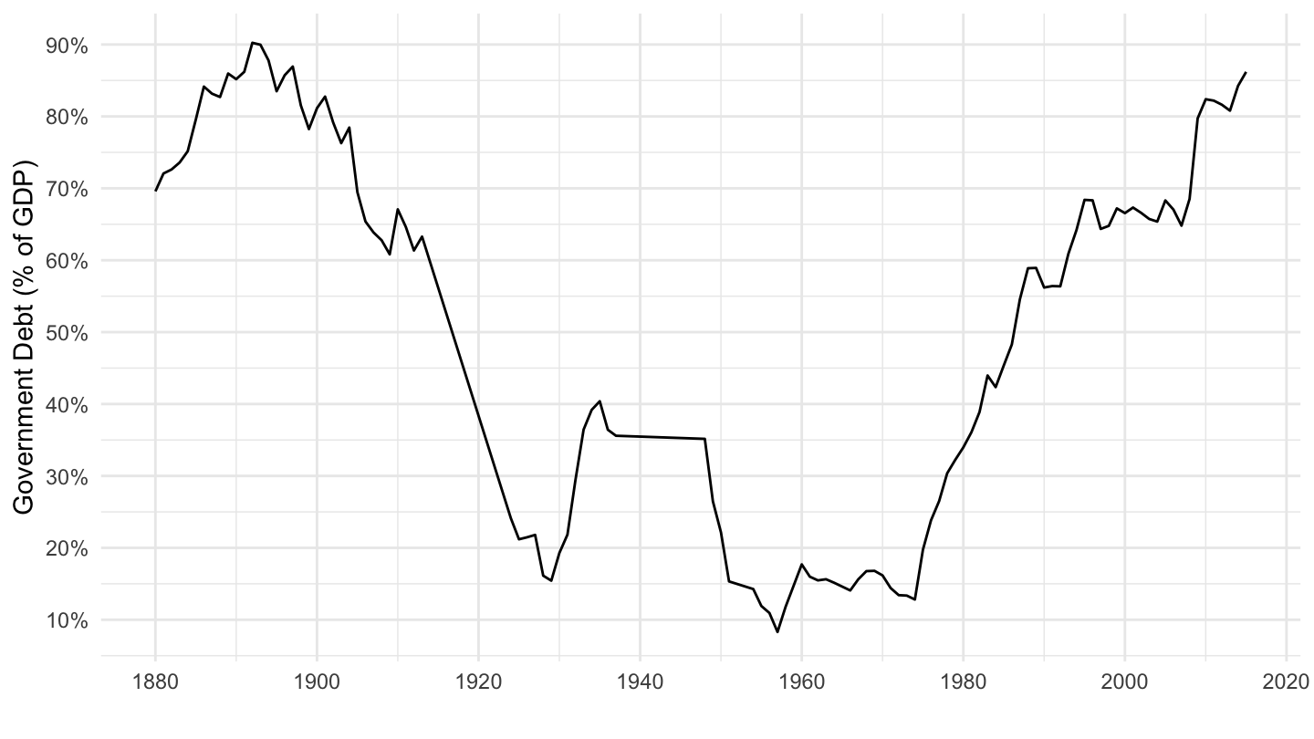
GGXWDG_GDP %>%
  year_to_date2() %>%
  filter(REF_AREA %in% c("SG")) %>%
  ggplot(.) + geom_line(aes(x = date, y = OBS_VALUE / 100)) + theme_minimal() +
  scale_y_continuous(breaks = 0.01*seq(0, 260, 10),
                     labels = scales::percent_format(accuracy = 1)) +
  scale_x_date(breaks = as.Date(paste0(seq(1700, 2100, 5), "-01-01")),
               labels = date_format("%Y")) +
  xlab("") + ylab("Government Debt (% of GDP)")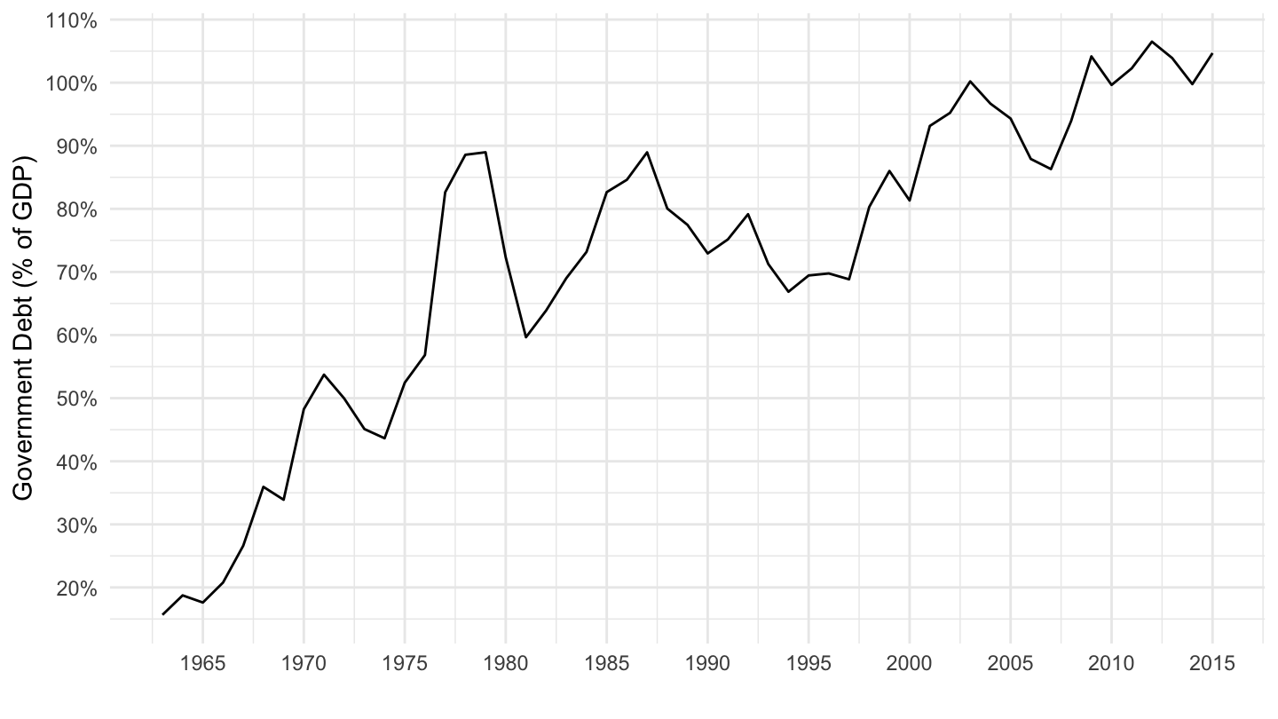
GGXWDG_GDP %>%
  year_to_date2() %>%
  filter(REF_AREA %in% c("US", "GB")) %>%
  left_join(REF_AREA, by = "REF_AREA") %>%
  ggplot(.) + geom_line(aes(x = date, y = OBS_VALUE / 100, color = Ref_area)) + theme_minimal() +
  scale_color_manual(values = c("#6E82B5", "#B22234")) +
  geom_image(data = . %>%
               filter(date == as.Date("1840-01-01")) %>%
               mutate(date = as.Date("1840-01-01"),
                      image = paste0("../../icon/flag/round/", str_to_lower(gsub(" ", "-", Ref_area)), ".png")),
             aes(x = date, y = OBS_VALUE/100, image = image), asp = 1.5) +
  theme(legend.position = "none") +
  scale_y_continuous(breaks = 0.01*seq(0, 260, 20),
                     labels = scales::percent_format(accuracy = 1)) +
  scale_x_date(breaks = as.Date(paste0(seq(1700, 2100, 20), "-01-01")),
               labels = date_format("%Y")) +
  xlab("") + ylab("Government Debt (% of GDP)")
GGXWDG_GDP %>%
  year_to_date2() %>%
  filter(REF_AREA %in% c("US", "GB", "FR")) %>%
  group_by(REF_AREA) %>%
  mutate(year = year(date)) %>%
  complete(date = seq.Date(min(date), max(date), by = "year")) %>%
  left_join(REF_AREA, by = "REF_AREA") %>%
  ggplot(.) + geom_line(aes(x = date, y = OBS_VALUE / 100, color = Ref_area)) + theme_minimal() +
  scale_color_manual(values = c("#000000", "#6E82B5", "#B22234")) +
  geom_image(data = . %>%
               filter(date == as.Date("1895-01-01")) %>%
               mutate(date = as.Date("1895-01-01"),
                      image = paste0("../../icon/flag/round/", str_to_lower(gsub(" ", "-", Ref_area)), ".png")),
             aes(x = date, y = OBS_VALUE/100, image = image), asp = 1.5) +
  theme(legend.position = "none") +
  scale_y_continuous(breaks = 0.01*seq(0, 260, 20),
                     labels = scales::percent_format(accuracy = 1)) +
  scale_x_date(breaks = as.Date(paste0(seq(1700, 2100, 20), "-01-01")),
               labels = date_format("%Y")) +
  xlab("") + ylab("Government Debt (% of GDP)")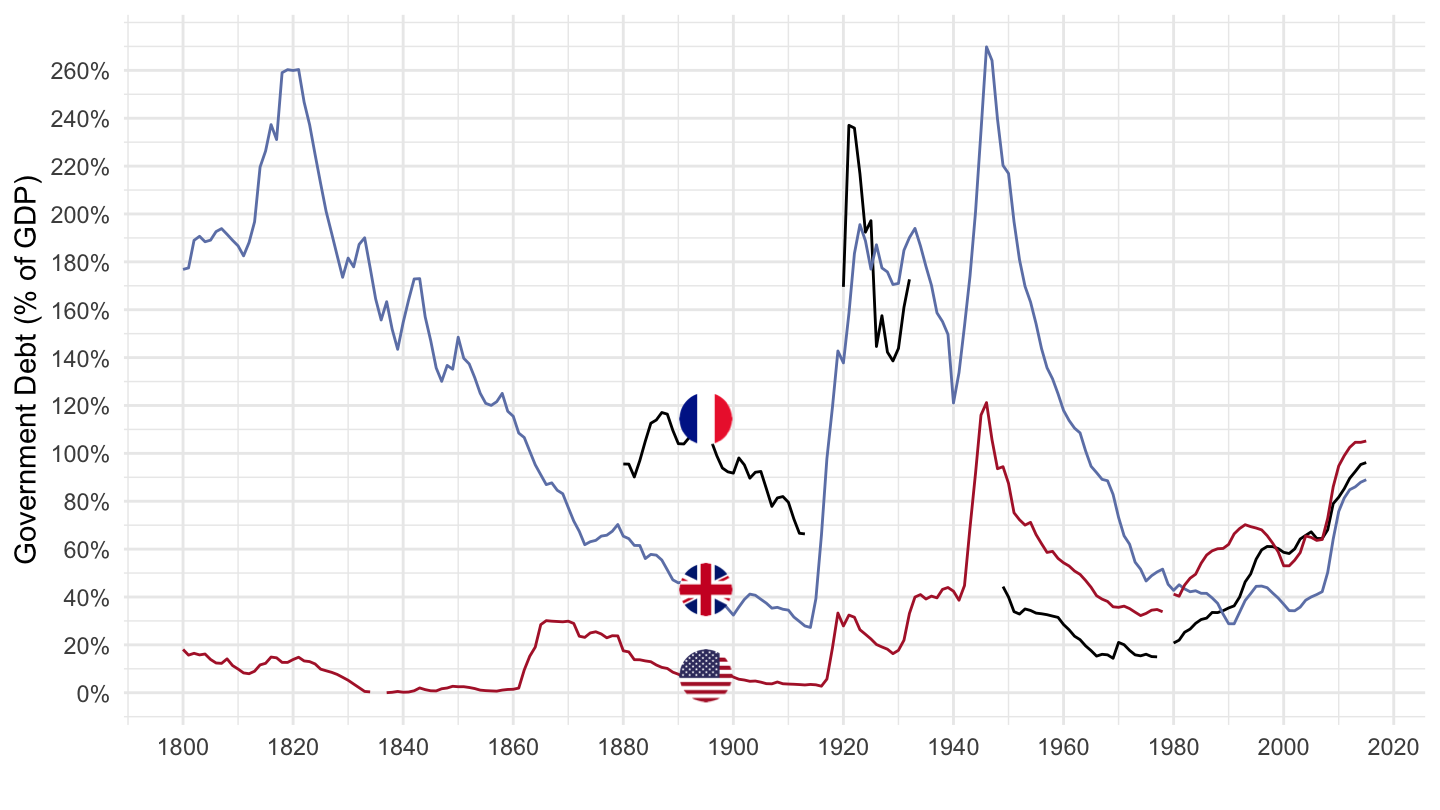
GGXWDG_GDP %>%
  year_to_date2() %>%
  filter(REF_AREA %in% c("US", "GB")) %>%
  bind_rows(gfd_france) %>%
  left_join(REF_AREA, by = "REF_AREA") %>%
  ggplot(.) + geom_line(aes(x = date, y = OBS_VALUE / 100, color = Ref_area)) + theme_minimal() +
  scale_color_manual(values = c("#002395", "#6E82B5", "#B22234")) +
  geom_image(data = . %>%
               filter(date == as.Date("1895-01-01")) %>%
               mutate(date = as.Date("1895-01-01"),
                      image = paste0("../../icon/flag/round/", str_to_lower(gsub(" ", "-", Ref_area)), ".png")),
             aes(x = date, y = OBS_VALUE/100, image = image), asp = 1.5) +
  theme(legend.position = "none") +
  scale_y_continuous(breaks = 0.01*seq(0, 260, 20),
                     labels = scales::percent_format(accuracy = 1)) +
  scale_x_date(breaks = as.Date(paste0(seq(1700, 2100, 20), "-01-01")),
               labels = date_format("%Y")) +
  xlab("") + ylab("Government Debt (% of GDP)")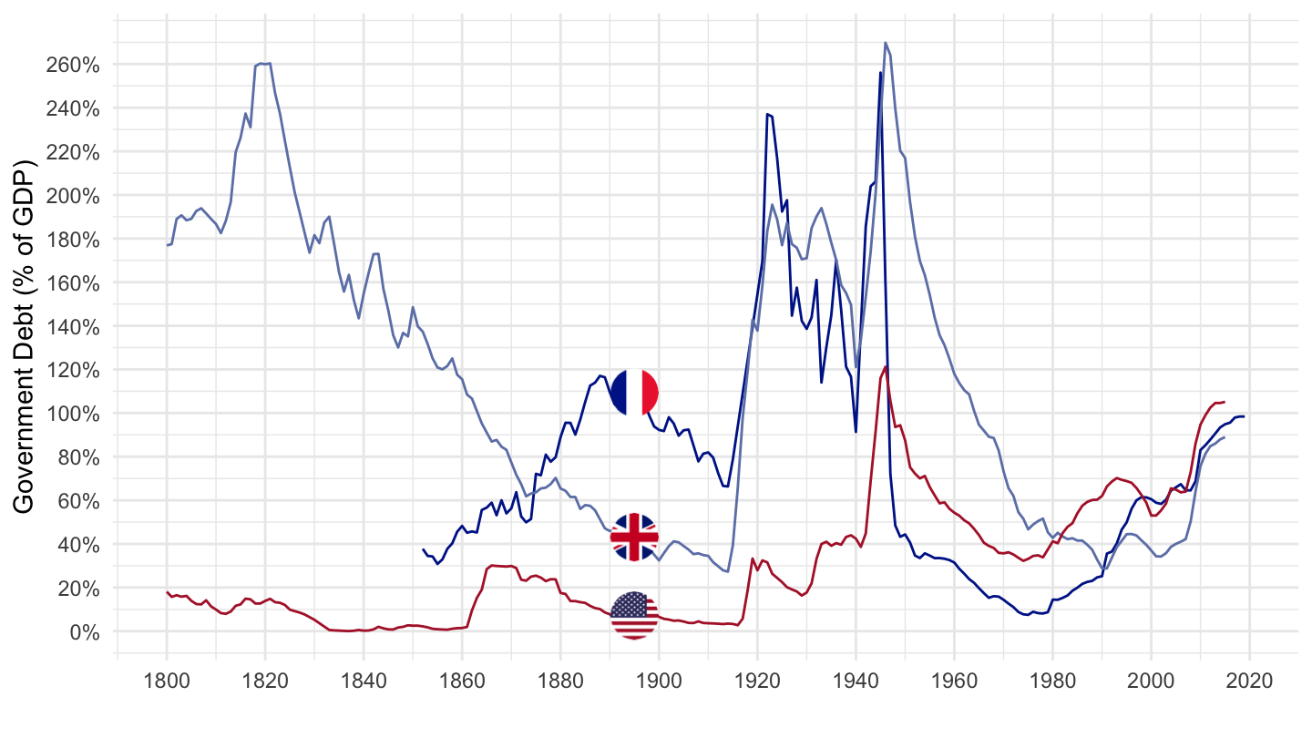
GGXWDG_GDP %>%
  year_to_date2() %>%
  filter(REF_AREA %in% c("US")) %>%
  bind_rows(gfd_france) %>%
  bind_rows(gfd_japan) %>%
  left_join(REF_AREA, by = "REF_AREA") %>%
  left_join(colors, by = c("Ref_area" = "country")) %>%
  mutate(OBS_VALUE = OBS_VALUE / 100,
         Counterpart_area = Ref_area) %>%
  ggplot(.) + geom_line(aes(x = date, y = OBS_VALUE, color = color)) +
  theme_minimal() + scale_color_identity() + xlab("") + ylab("Government Debt (% of GDP)") +
  add_3flags +
  theme(legend.position = "none") +
  scale_y_continuous(breaks = 0.01*seq(0, 260, 20),
                     labels = scales::percent_format(accuracy = 1)) +
  scale_x_date(breaks = as.Date(paste0(seq(1700, 2100, 20), "-01-01")),
               labels = date_format("%Y"))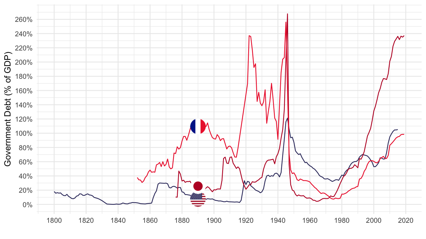
GGXWDG_GDP %>%
  year_to_date2() %>%
  filter(REF_AREA %in% c("US", "GB")) %>%
  bind_rows(gfd_france) %>%
  bind_rows(gfd_japan) %>%
  bind_rows(gfd_italy) %>%
  left_join(REF_AREA, by = "REF_AREA") %>%
  ggplot(.) + geom_line(aes(x = date, y = OBS_VALUE / 100, color = Ref_area, linetype = Ref_area)) +
  theme_minimal() +
  scale_color_manual(values = c("#000000", "#009246", "#BC002D", "#6E82B5", "#B22234")) +
  scale_linetype_manual(values = c("solid", "solid", "longdash","solid",  "solid")) +
  geom_image(data = . %>%
               filter(date == as.Date("1887-01-01")) %>%
               mutate(date = as.Date("1887-01-01"),
                      image = paste0("../../icon/flag/round/", str_to_lower(gsub(" ", "-", Ref_area)), ".png")),
             aes(x = date, y = OBS_VALUE/100, image = image), asp = 1.5) +
  theme(legend.position = c(0.5, 0.97),
        legend.title = element_blank(),
        legend.direction = "horizontal") +
  scale_y_continuous(breaks = 0.01*seq(0, 260, 20),
                     labels = scales::percent_format(accuracy = 1)) +
  scale_x_date(breaks = as.Date(paste0(seq(1700, 2100, 20), "-01-01")),
               labels = date_format("%Y")) +
  xlab("") + ylab("Government Debt (% of GDP)")
GGXWDG_GDP %>%
  year_to_date2() %>%
  filter(REF_AREA %in% c("US", "GB")) %>%
  bind_rows(gfd_france) %>%
  bind_rows(gfd_japan) %>%
  bind_rows(gfd_italy) %>%
  left_join(REF_AREA, by = "REF_AREA") %>%
  ggplot(.) + geom_line(aes(x = date, y = OBS_VALUE / 100, color = Ref_area, linetype = Ref_area)) +
  theme_minimal() +
  scale_color_manual(values = c("#000000", "#009246", "#BC002D", "#6E82B5", "#B22234")) +
  scale_linetype_manual(values = c("solid", "solid","longdash","solid",  "solid")) +
  geom_image(data = . %>%
               filter(date == as.Date("1887-01-01")) %>%
               mutate(date = as.Date("1887-01-01"),
                      image = paste0("../../icon/flag/round/", str_to_lower(gsub(" ", "-", Ref_area)), ".png")),
             aes(x = date, y = OBS_VALUE/100, image = image), asp = 1.5) +
  theme(legend.position = c(0.5, 0.97),
        legend.title = element_blank(),
        legend.direction = "horizontal") +
  scale_y_continuous(breaks = 0.01*seq(0, 260, 20),
                     labels = scales::percent_format(accuracy = 1)) +
  scale_x_date(breaks = as.Date(paste0(seq(1700, 2100, 20), "-01-01")),
               labels = date_format("%Y")) +
  xlab("") + ylab("Government Debt (% of GDP)")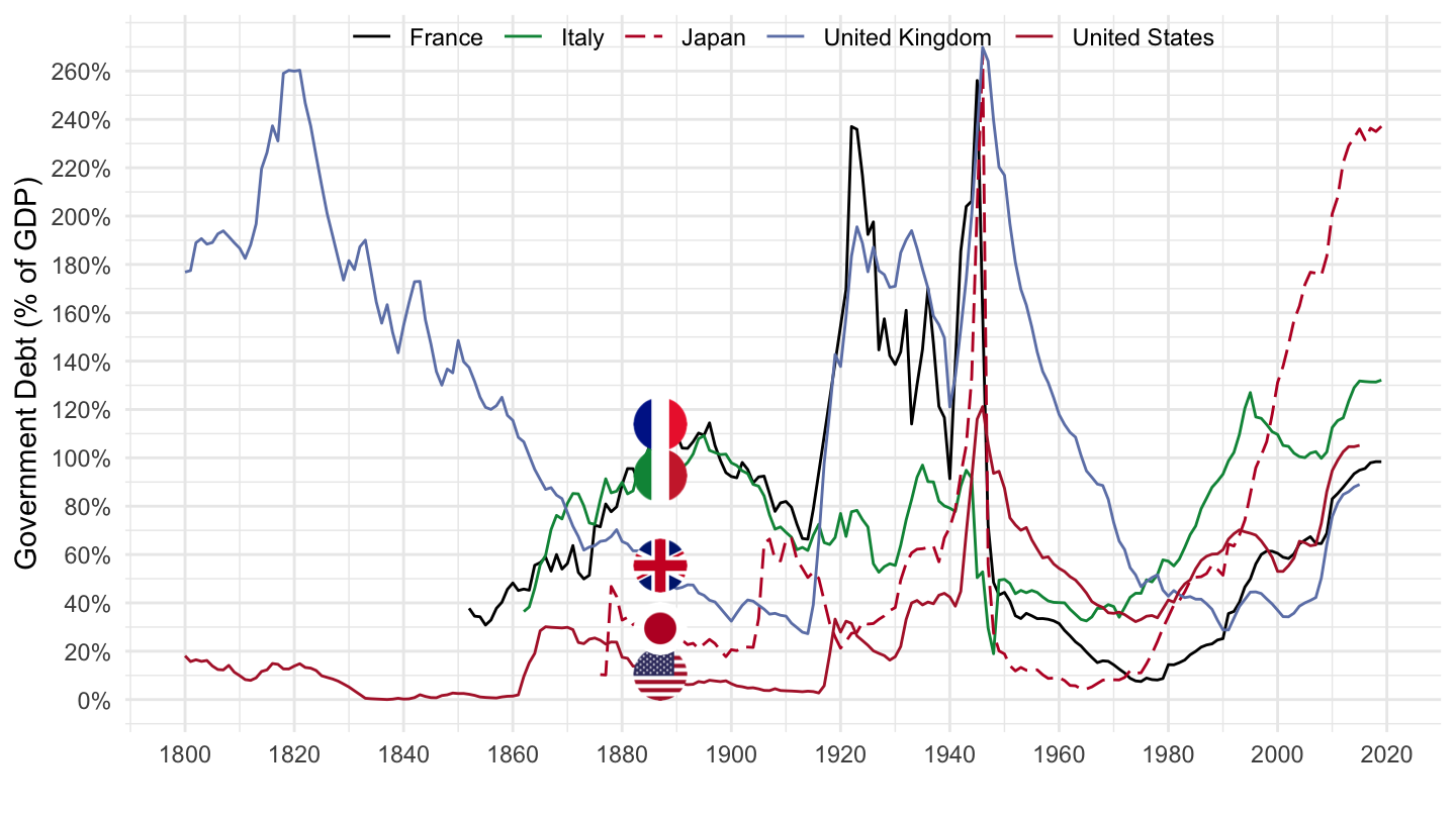
GGXWDG_GDP %>%
  year_to_date2() %>%
  filter(REF_AREA %in% c("US", "GB")) %>%
  bind_rows(gfd_france) %>%
  bind_rows(gfd_japan) %>%
  bind_rows(gfd_italy) %>%
  left_join(REF_AREA, by = "REF_AREA") %>%
  ggplot(.) + geom_line(aes(x = date, y = OBS_VALUE / 100, color = Ref_area, linetype = Ref_area)) +
  theme_minimal() +
  scale_color_manual(values = c("#000000", "#009246", "#BC002D", "#6E82B5", "#B22234")) +
  scale_linetype_manual(values = c("solid", "solid","longdash","solid",  "solid")) +
  geom_image(data = . %>%
               filter(date == as.Date("1887-01-01")) %>%
               mutate(date = as.Date("1887-01-01"),
                      image = paste0("../../icon/flag/round/", str_to_lower(gsub(" ", "-", Ref_area)), ".png")),
             aes(x = date, y = OBS_VALUE/100, image = image), asp = 1.5) +
  theme(legend.position = c(0.5, 0.97),
        legend.title = element_blank(),
        legend.direction = "horizontal") +
  scale_y_continuous(breaks = 0.01*seq(0, 260, 20),
                     labels = scales::percent_format(accuracy = 1)) +
  scale_x_date(breaks = as.Date(paste0(seq(1700, 2100, 20), "-01-01")),
               labels = date_format("%Y")) +
  xlab("") + ylab("Government Debt (% of GDP)")
GGXWDG_GDP %>%
  year_to_date2() %>%
  filter(REF_AREA %in% c("US")) %>%
  ggplot(.) + geom_line(aes(x = date, y = OBS_VALUE / 100)) + theme_minimal() +
  geom_rect(data = nber_recessions,
            aes(xmin = Peak, xmax = Trough, ymin = -Inf, ymax = +Inf),
            fill = 'grey', alpha = 0.5) +
  scale_y_continuous(breaks = 0.01*seq(0, 260, 10),
                     labels = scales::percent_format(accuracy = 1)) +
  scale_x_date(breaks = as.Date(paste0(seq(1700, 2100, 20), "-01-01")),
               labels = date_format("%Y")) +
  xlab("") + ylab("Government Debt (% of GDP)")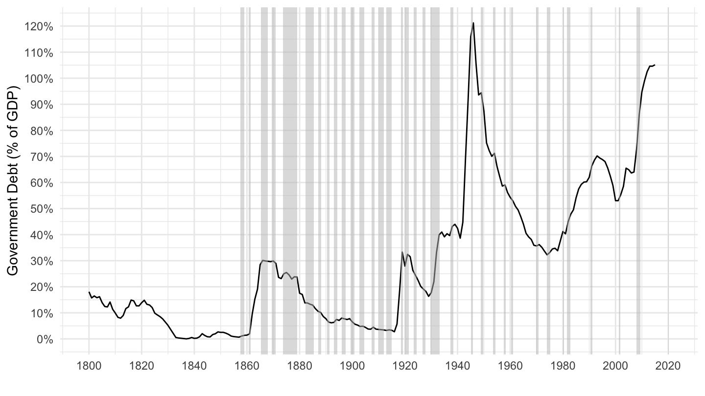
GGXWDG_GDP %>%
  year_to_date2() %>%
  filter(REF_AREA %in% c("GB")) %>%
  ggplot(.) + geom_line(aes(x = date, y = OBS_VALUE / 100)) + theme_minimal() +
  scale_y_continuous(breaks = 0.01*seq(0, 260, 10),
                     labels = scales::percent_format(accuracy = 1)) +
  scale_x_date(breaks = as.Date(paste0(seq(1700, 2100, 20), "-01-01")),
               labels = date_format("%Y")) +
  xlab("") + ylab("Government Debt (% of GDP)")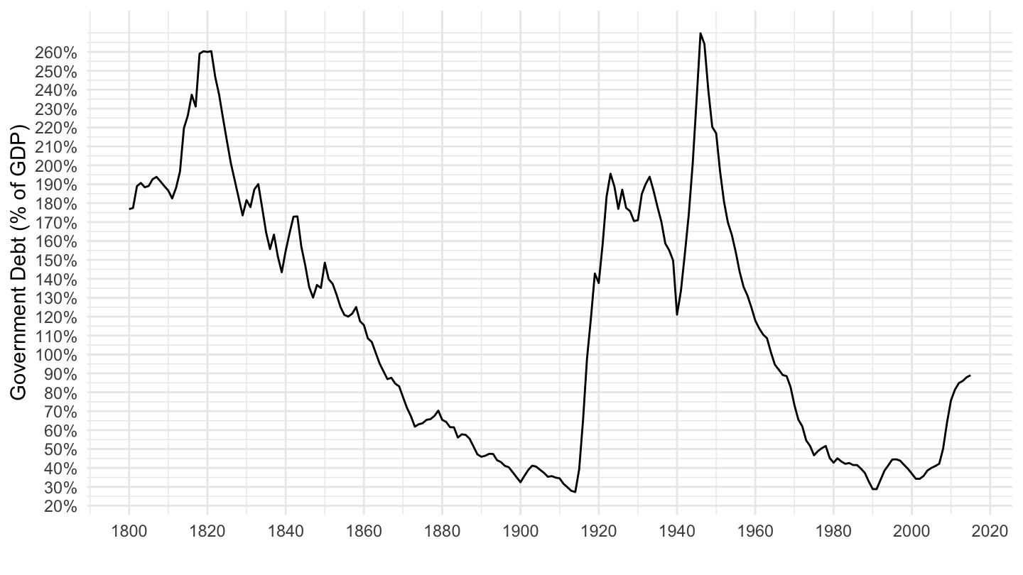
gfd_france %>%
  complete(date = seq.Date(min(date), max(date), by = "year")) %>%
  ggplot(.) + geom_line(aes(x = date, y = OBS_VALUE / 100)) + theme_minimal() +
  scale_y_continuous(breaks = 0.01*seq(0, 260, 10),
                     labels = scales::percent_format(accuracy = 1)) +
  scale_x_date(breaks = as.Date(paste0(seq(1700, 2100, 20), "-01-01")),
               labels = date_format("%Y")) +
  xlab("") + ylab("Government Debt (% of GDP)")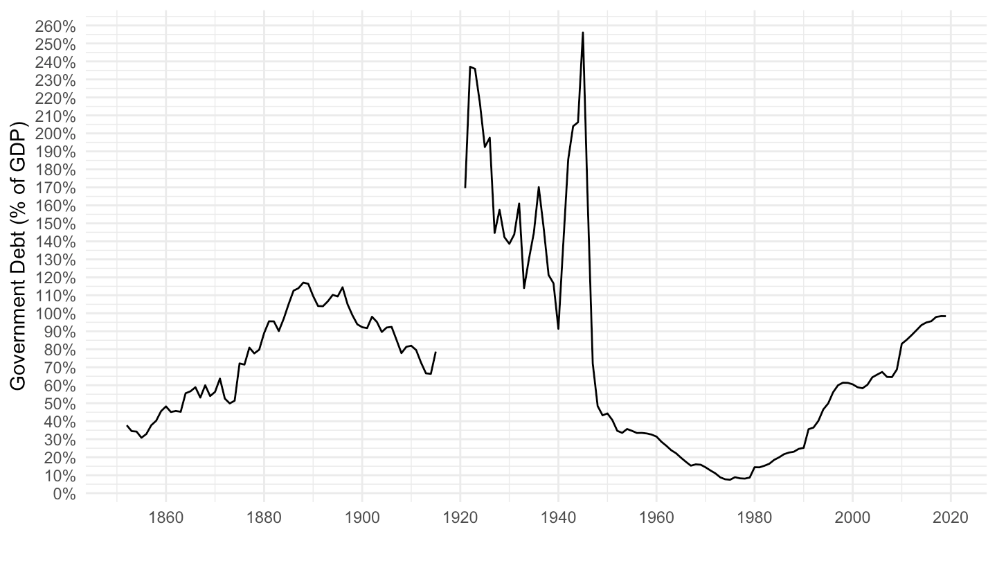
gfd_france %>%
  complete(date = seq.Date(min(date), max(date), by = "year")) %>%
  ggplot(.) + geom_line(aes(x = date, y = OBS_VALUE / 100)) + theme_minimal() +
  scale_y_continuous(breaks = 0.01*seq(0, 260, 10)) +
  scale_x_date(breaks = as.Date(paste0(seq(1700, 2100, 20), "-01-01")),
               labels = date_format("%Y")) +
  xlab("") + ylab("Government Debt (years of GDP)")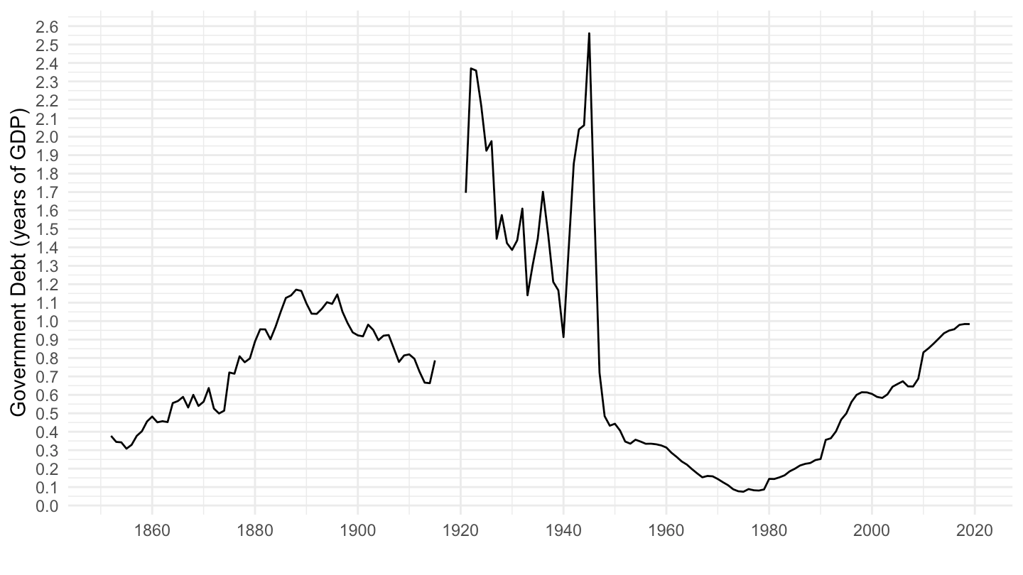
GGXWDG_GDP %>%
  year_to_date2() %>%
  filter(REF_AREA %in% c("FR")) %>%
  complete(date = seq.Date(min(date), max(date), by = "year")) %>%
  ggplot(.) + geom_line(aes(x = date, y = OBS_VALUE / 100)) + theme_minimal() +
  scale_y_continuous(breaks = 0.01*seq(0, 260, 10),
                     labels = scales::percent_format(accuracy = 1)) +
  scale_x_date(breaks = as.Date(paste0(seq(1700, 2100, 20), "-01-01")),
               labels = date_format("%Y")) +
  xlab("") + ylab("Government Debt (% of GDP)")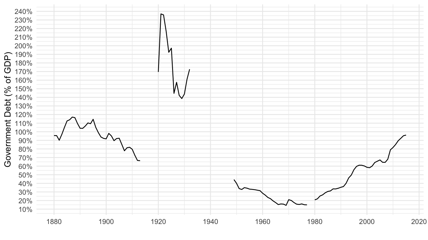
GGXWDG_GDP %>%
  year_to_date2() %>%
  filter(REF_AREA %in% c("FR")) %>%
  complete(date = seq.Date(min(date), max(date), by = "year")) %>%
  ggplot(.) + geom_line(aes(x = date, y = OBS_VALUE / 100)) + theme_minimal() +
  scale_y_continuous(breaks = 0.01*seq(0, 260, 10)) +
  scale_x_date(breaks = as.Date(paste0(seq(1700, 2100, 20), "-01-01")),
               labels = date_format("%Y")) +
  xlab("") + ylab("Government Debt (Years of GDP)")
GGXWDG_GDP %>%
  year_to_date2() %>%
  filter(REF_AREA %in% c("JP")) %>%
  complete(date = seq.Date(min(date), max(date), by = "year")) %>%
  ggplot(.) + geom_line(aes(x = date, y = OBS_VALUE / 100)) + theme_minimal() +
  scale_y_continuous(breaks = 0.01*seq(0, 260, 10),
                     labels = scales::percent_format(accuracy = 1)) +
  scale_x_date(breaks = as.Date(paste0(seq(1700, 2100, 20), "-01-01")),
               labels = date_format("%Y")) +
  xlab("") + ylab("Government Debt (% of GDP)")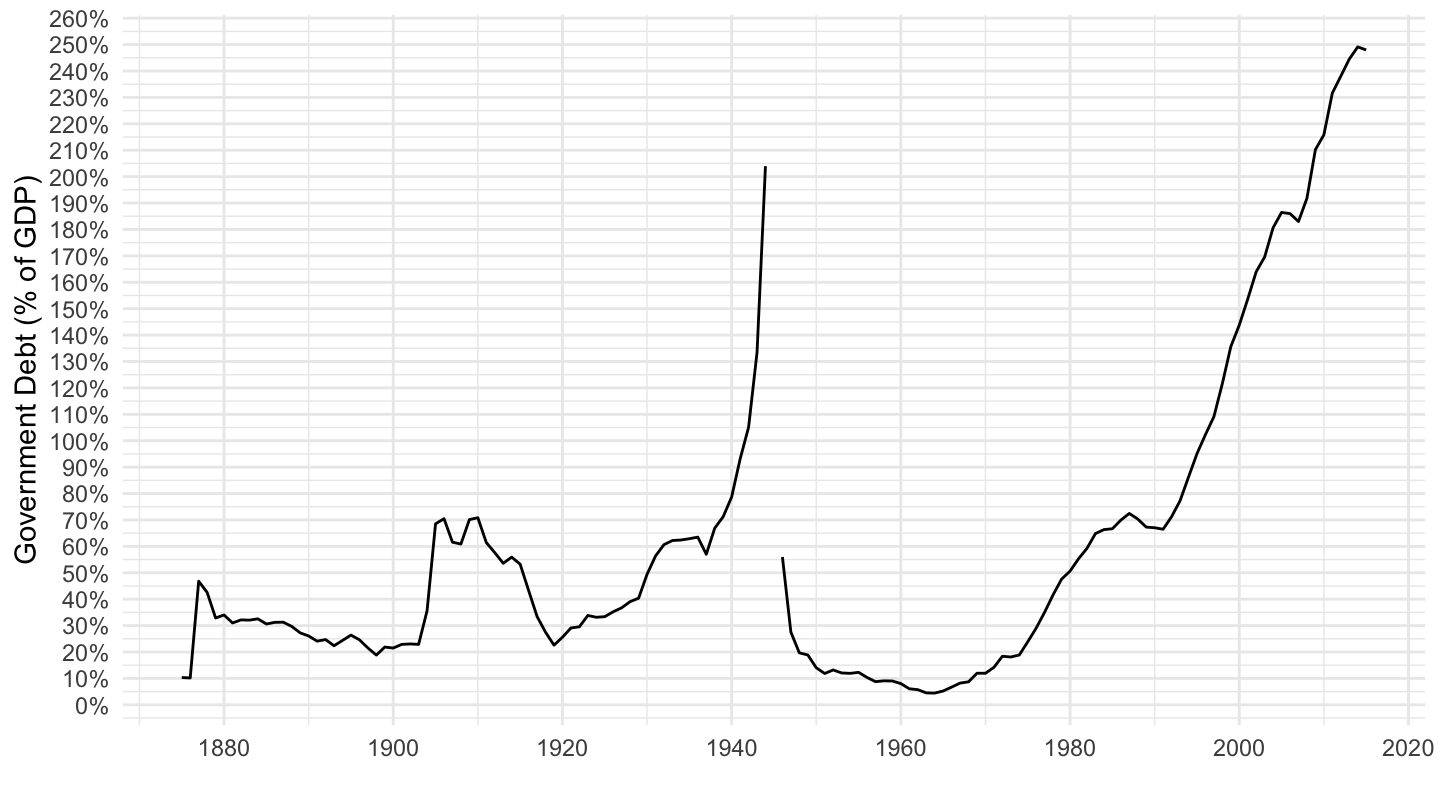
GGXWDG_GDP %>%
  year_to_date2() %>%
  filter(REF_AREA %in% c("DE")) %>%
  complete(date = seq.Date(min(date), max(date), by = "year")) %>%
  ggplot(.) + geom_line(aes(x = date, y = OBS_VALUE / 100)) + theme_minimal() +
  scale_y_continuous(breaks = 0.01*seq(0, 260, 10),
                     labels = scales::percent_format(accuracy = 1)) +
  scale_x_date(breaks = as.Date(paste0(seq(1700, 2100, 20), "-01-01")),
               labels = date_format("%Y")) +
  xlab("") + ylab("Government Debt (% of GDP)")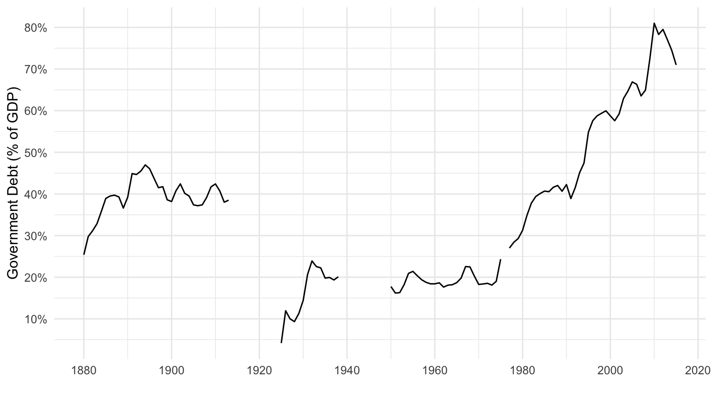
GGXWDG_GDP %>%
  year_to_date2() %>%
  filter(REF_AREA %in% c("IT")) %>%
  complete(date = seq.Date(min(date), max(date), by = "year")) %>%
  ggplot(.) + geom_line(aes(x = date, y = OBS_VALUE / 100)) + theme_minimal() +
  scale_y_continuous(breaks = 0.01*seq(0, 260, 10),
                     labels = scales::percent_format(accuracy = 1)) +
  scale_x_date(breaks = as.Date(paste0(seq(1700, 2100, 20), "-01-01")),
               labels = date_format("%Y")) +
  xlab("") + ylab("Government Debt (% of GDP)")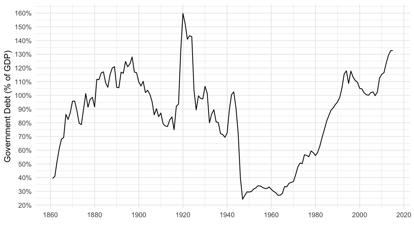
GGXWDG_GDP %>%
  year_to_date2() %>%
  filter(REF_AREA %in% c("DK")) %>%
  complete(date = seq.Date(min(date), max(date), by = "year")) %>%
  ggplot(.) + geom_line(aes(x = date, y = OBS_VALUE / 100)) + theme_minimal() +
  scale_y_continuous(breaks = 0.01*seq(0, 260, 10),
                     labels = scales::percent_format(accuracy = 1)) +
  scale_x_date(breaks = as.Date(paste0(seq(1700, 2100, 20), "-01-01")),
               labels = date_format("%Y")) +
  xlab("") + ylab("Government Debt (% of GDP)")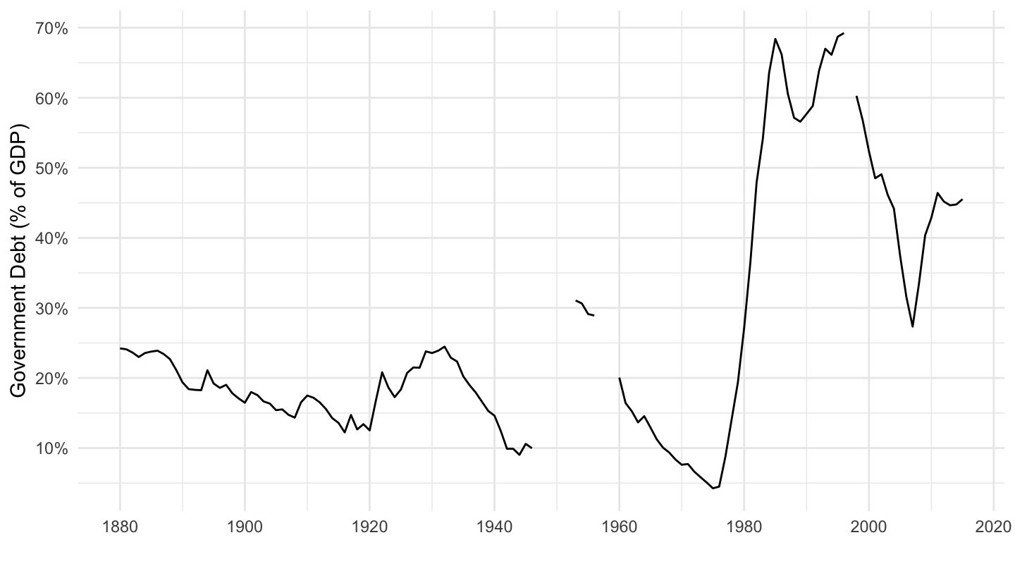
GGXWDG_GDP %>%
  year_to_date2() %>%
  filter(REF_AREA %in% c("DK"),
         date >= as.Date("1970-01-01"),
         date <= as.Date("2000-01-01")) %>%
  complete(date = seq.Date(min(date), max(date), by = "year")) %>%
  ggplot(.) + geom_line(aes(x = date, y = OBS_VALUE / 100)) + theme_minimal() +
  scale_y_continuous(breaks = 0.01*seq(0, 260, 10),
                     labels = scales::percent_format(accuracy = 1)) +
  scale_x_date(breaks = as.Date(paste0(seq(1700, 2100, 2), "-01-01")),
               labels = date_format("%Y")) +
  xlab("") + ylab("Government Debt (% of GDP)")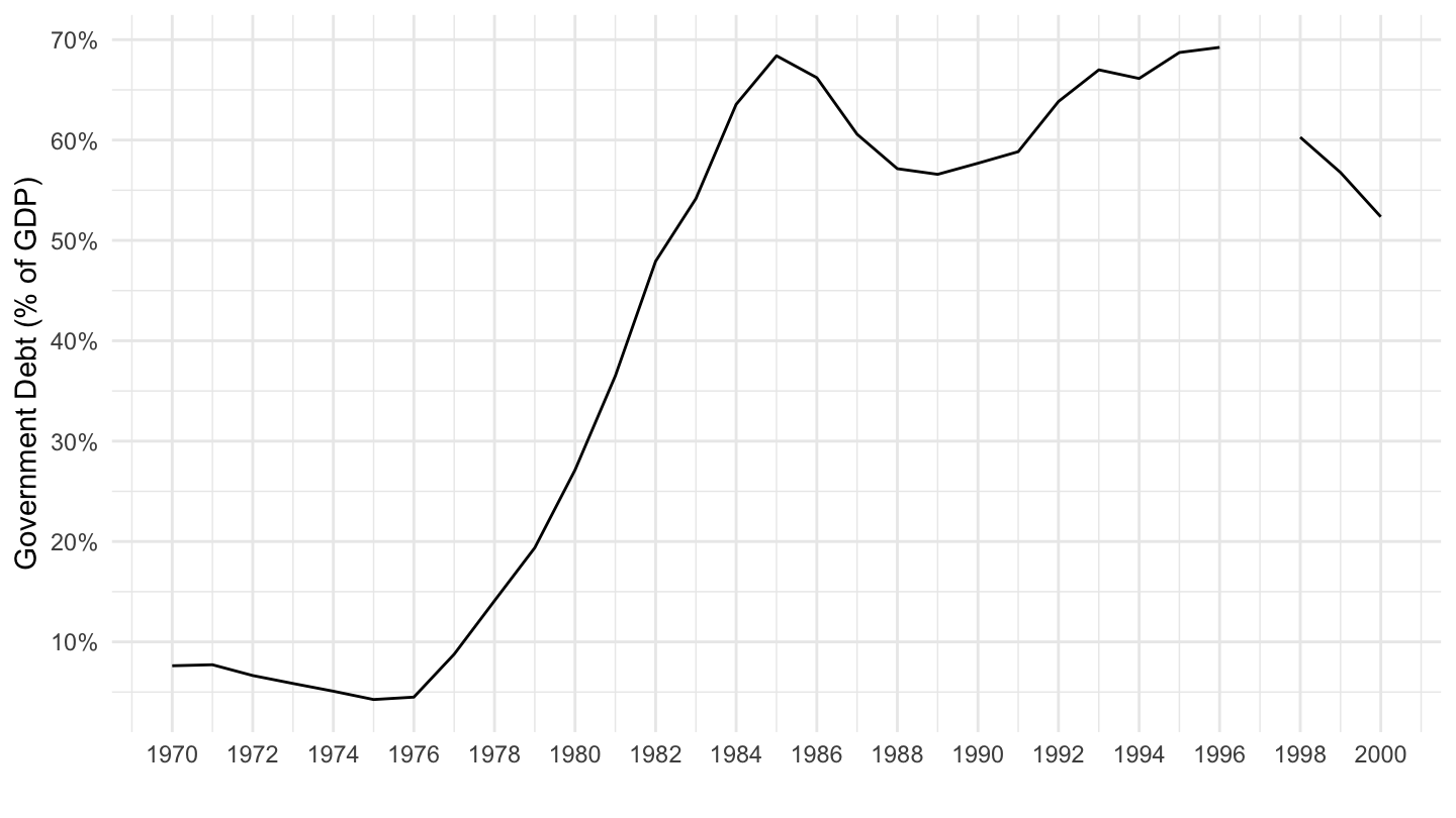
GGXWDG_GDP %>%
  year_to_date2() %>%
  filter(REF_AREA %in% c("ES")) %>%
  complete(date = seq.Date(min(date), max(date), by = "year")) %>%
  ggplot(.) + geom_line(aes(x = date, y = OBS_VALUE / 100)) + theme_minimal() +
  scale_y_continuous(breaks = 0.01*seq(0, 260, 10),
                     labels = scales::percent_format(accuracy = 1)) +
  scale_x_date(breaks = as.Date(paste0(seq(1700, 2100, 20), "-01-01")),
               labels = date_format("%Y")) +
  xlab("") + ylab("Government Debt (% of GDP)")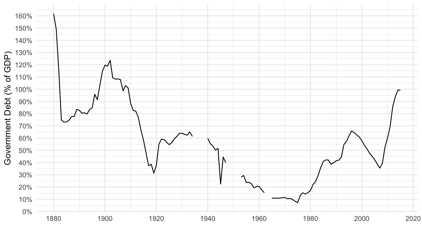
GGXWDG_GDP %>%
  filter(REF_AREA %in% c("BE")) %>%
  year_to_date2() %>%
  complete(date = seq.Date(min(date), max(date), by = "year")) %>%
  ggplot(.) + geom_line(aes(x = date, y = OBS_VALUE / 100)) + theme_minimal() +
  scale_y_continuous(breaks = 0.01*seq(0, 260, 10),
                     labels = scales::percent_format(accuracy = 1)) +
  scale_x_date(breaks = as.Date(paste0(seq(1700, 2100, 20), "-01-01")),
               labels = date_format("%Y")) +
  xlab("") + ylab("Government Debt (% of GDP)")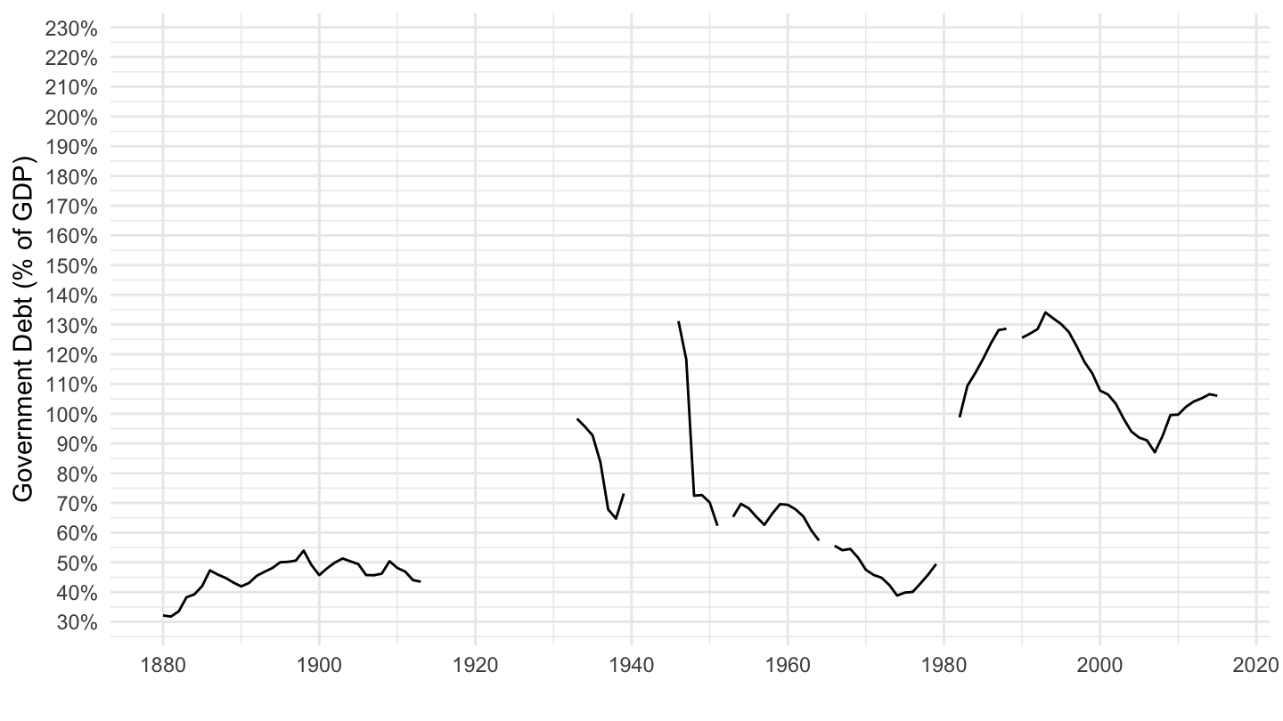
GGXWDG_GDP %>%
  filter(REF_AREA %in% c("CA")) %>%
  year_to_date2() %>%
  complete(date = seq.Date(min(date), max(date), by = "year")) %>%
  ggplot(.) + geom_line(aes(x = date, y = OBS_VALUE / 100)) + theme_minimal() +
  scale_y_continuous(breaks = 0.01*seq(0, 260, 10),
                     labels = scales::percent_format(accuracy = 1)) +
  scale_x_date(breaks = as.Date(paste0(seq(1700, 2100, 20), "-01-01")),
               labels = date_format("%Y")) +
  xlab("") + ylab("Government Debt (% of GDP)")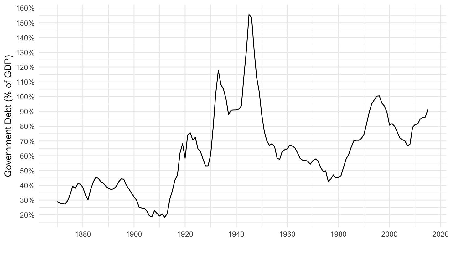
GGXWDG_GDP %>%
  filter(REF_AREA %in% c("GR")) %>%
  year_to_date2() %>%
  complete(date = seq.Date(min(date), max(date), by = "year")) %>%
  ggplot(.) + geom_line(aes(x = date, y = OBS_VALUE / 100)) + theme_minimal() +
  scale_y_continuous(breaks = 0.01*seq(0, 260, 10),
                     labels = scales::percent_format(accuracy = 1)) +
  scale_x_date(breaks = as.Date(paste0(seq(1700, 2100, 20), "-01-01")),
               labels = date_format("%Y")) +
  xlab("") + ylab("Government Debt (% of GDP)")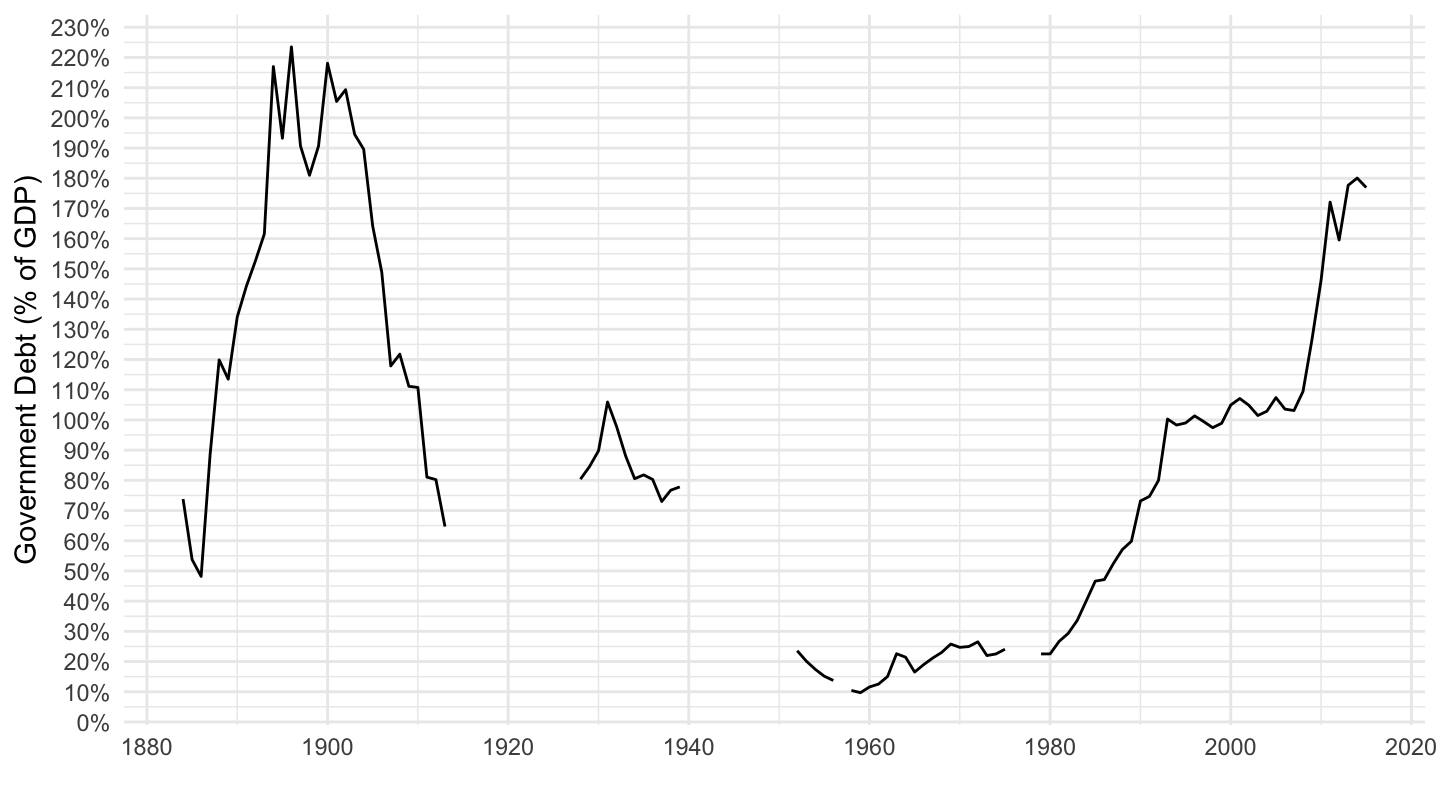
GGXWDG_GDP %>%
  filter(REF_AREA %in% c("PT")) %>%
  year_to_date2() %>%
  complete(date = seq.Date(min(date), max(date), by = "year")) %>%
  ggplot(.) + geom_line(aes(x = date, y = OBS_VALUE / 100)) + theme_minimal() +
  scale_y_continuous(breaks = 0.01*seq(0, 260, 10),
                     labels = scales::percent_format(accuracy = 1)) +
  scale_x_date(breaks = as.Date(paste0(seq(1700, 2100, 20), "-01-01")),
               labels = date_format("%Y")) +
  xlab("") + ylab("Government Debt (% of GDP)")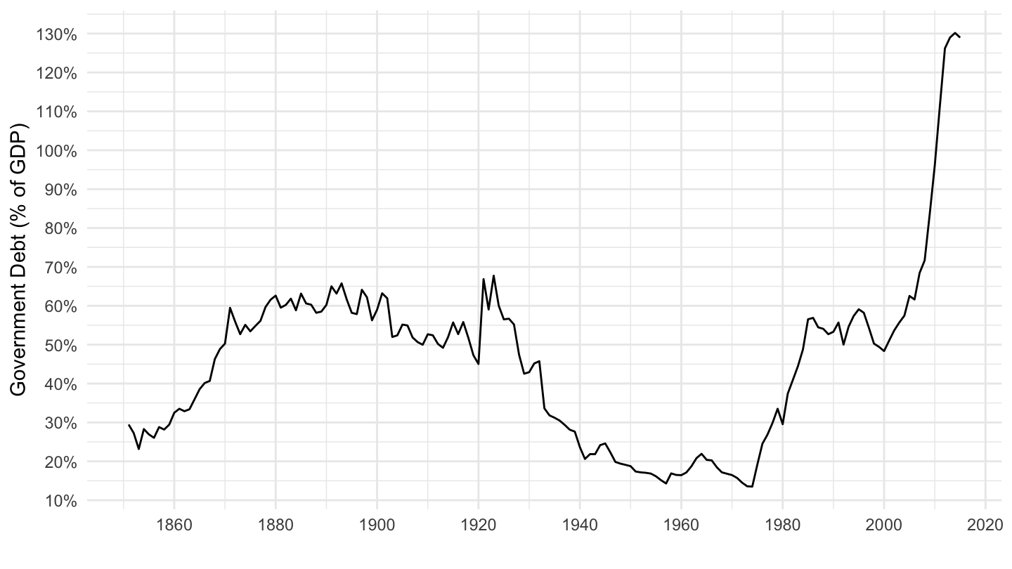
GGXWDG_GDP %>%
  filter(REF_AREA %in% c("LB")) %>%
  year_to_date2() %>%
  complete(date = seq.Date(min(date), max(date), by = "year")) %>%
  ggplot(.) + geom_line(aes(x = date, y = OBS_VALUE / 100)) + theme_minimal() +
  scale_y_continuous(breaks = 0.01*seq(0, 260, 10),
                     labels = scales::percent_format(accuracy = 1)) +
  scale_x_date(breaks = as.Date(paste0(seq(1700, 2100, 5), "-01-01")),
               labels = date_format("%Y")) +
  xlab("") + ylab("Government Debt (% of GDP)")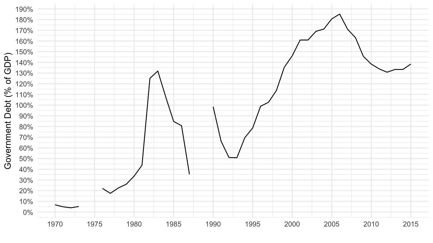
GGXWDG_GDP %>%
  filter(TIME_PERIOD == "2015") %>%
  arrange(-OBS_VALUE) %>%
  left_join(REF_AREA, by = "REF_AREA") %>%
  mutate(OBS_VALUE = round(OBS_VALUE) %>% paste0(., " %")) %>%
  select(REF_AREA, Ref_area, `Public Debt (2015)` = OBS_VALUE) %>%
  as.tibble %>%
  mutate(Flag = gsub(" ", "-", str_to_lower(gsub(" ", "-", Ref_area))),
         Flag = paste0('<img src="../../icon/flag/round/vsmall/', Flag, '.png" alt="Flag">')) %>%
  select(Flag, everything()) %>%
{if (is_html_output()) datatable(., filter = 'top', rownames = F, escape = F) else .}(ref:high-debt-to-gdp) Countries with debt > 90% of GDP.
GGXWDG_GDP %>%
  filter(TIME_PERIOD == "2015",
         OBS_VALUE > 90) %>%
  arrange(-OBS_VALUE) %>%
  left_join(REF_AREA, by = "REF_AREA") %>%
  mutate(OBS_VALUE = round(OBS_VALUE) %>% paste0(., " %")) %>%
  select(REF_AREA, Ref_area, `Public Debt (2015)` = OBS_VALUE) %>%
  as.tibble %>%
  mutate(Flag = gsub(" ", "-", str_to_lower(gsub(" ", "-", Ref_area))),
         Flag = paste0('<img src="../../icon/flag/round/vsmall/', Flag, '.png" alt="Flag">')) %>%
  select(Flag, everything()) %>%
{if (is_html_output()) datatable(., filter = 'top', rownames = F, escape = F) else .}GGXWDG_GDP %>%
filter(TIME_PERIOD == "2015",
OBS_VALUE < 20) %>%
arrange(-OBS_VALUE) %>%
left_join(REF_AREA, by = "REF_AREA") %>%
mutate(OBS_VALUE = round(OBS_VALUE) %>% paste0(., " %")) %>%
select(REF_AREA, Ref_area, `Public Debt (2015)` = OBS_VALUE) %>%
as.tibble %>%
mutate(Flag = gsub(" ", "-", str_to_lower(gsub(" ", "-", Ref_area))),
Flag = paste0('<img src="../../icon/flag/round/vsmall/', Flag, '.png" alt="Flag">')) %>%
select(Flag, everything()) %>%
{if (is_html_output()) datatable(., filter = 'top', rownames = F, escape = F) else .}GGXWDG_GDP %>%
filter(TIME_PERIOD == "2015") %>%
rename(iso2c = REF_AREA) %>%
right_join(world, by = "iso2c") %>%
ggplot() + theme_void() +
geom_polygon(aes(long, lat, group = group, fill = OBS_VALUE/100),
colour = alpha("black", 1/2), size = 0.1) +
scale_fill_viridis_c(name = "Debt to GDP (%)",
labels = scales::percent_format(accuracy = 1),
breaks = seq(0, 3, 0.4),
values = c(0, 0.2, 0.4, 0.6, 1)) +
theme(legend.position = c(0.1, 0.4),
legend.title = element_text(size = 10))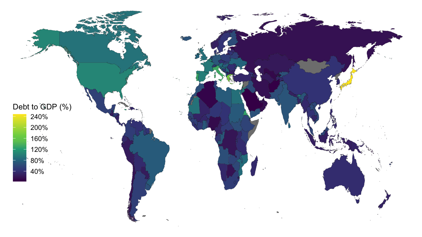
GGXWDG_GDP %>%
  filter(TIME_PERIOD == "2015") %>%
  rename(iso2c = REF_AREA) %>%
  right_join(europe, by = "iso2c") %>%
  ggplot() + theme_void() +
  geom_polygon(aes(long, lat, group = group, fill = OBS_VALUE/100),
               colour = alpha("black", 1/2), size = 0.1) +
  scale_fill_viridis_c(name = "Debt to GDP (%)",
                       labels = scales::percent_format(accuracy = 1),
                       breaks = seq(0, 3, 0.4),
                       values = c(0, 0.2, 0.4, 0.6, 1)) +
  theme(legend.position = c(0.1, 0.4),
        legend.title = element_text(size = 10))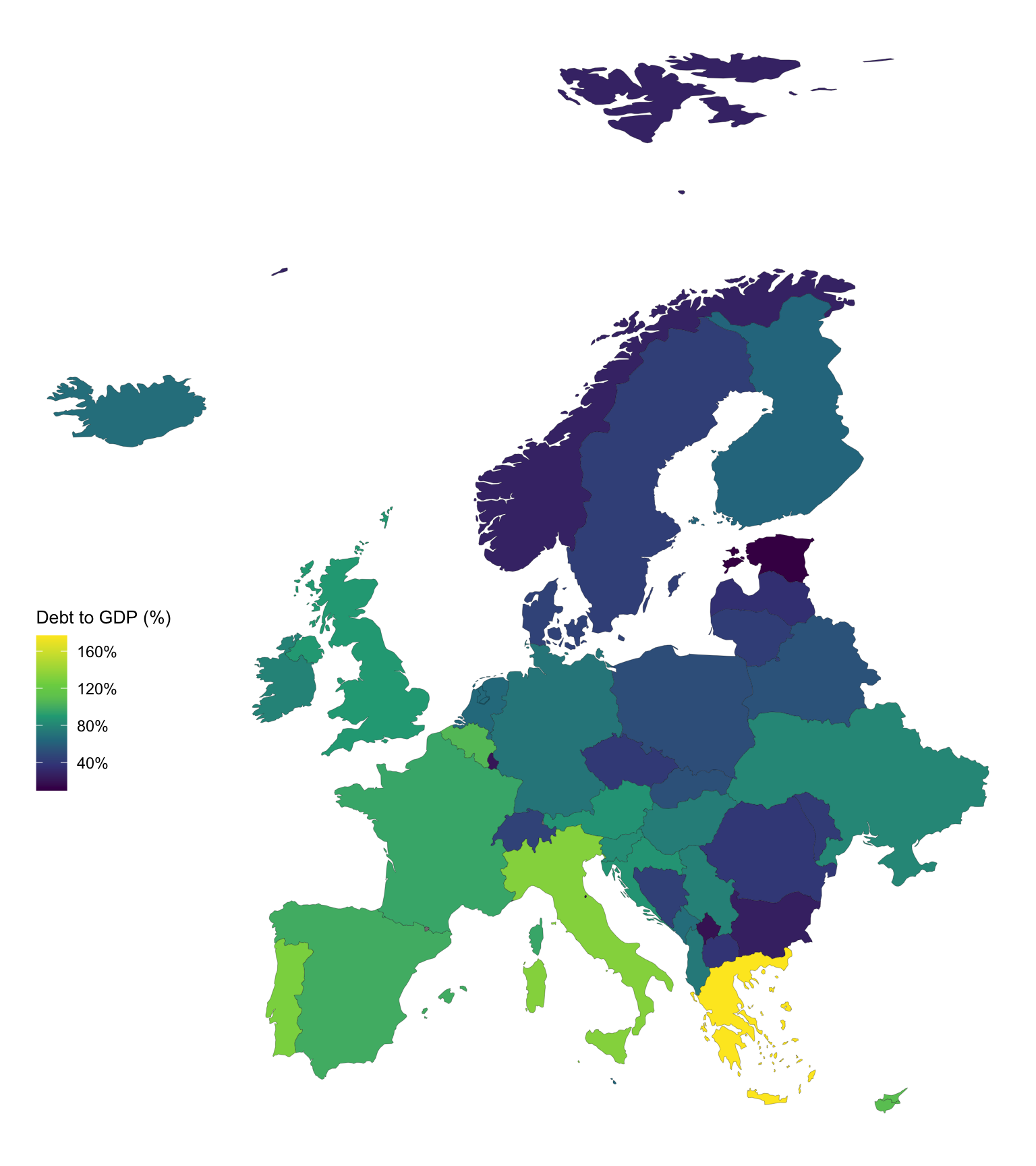
GGXWDG_GDP %>%
  filter(TIME_PERIOD == "2015") %>%
  rename(iso2c = REF_AREA) %>%
  right_join(eurozone_squeezed, by = "iso2c") %>%
  ggplot() + theme_void() +
  geom_polygon(aes(long, lat, group = group, fill = OBS_VALUE/100),
               colour = alpha("black", 1/2), size = 0.1) +
  scale_fill_viridis_c(name = "Debt to GDP (%)",
                       labels = scales::percent_format(accuracy = 1),
                       breaks = seq(0, 3, 0.4),
                       values = c(0, 0.2, 0.4, 0.6, 1)) +
  theme(legend.position = c(0.1, 0.9),
        legend.title = element_text(size = 10))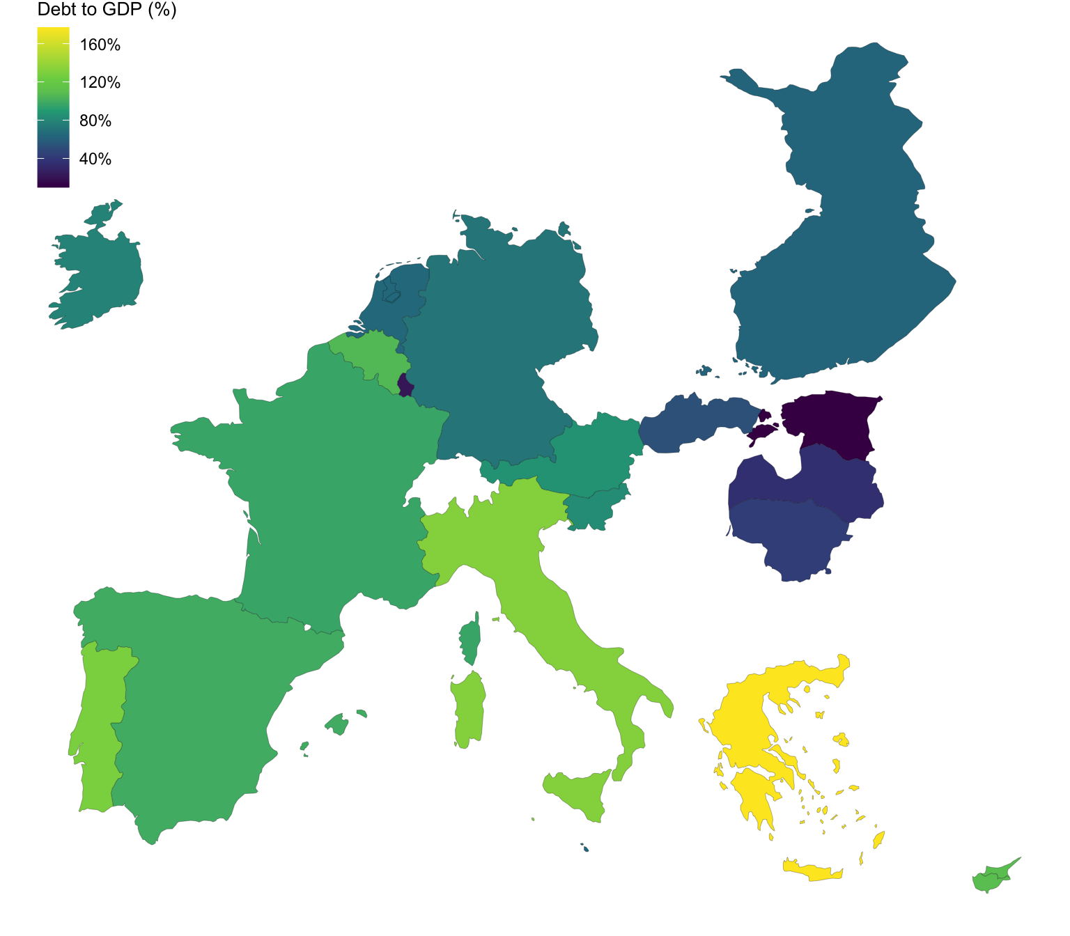
GGXWDG_GDP %>%
  year_to_date2() %>%
  filter(REF_AREA %in% c("FR", "IT", "JP"),
         date >= as.Date("1930-01-01"),
         date <= as.Date("1960-01-01")) %>%
  left_join(REF_AREA, by = "REF_AREA") %>%
  group_by(Ref_area) %>%
  complete(date = seq.Date(min(date), max(date), by = "year")) %>%
  ggplot(.) + theme_minimal() +
  geom_line(aes(x = date, y = OBS_VALUE / 100, color = Ref_area, linetype = Ref_area)) +
  scale_y_continuous(breaks = 0.01*seq(0, 260, 10),
                     labels = scales::percent_format(accuracy = 1)) +
  scale_color_manual(values = viridis(5)[1:4]) +
  theme(legend.position = c(0.75, 0.75),
        legend.title = element_blank()) +
  scale_x_date(breaks = as.Date(paste0(seq(1700, 2100, 5), "-01-01")),
               labels = date_format("%Y")) +
  xlab("") + ylab("Government Debt (% of GDP)")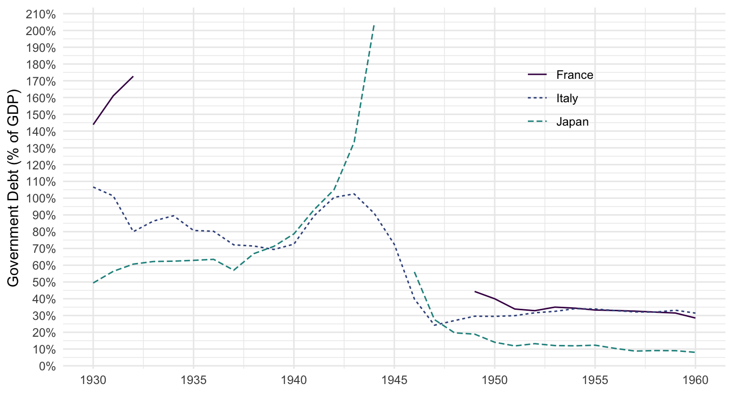
GGXWDG_GDP %>%
  year_to_date2() %>%
  filter(REF_AREA %in% c("DE", "US", "UK"),
         date >= as.Date("1930-01-01"),
         date <= as.Date("1960-01-01")) %>%
  left_join(REF_AREA, by = "REF_AREA") %>%
  group_by(Ref_area) %>%
  complete(date = seq.Date(min(date), max(date), by = "year")) %>%
  na.omit %>%
  ggplot(.) + theme_minimal() +
  geom_line(aes(x = date, y = OBS_VALUE / 100, color = Ref_area, linetype = Ref_area)) +
  scale_y_continuous(breaks = 0.01*seq(0, 300, 10),
                     labels = scales::percent_format(accuracy = 1)) +
  scale_color_manual(values = viridis(5)[1:4]) +
  theme(legend.position = c(0.85, 0.85),
        legend.title = element_blank()) +
  scale_x_date(breaks = as.Date(paste0(seq(1700, 2100, 5), "-01-01")),
               labels = date_format("%Y")) +
  xlab("") + ylab("Government Debt (% of GDP)")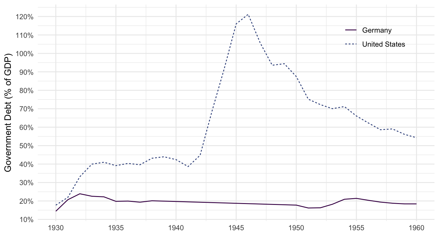
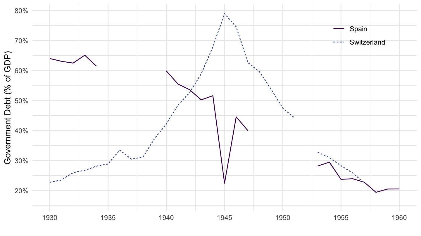
GGXWDG_GDP %>%
  year_to_date2() %>%
  filter(REF_AREA %in% c("ES", "CH"),
         date >= as.Date("1930-01-01"),
         date <= as.Date("1960-01-01")) %>%
  left_join(REF_AREA, by = "REF_AREA") %>%
  group_by(Ref_area) %>%
  complete(date = seq.Date(min(date), max(date), by = "year")) %>%
  ggplot(.) + theme_minimal() +
  geom_line(aes(x = date, y = OBS_VALUE / 100, color = Ref_area, linetype = Ref_area)) +
  scale_y_continuous(breaks = 0.01*seq(0, 300, 10),
                     labels = scales::percent_format(accuracy = 1)) +
  scale_color_manual(values = viridis(5)[1:4]) +
  theme(legend.position = c(0.85, 0.85),
        legend.title = element_blank()) +
  scale_x_date(breaks = as.Date(paste0(seq(1700, 2100, 5), "-01-01")),
               labels = date_format("%Y")) +
  xlab("") + ylab("Government Debt (% of GDP)")