Debt
Data
François Geerolf
Variables
Metadata
| Ticker | Name | Metadata |
|---|---|---|
| GVDPDEU | Germany Government Debt per GDP | NA |
| GVDPFRA | France Government Debt per GDP | NA |
| GVDPGBR | Great Britain Government Debt per GDP | NA |
| GVDPITA | Italy Government Debt per GDP | Notes: The method used is the model-based approach as given in the program TRAMO-SEATS. Working DAy adjustment is applied to the basic monthly indicators (where available) Seasonal adjustment is applied to the working day adjusted quarterly indicators. Data are disseminated in millions of euro on GDP at current and constant 1995 prices, together with implicit deflators, compiled using the expenditure approach and the production approach. The data cover the entire economy. Data are disseminated on current and constant price GDP showing a breakdown by expenditure category as follows: (1) compensation of employees (further broken down by productive sector); (2) gross fixed capital formation (further broken down by productive sector); (3) final domestic consumption (further broken down by purpose and by type of good); and (4) labor input (in full-time equivalents). The data are disseminated in both unadjusted and seasonally-adjusted formats. |
| GVDPJPN | Japan Government Debt per GDP | NA |
| GVDPPRT | Portugal General government gross debt, % of GDP | Source: Data from 1690 to 1989 are calculated by taking the amount of Government Central Debt and dividing it by the GDP of each country in local currency. Data from 1990 forward is taken from Kose, M. Ayhan, Sergio Kurlat, Franziska Ohnsorge, and Naotaka Sugawara (2017). “A Cross-Country Database of Fiscal Space.” World Bank Policy Research Working Paper 8157, World Bank, Washington, DC. Notes: Data from 1870 to 1970 are from Portuguese Historical Statistics, table 6.6C for 1870-1953 and table 6.6B for 1954-93 (http://www.ine.pt/xportal/xmain?xpid=INE&xpgid=ine_publicacoes&PUBLICACOESpub_boui=138364&PUBLICACOESmodo=2)Data are disseminated in millions of Euro on GDP in current prices and in constant 1995 prices, compiled by the expenditure and production methods. The data cover the entire economy of Portugal. The expenditure-based data are broken down into: private final consumption, collective consumption, gross fixed capital formation, imports of goods and services, and exports of goods and services. Private consumption (in the economic territory) is divided into: agriculture and food goods, durable goods, and current private consumption. Gross Capital Formation is divided into Gross Fixed Capital Formation, Acquisitions Less Disposable of Valuables and Changes in Stocks. Gross fixed capital formation is divided into: agriculture products, machinery and other equipment, transport material, construction, and other products. Data on gross value added in constant 1995 prices is disseminated for the following activities: agriculture, hunting, forestry and fishing; electricity, gas and water; industry; trade, restaurants and hotels; transports and communications; banking, insurance and renting activities; other services. The estimates for all activities, except agriculture, and all expenditure categories, except collective consumption, are based on primary quarterly data collected during the period, and are compiled using econometric techniques. The data for agriculture and collective consumption are based on primary annual data. The data are estimated according to the ESA (European System of Accounts) 95. The basic statistics are seasonally adjusted. |
France, Germany, U.K.
debt %>%
  left_join(iso3c, by = "iso3c") %>%
  filter(iso3c %in% c("DEU", "FRA", "GBR"),
         date >= as.Date("1925-01-01"),
         date <= as.Date("1970-01-01")) %>%
  group_by(iso3c_desc) %>%
  complete(date = seq.Date(min(date), max(date), by = "year")) %>%
  ggplot(.) +
  geom_line(aes(x = date, y = value/100, color = iso3c_desc, linetype = iso3c_desc)) +
  theme_minimal() + xlab("") + ylab("Government Debt (% of GDP)") +
  scale_y_continuous(breaks = 0.01*seq(0, 260, 20),
                     labels = scales::percent_format(accuracy = 1)) +
  scale_x_date(breaks = seq(1925, 2020, 5) %>% paste0("-01-01") %>% as.Date,
               labels = date_format("%y")) +
  scale_color_manual(values = viridis(5)[1:4]) +
  theme(legend.position = c(0.8, 0.8),
        legend.title = element_blank())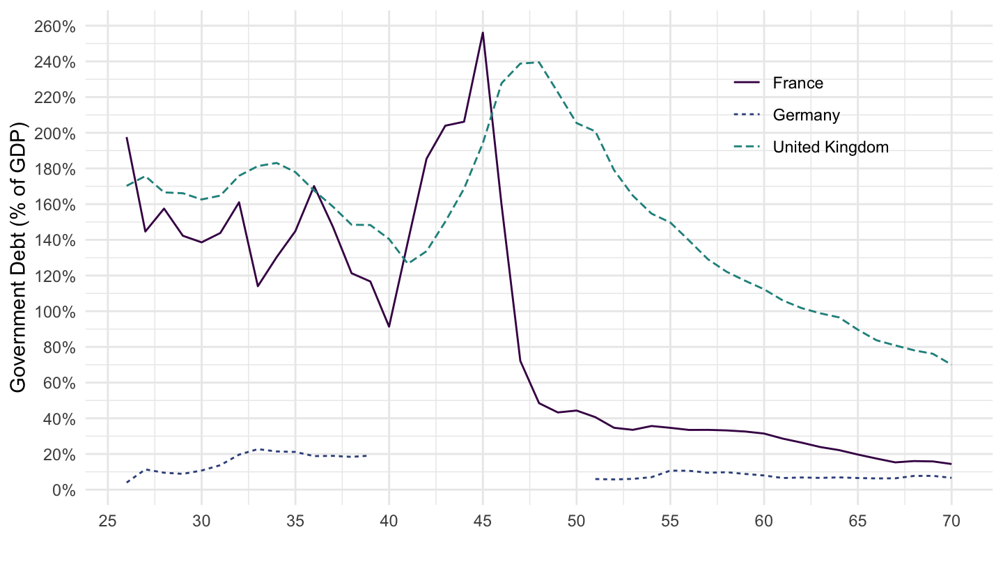
France
debt %>%
  filter(iso3c %in% c("FRA")) %>%
  select(date, value) %>%
  mutate(value = value / 100) %>%
  na.omit %>%
  ggplot(.) + geom_line(aes(x = date, y = value)) + theme_minimal() +
  scale_y_continuous(breaks = 0.01*seq(0, 260, 10),
                     labels = scales::percent_format(accuracy = 1)) +
  scale_x_date(breaks = as.Date(paste0(seq(1700, 2020, 20), "-01-01")),
               labels = date_format("%Y")) +
  xlab("") + ylab("France Government Debt (% of GDP)")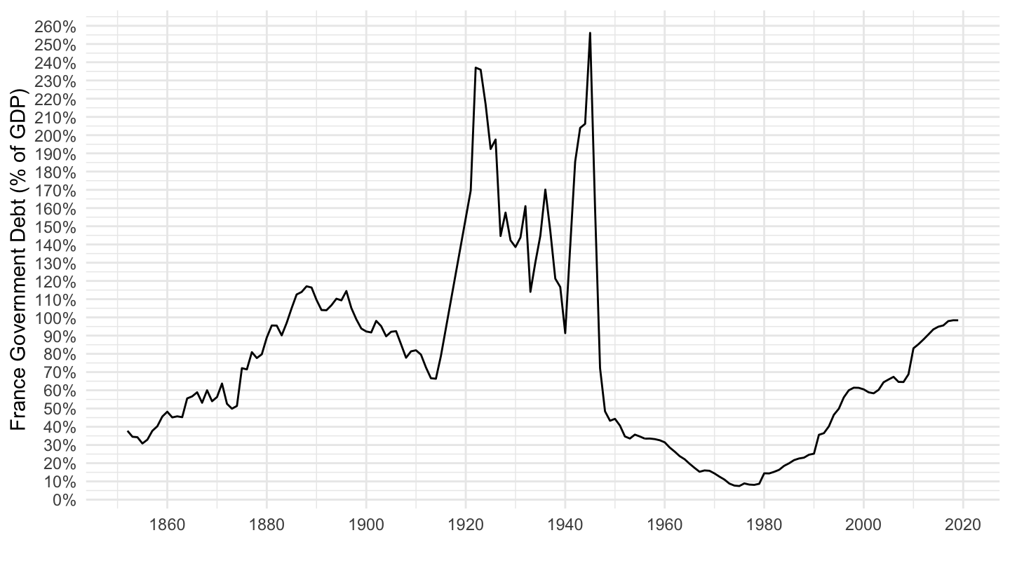
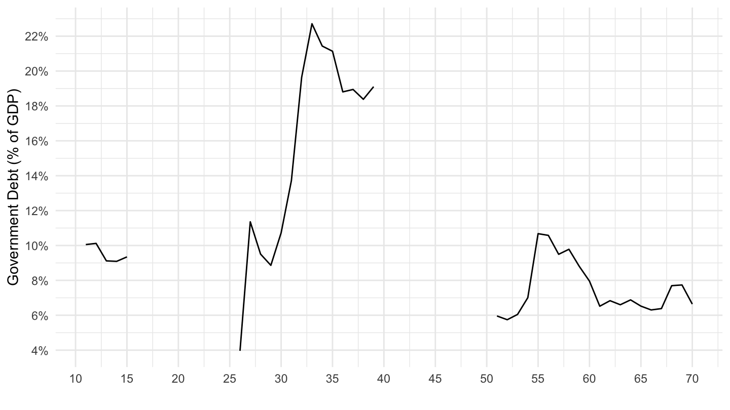
Germany
debt %>%
  filter(iso3c %in% c("DEU"),
         date >= as.Date("1910-01-01"),
         date <= as.Date("1970-01-01")) %>%
  complete(date = seq.Date(min(date), max(date), by = "year")) %>%
  ggplot(.) +
  geom_line(aes(x = date, y = value/100)) +
  theme_minimal() + xlab("") + ylab("Government Debt (% of GDP)") +
  scale_y_continuous(breaks = 0.01*seq(0, 260, 2),
                     labels = scales::percent_format(accuracy = 1)) +
  scale_x_date(breaks = seq(1800, 2020, 5) %>% paste0("-01-01") %>% as.Date,
               labels = date_format("%y")) +
  scale_color_manual(values = viridis(5)[1:4]) +
  theme(legend.position = c(0.8, 0.8),
        legend.title = element_blank())