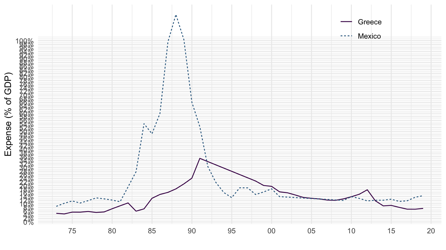
Last observation: 2024 (N = 105)
First observation: 1972 (N = 35)
Last data update: 07 oct. 2026, 00:48
Last compile: 07 oct. 2026, 00:56
GC.XPN.INTP.RV.ZS |>
  left_join(iso2c, by = "iso2c") |>
  group_by(iso2c, Iso2c) |>
  mutate(value = round(value, 2)) |>
  summarise(Nobs = n(),
            `Year 1` = first(year),
            `HH Consumption 1 (%)` = first(value),
            `Year 2` = last(year),
            `HH Consumption 2 (%)` = last(value)) |>
  arrange(-Nobs) %>%
{if (is_html_output()) datatable(., filter = 'top', rownames = F) else .}GC.XPN.INTP.RV.ZS |>
filter(iso2c %in% c("IT", "FR", "DE")) |>
left_join(iso2c, by = "iso2c") |>
year_to_enddate() |>
mutate(value = value/100) |>
add_flag_color("Iso2c") |>
ggplot() + theme_minimal() + geom_line() +
aes(x = date, y = value, color = color) +
xlab("") + ylab("Expense (% of GDP)") +
scale_color_identity() + add_flags +
theme(legend.title = element_blank(),
legend.position = c(0.1, 0.9)) +
scale_x_date(breaks = seq(1950, 2100, 5) |> paste0("-01-01") |> as.Date(),
labels = date_format("%Y")) +
scale_y_continuous(breaks = 0.01*seq(-60, 100, 2),
labels = scales::percent_format(accuracy = 1))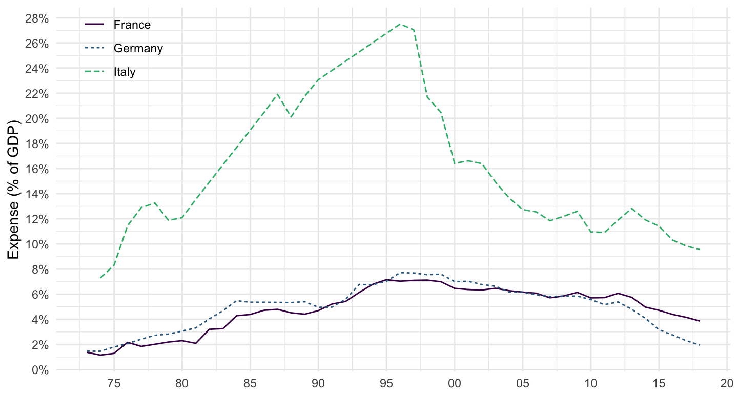
GC.XPN.INTP.RV.ZS |>
  filter(iso2c %in% c("JP", "CH")) |>
  left_join(iso2c, by = "iso2c") |>
  year_to_enddate() |>
  mutate(value = value/100) |>
  add_flag_color("Iso2c") |>
  ggplot() + theme_minimal() + geom_line() +
  aes(x = date, y = value, color = color) +
  xlab("") + ylab("Expense (% of GDP)") +
  scale_color_identity() + add_flags +
  theme(legend.title = element_blank(),
        legend.position = c(0.8, 0.9)) +
  scale_x_date(breaks = seq(1950, 2100, 5) |> paste0("-01-01") |> as.Date(),
               labels = date_format("%Y")) +
  scale_y_continuous(breaks = 0.01*seq(-60, 60, 2),
                     labels = scales::percent_format(accuracy = 1))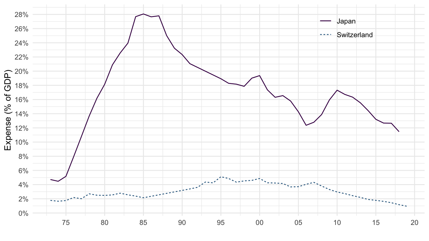
GC.XPN.INTP.RV.ZS |>
  filter(iso2c %in% c("CN", "US")) |>
  left_join(iso2c, by = "iso2c") |>
  year_to_enddate() |>
  mutate(value = value/100) |>
  add_flag_color("Iso2c") |>
  ggplot() + theme_minimal() + geom_line() +
  aes(x = date, y = value, color = color) +
  xlab("") + ylab("Expense (% of GDP)") +
  scale_color_identity() + add_flags +
  theme(legend.title = element_blank(),
        legend.position = c(0.2, 0.9)) +
  scale_x_date(breaks = seq(1950, 2100, 5) |> paste0("-01-01") |> as.Date(),
               labels = date_format("%Y")) +
  scale_y_continuous(breaks = 0.01*seq(-60, 100, 2),
                     labels = scales::percent_format(accuracy = 1))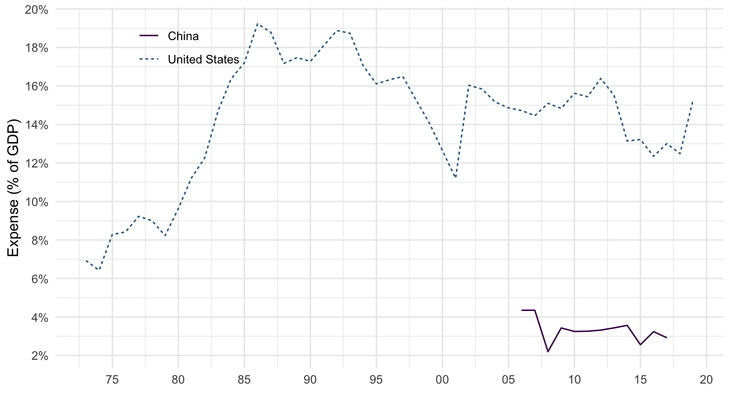
GC.XPN.INTP.RV.ZS |>
  filter(iso2c %in% c("CN", "FR", "DE")) |>
  left_join(iso2c, by = "iso2c") |>
  year_to_enddate() |>
  mutate(value = value/100) |>
  add_flag_color("Iso2c") |>
  ggplot() + theme_minimal() + geom_line() +
  aes(x = date, y = value, color = color) +
  xlab("") + ylab("Expense (% of GDP)") +
  scale_color_identity() + add_flags +
  theme(legend.title = element_blank(),
        legend.position = c(0.15, 0.9)) +
  scale_x_date(breaks = seq(1950, 2100, 5) |> paste0("-01-01") |> as.Date(),
               labels = date_format("%Y")) +
  scale_y_continuous(breaks = 0.01*seq(-60, 100, 2),
                     labels = scales::percent_format(accuracy = 1))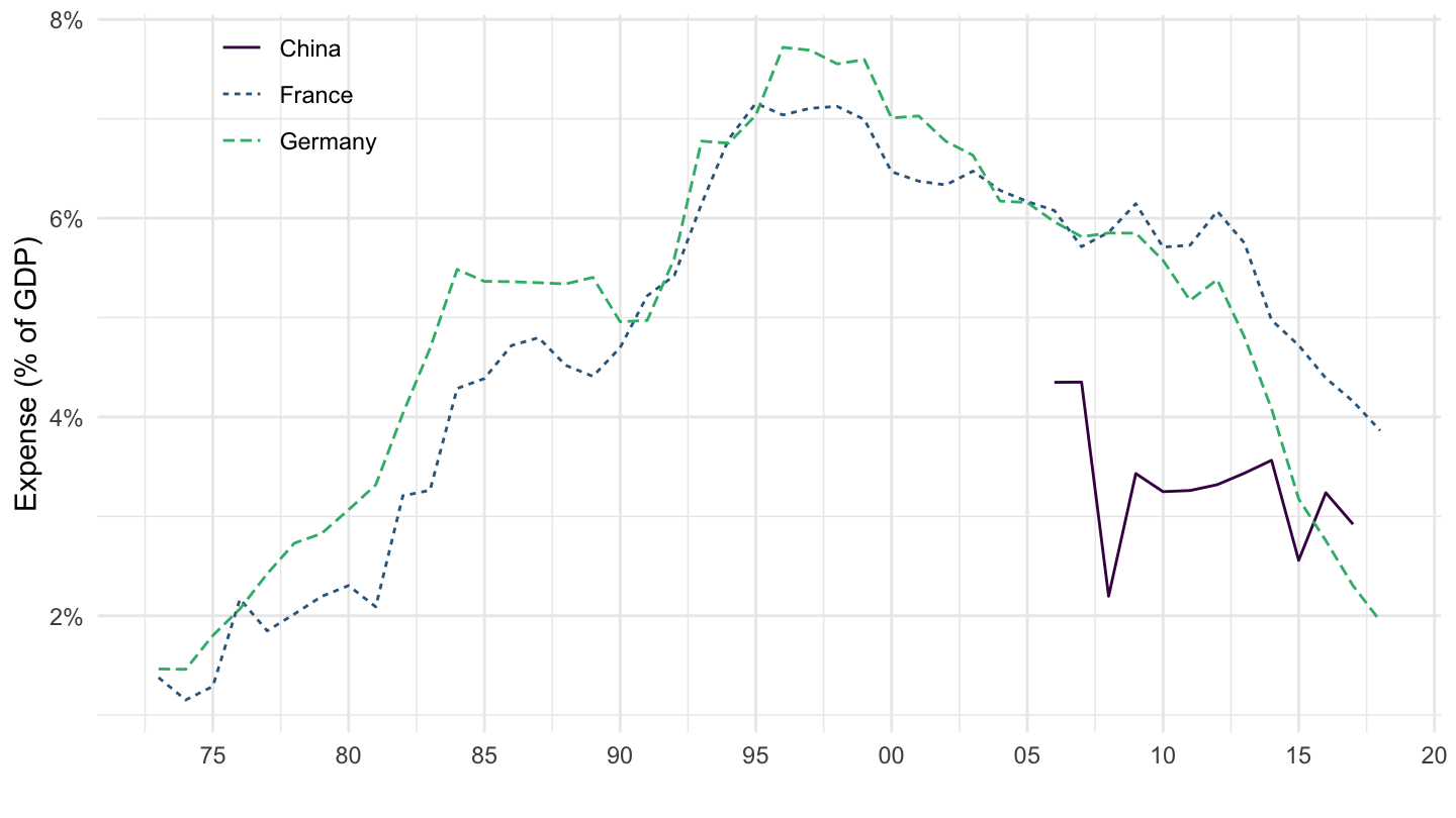
GC.XPN.INTP.RV.ZS |>
  filter(iso2c %in% c("US", "GB", "ES")) |>
  left_join(iso2c, by = "iso2c") |>
  year_to_enddate() |>
  mutate(value = value/100) |>
  add_flag_color("Iso2c") |>
  ggplot() + theme_minimal() + geom_line() +
  aes(x = date, y = value, color = color) +
  xlab("") + ylab("Expense (% of GDP)") +
  scale_color_identity() + add_flags +
  theme(legend.title = element_blank(),
        legend.position = c(0.4, 0.9)) +
  scale_x_date(breaks = seq(1950, 2100, 5) |> paste0("-01-01") |> as.Date(),
               labels = date_format("%Y")) +
  scale_y_continuous(breaks = 0.01*seq(-60, 100, 2),
                     labels = scales::percent_format(accuracy = 1))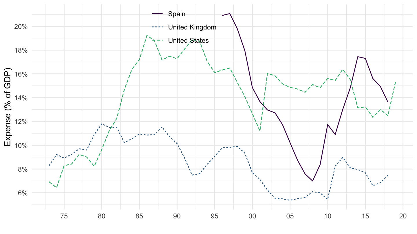
GC.XPN.INTP.RV.ZS |>
  filter(iso2c %in% c("AR", "CL", "VE")) |>
  left_join(iso2c, by = "iso2c") |>
  year_to_enddate() |>
  mutate(Iso2c = ifelse(iso2c == "VE", "Venezuela", Iso2c)) |>
  mutate(value = value/100) |>
  add_flag_color("Iso2c") |>
  ggplot() + theme_minimal() + geom_line() +
  aes(x = date, y = value, color = color) +
  xlab("") + ylab("Expense (% of GDP)") +
  scale_color_identity() + add_flags +
  theme(legend.title = element_blank(),
        legend.position = c(0.8, 0.9)) +
  scale_x_date(breaks = seq(1950, 2100, 5) |> paste0("-01-01") |> as.Date(),
               labels = date_format("%Y")) +
  scale_y_continuous(breaks = 0.01*seq(-60, 100, 2),
                     labels = scales::percent_format(accuracy = 1))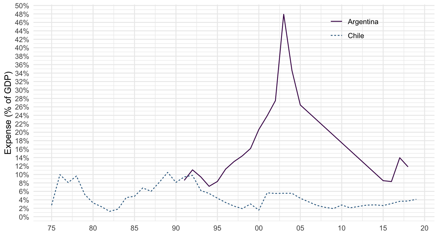
GC.XPN.INTP.RV.ZS |>
  filter(iso2c %in% c("GR", "HK", "MX")) |>
  left_join(iso2c, by = "iso2c") |>
  year_to_enddate() |>
  mutate(Iso2c = ifelse(iso2c == "HK", "Hong Kong", Iso2c)) |>
  mutate(value = value/100) |>
  add_flag_color("Iso2c") |>
  ggplot() + theme_minimal() + geom_line() +
  aes(x = date, y = value, color = color) +
  xlab("") + ylab("Expense (% of GDP)") +
  scale_color_identity() + add_flags +
  theme(legend.title = element_blank(),
        legend.position = c(0.8, 0.9)) +
  scale_x_date(breaks = seq(1950, 2100, 5) |> paste0("-01-01") |> as.Date(),
               labels = date_format("%Y")) +
  scale_y_continuous(breaks = 0.01*seq(-60, 100, 2),
                     labels = scales::percent_format(accuracy = 1))