October 19, 2020
Keynesian Economics
Introduction
Opens a set of lectures on Keynesian economics.
Neoclassical models of consumption, saving, investment, labor market \(=\) mainstream paradigm in J.M. Keynes’ time.
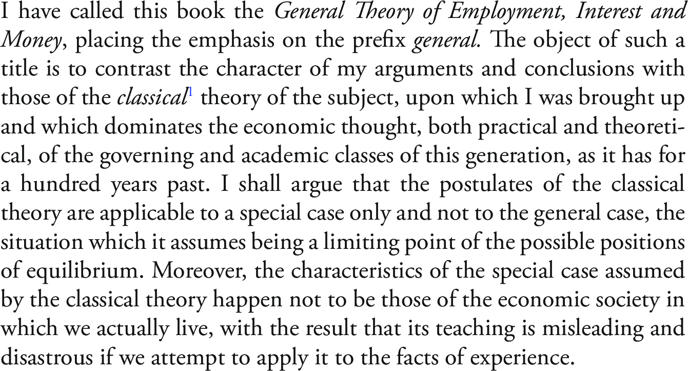
J.M. Keynes (1936) refers to this paradigm as “classical.”
Teaching of classical economics is “misleading and disastrous if we attempt to apply it to the facts of experience.”
First words of the General Theory - Keynes (1936)
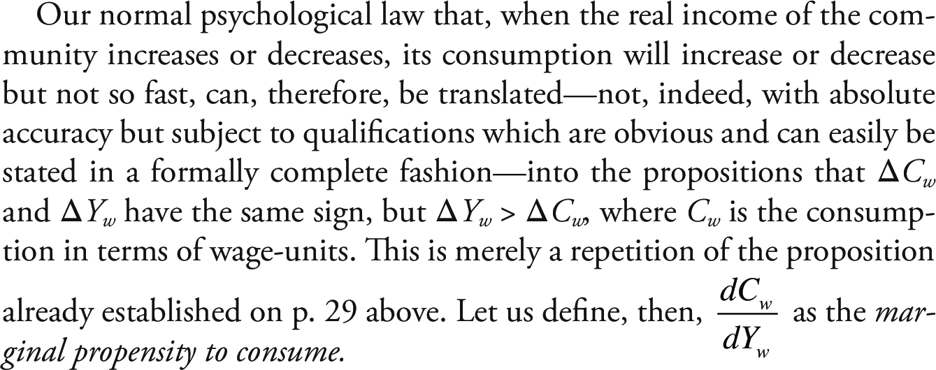
Marginal Propensity to Consume - Keynes (1936)
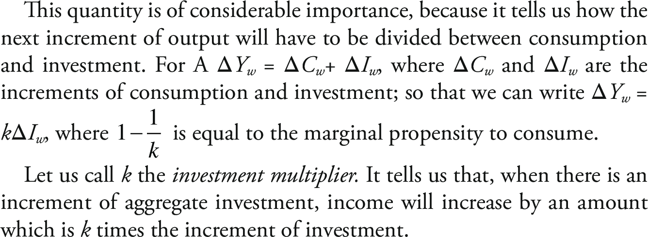
Multiplier (change in investment)
On Keynes
On J.M. Keynes - Joan Robinson (1974)
In 1931, when the world crisis had produced a sharp increase in the deficit on the U.K. balance of payments, the appropriate remedy (approved as much by the unlucky Labour government as by the Bank of England) was to cut expenditure so as to balance the budget. These were the orthodox views that prevailed in the realm of public policy.
In those years British orthodoxy was still dominated by nostalgia for the world before 1914. Then there was normality and equilibrium. To get back to that happy state, its institutions and its policies should be restored - keep to the gold standard at the old sterling parity, balance the budget, maintain free trade and observe the strictest laissez faire in the relations of government with industry. When Lloyd George proposed a campaign to reduce unemployment (which was then at the figure of one million or more) by expenditure on public works, he was answered by the famous “Treasury View” that there is a certain amount of saving at any moment, available to finance investment, and if the government borrows a part, there will be so much the less for industry.
On J.M. Keynes - Joan Robinson (1974)
Meanwhile the Nazis had been proving Lloyd George’s point with a vengeance. It was a joke in Germany that Hitler was planning to give employment in straightening the Crooked Lake, painting the Black Forest white and putting down linoleum in the Polish Corridor. The Treasury view was that his unsound policies would soon bring him down. But the little group of Keynesians was despondent and frustrated. We were getting the theory clear at last, but it was going to be too late.
Similarly today, the rethinking in economic thought is in great part driven by politics.
Do politics “trump” economics?
Interest-inelastic investment
Strong Assumption
In the following notes, I assume that investment is interest inelastic.
In other words, it is assumed that investment does not much depend on the cost of capital.
In many textbooks, even Keynesian models feature a strong dependancy of investment on the cost of capital \(I(r)\): this is in fact what lies behind the (IS) curve.
Only assuming a “zero-lower bound,” or the fact that interest rates can’t fall below a certain threshold, do we have a “paradox of thrift.”
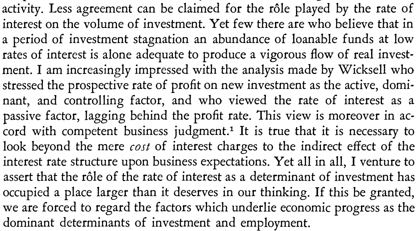
Hansen (1939)
To go further
In one of the last lectures of the course on theoretical controversies, we shall see that one reason why investment is not responsive to interest rates when they become low, is that “rational bubbles” can appear.
In other words, with low interest rates, more saving does not necessarily translate into more investment, but might alternatively translate into higher asset prices instead.
This is very different from the neoclassical, Solow growth model we saw before, in which capital accumulation depends a lot on the cost of capital.
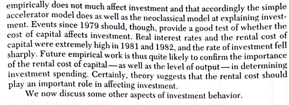
Empirically, it has been shown repeatedly that investment bears very little connection to the cost of capital. Thus, it is probably not such a strong assumption after all.
Dornbusch, Fischer (1979)
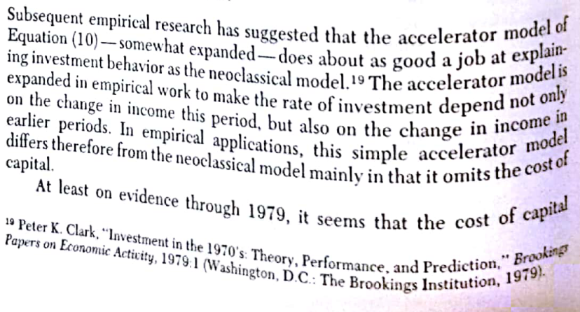
Dornbusch, Fischer (1979)
Keynesian Crosses
Goods Market Model (\(b_1=0\))
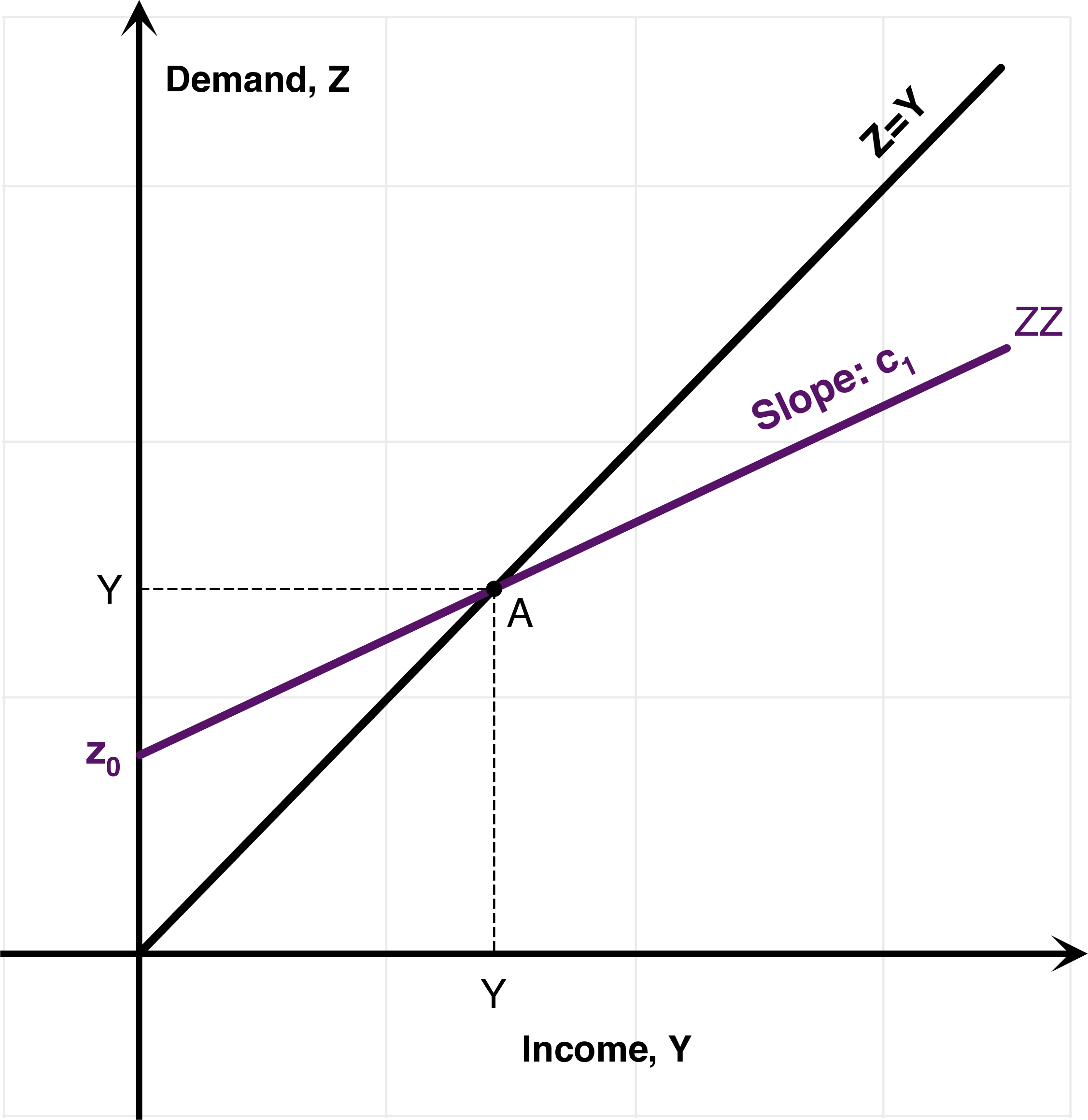
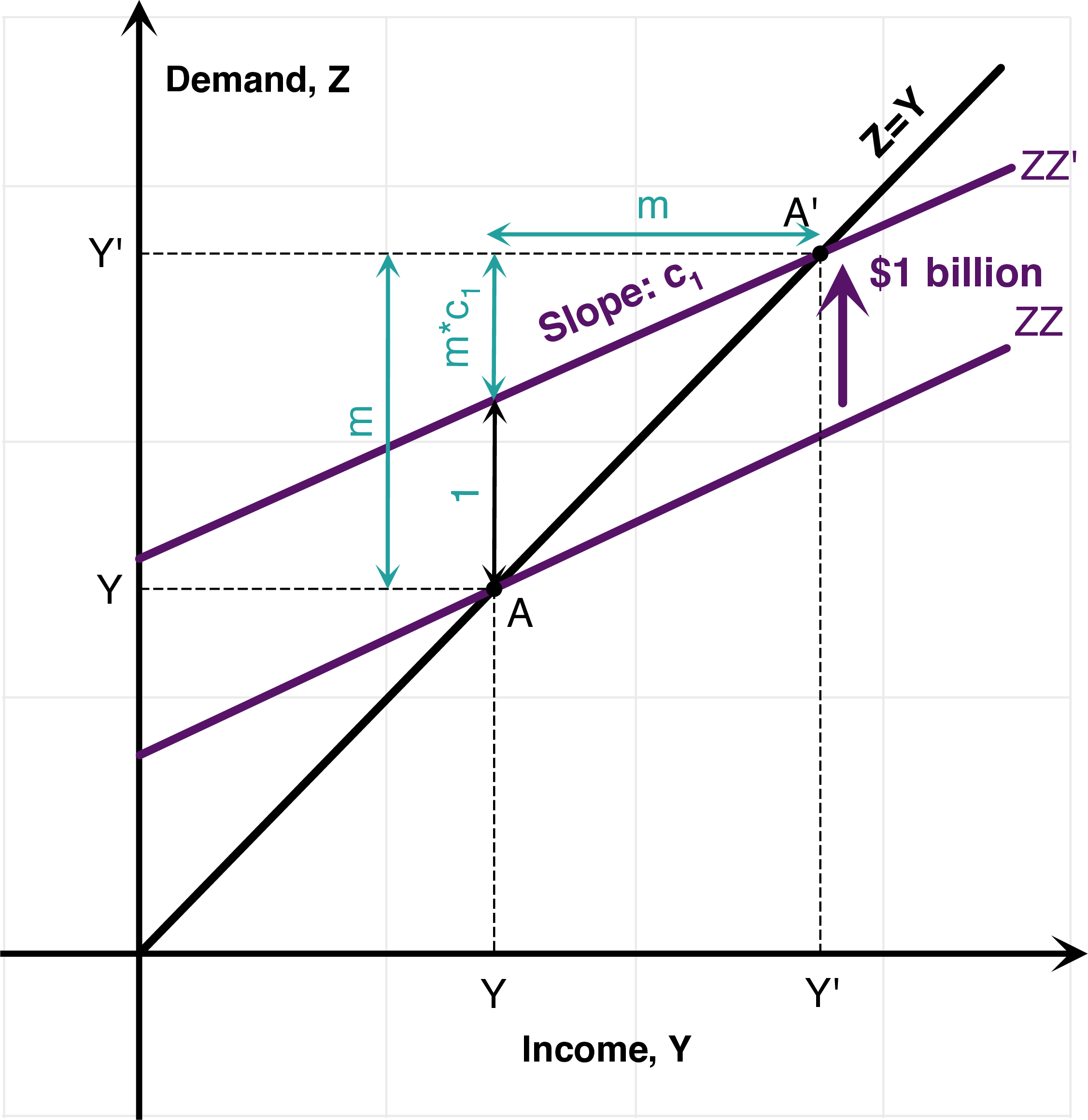
Keynesian Cross: Graphical Interpretation 1 (\(b_1=0\))
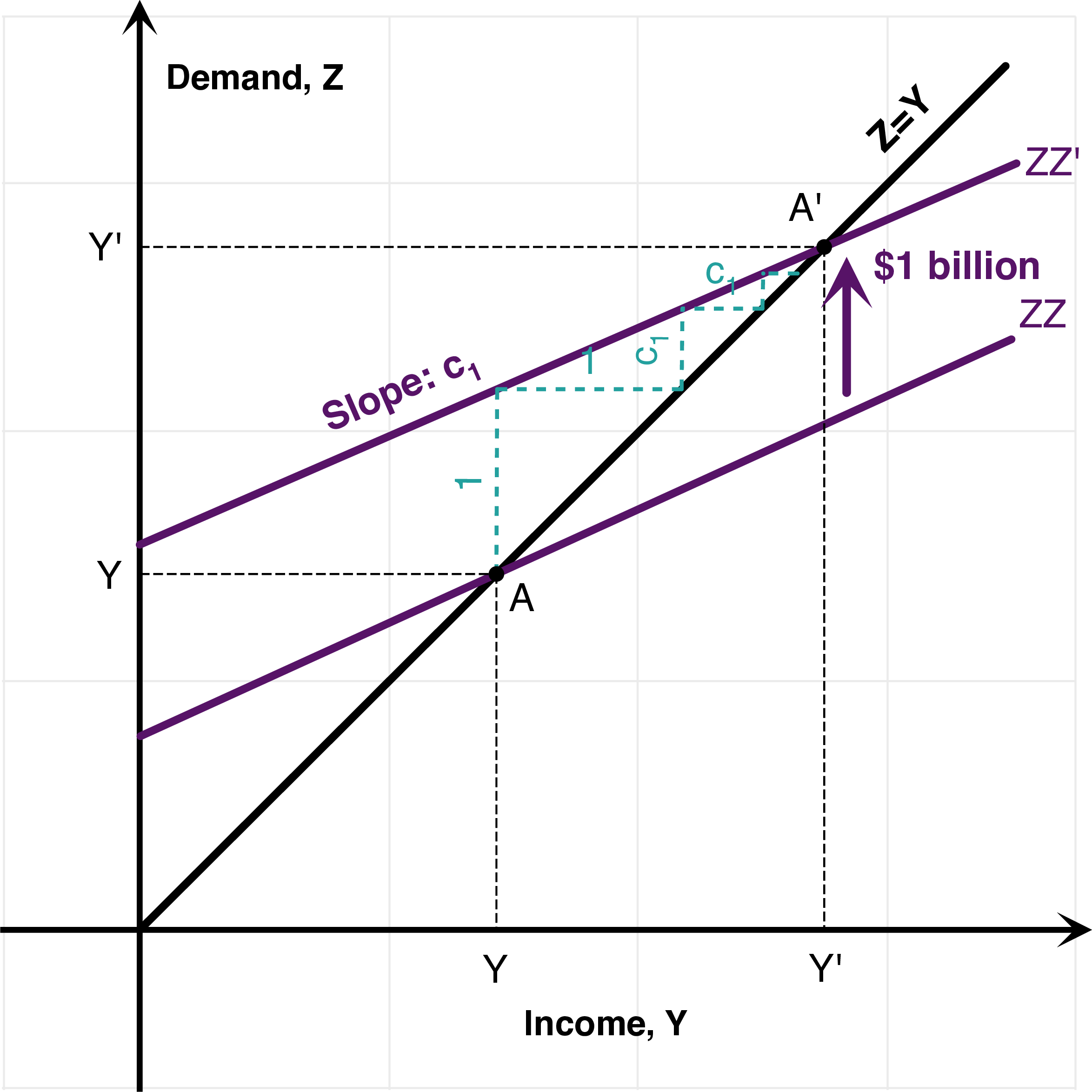
Keynesian Cross: Graphical Interpretation 2 (\(b_1=0\))
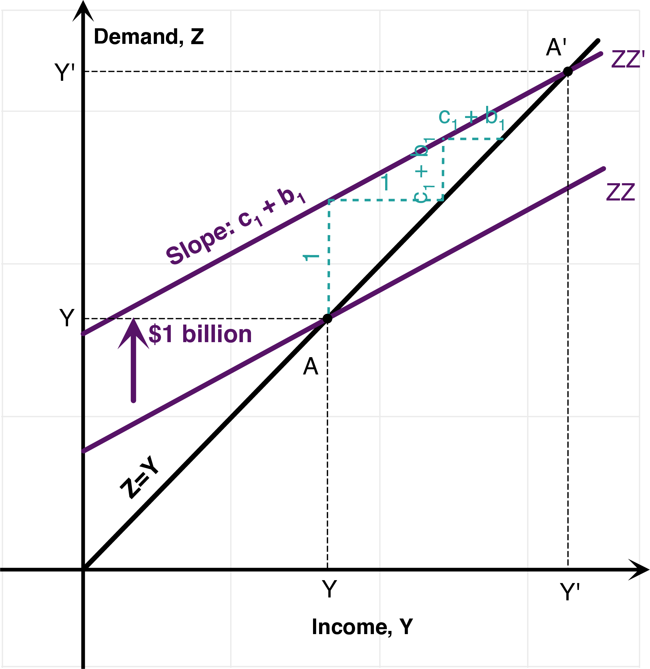
Accelerator Effect of Investment (\(b_1 \neq 0\))
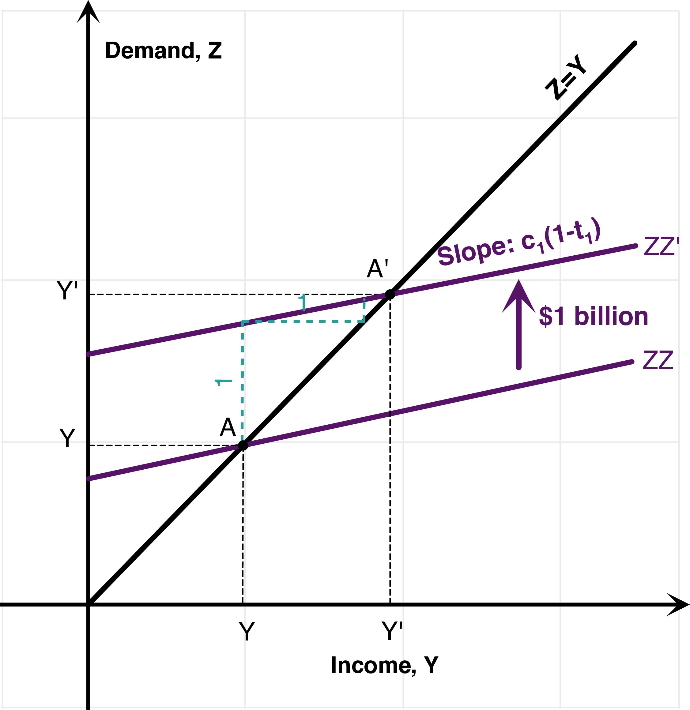
Automatic Stabilizers
Readings
Robert J. Barro - Keynes Is Still Dead.
This article from Robert Barro dates from just before the 1992 presidential election. (Clinton was president 1993-2001)
At the time, Keynesian economics was in decline. (the 2007-2009 financial crisis sparked a renewed interest in Keynesian economics)
Importantly, policy-making institutions (IMF, Treasuries) have always been more inclined towards Keynesian economics, while academics, at least until recently, have taken a more skeptical approach.
Robert Barro pushed the idea of “Ricardian equivalence”: the idea that Keynesian stimulus such as tax cuts, are ineffective because people anticipate future taxes to come, to repay the public debt.
Barro has used it to explain the absence of the crowding-out effects of government debt, particularly following the Reagan tax cuts. Of course, as we saw, an alternative explanation is that investment is not sensitive to the cost of capital, and mainly determined by aggregate demand.
Empirical Macro: Aggregate Studies
The Problem with Empirical Macro 1/3


The Problem with Empirical Macro 2/3
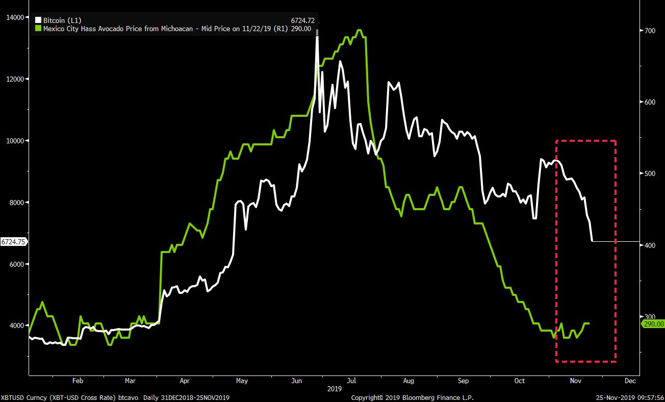
The Problem with Empirical Macro 3/3
Messerli (2012): Nobel Laureates and Chocolate Consumption.
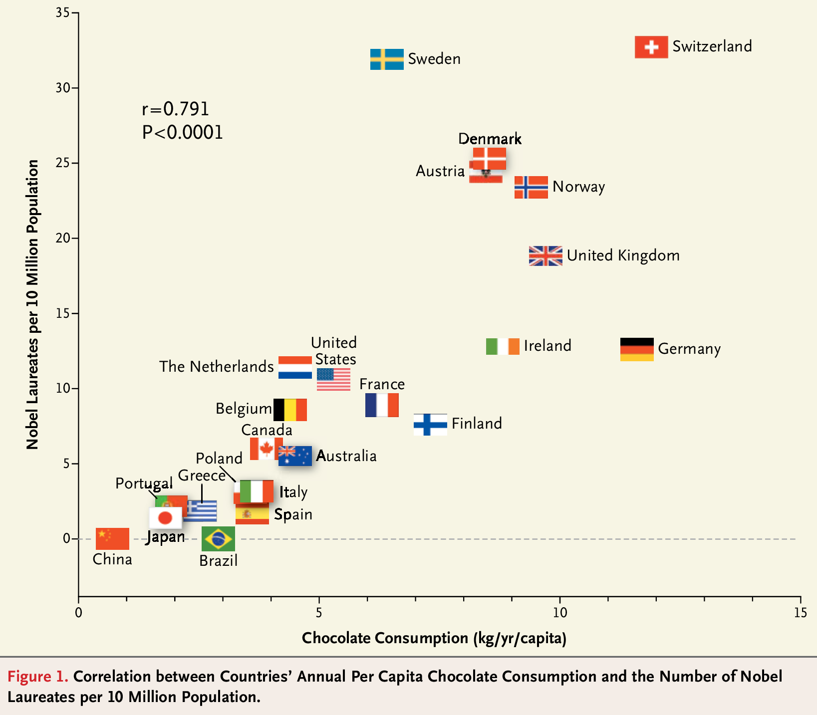
The Problem with Empirical Macro
Why don’t we just look at what happens to GDP following a tax cut?
Many things happen in any one year:
– September 15, 2013: Britney Spears happens to release her new song, which promotes work ethic.
– However, other things have happened between 2013 and 2018 (including a massive tax cut plan)Policies are changed for a reason:
– Years where taxes are changed are different from taxes where taxes are not changed.
– This is not like a Randomized Control Trial (RCT) in medicine: macroeconomic policies are not changed randomly.
– For example: \(\Delta G>0\) often happens during recessions. Low subsequent GDP growth: low multipliers or because GDP growth was low to start with.
Answers
What are the potential answers?
Add up many tax changes:
Some tax changes are accompanied by a new release of Britney Spears, but on average they are not.
Allows to control for other types of more serious events, too. (wars, etc.)
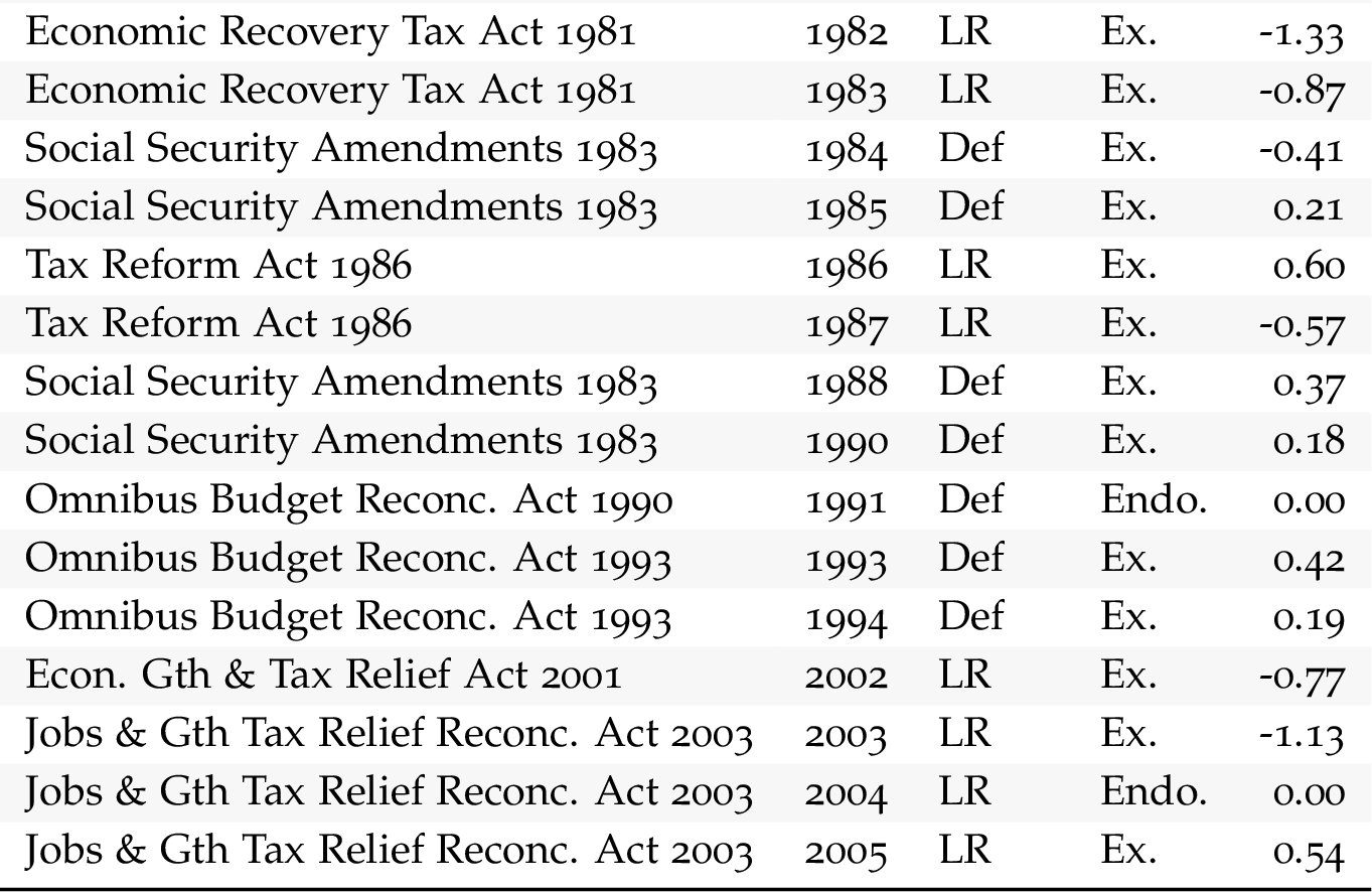
State their motivations:
Taxes raised to reduce the deficit, or increase long-run incentives are “exogenous.”
We do not want to look at tax changes which are made for managing the business cycle, in particular.
List of Tax Changes 1/2
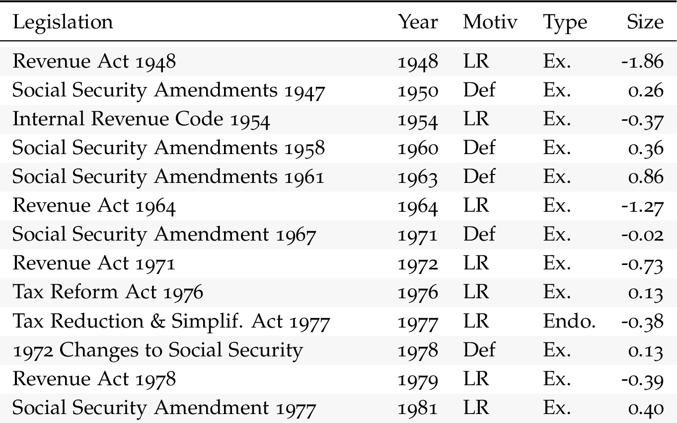
List of Tax Changes 2/2
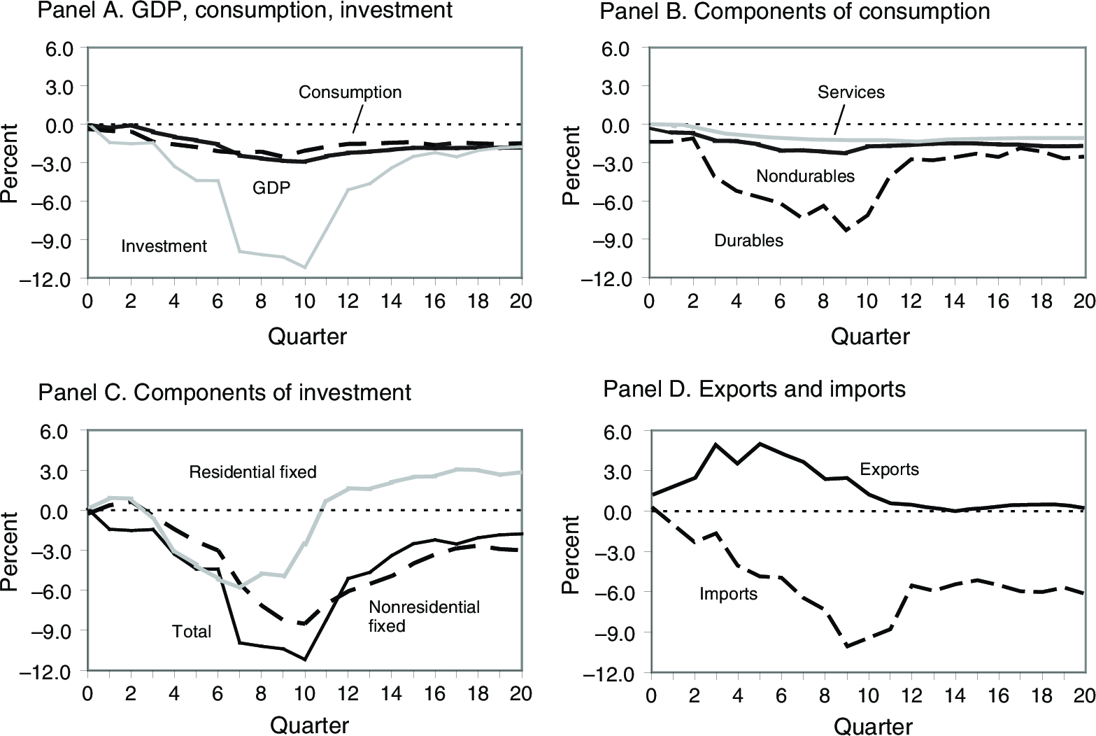
Tax Increase, 1% of GDP (Romer and Romer (2010))
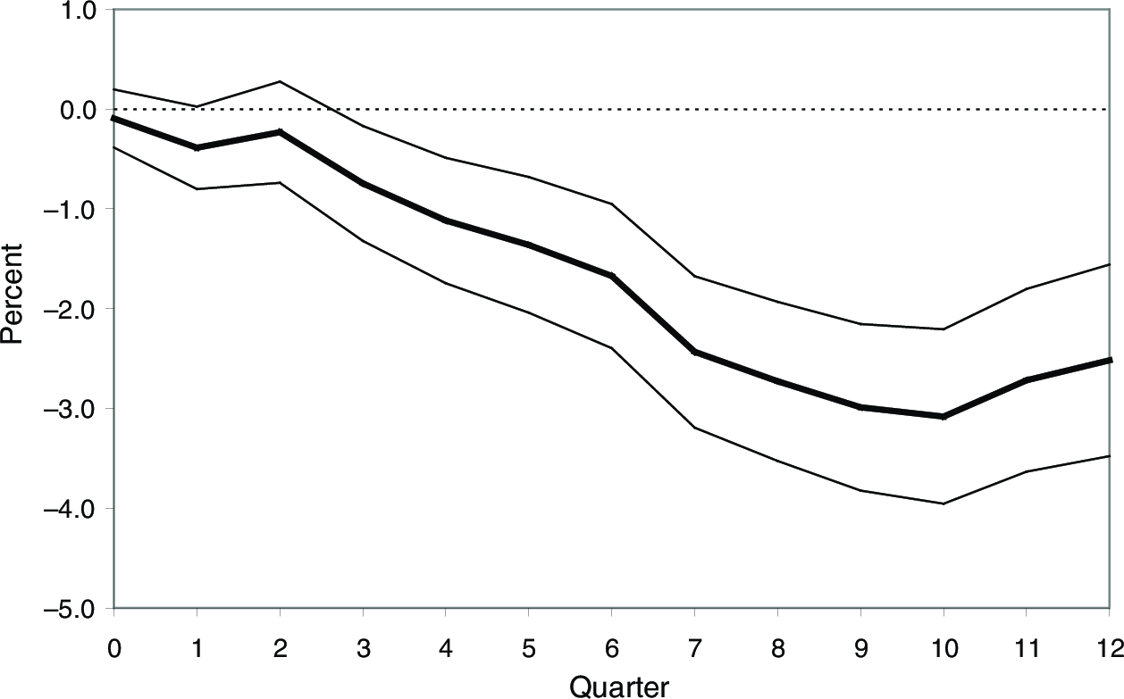
Romer and Romer (2010)
Advantages and Disadvantages
Issues with these studies:
– Noisy results: multiplier is between 2 and 4.
– One cannot further decompose: e.g. Top 10% VS Bottom 90%. We would get something even noisier.
– Always worry that tax changes are endogenous. (at the aggregate level, taxes are changed for a reason)
Advantages:
– It is exactly the object of interest (national level multiplier).
– Allows to tell apart different models.
Individual-Level Studies
Advantages and Disadvantages
Using individual-level data like survey, fiscal, administrative, or account-level data to measure \(\epsilon\), or \(c_{1}\). Advantages:
– Many more individuals: less noisy results (more observations).
– More credible “identification”: comparing two people at the same time period.
Disadvantages:
– Keynesian, aggregate demand effects cannot be estimated.
– e.g. if I decrease someone’s tax rate, then it might lead someone else to work more, not just the person who benefited from the fall in tax rates. (though the aggregate demand effect).
– Thus, there is no clean “control” group if there are aggregate demand effects.
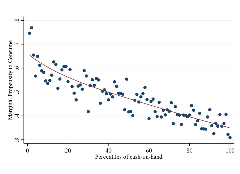
MPC (Jappelli and Pistaferri (2014))
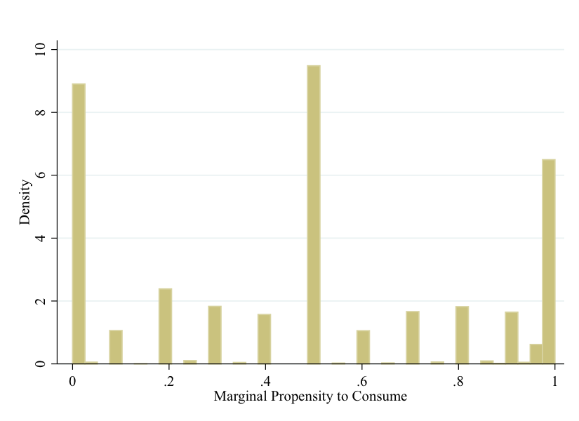
MPC (Jappelli and Pistaferri (2014))
Cross-sectional Studies
Advantages and Disadvantages
Identification across zipcodes, counties, or states. Advantages:
– More observations.
– Measure Keynesian, aggregate demand, general equilibrium effects.
– Less endogenous changes than at the national level: aggregate taxes are not changed in the U.S. to target California’s GDP specifically.
Disadvantages:
– Openness \(m_{1}\) of a state is larger, so multiplier is lower.
– But we are interested in national level multipliers, not state level multipliers.
– We thus need economic theory in order to infer national multipliers from state multipliers.
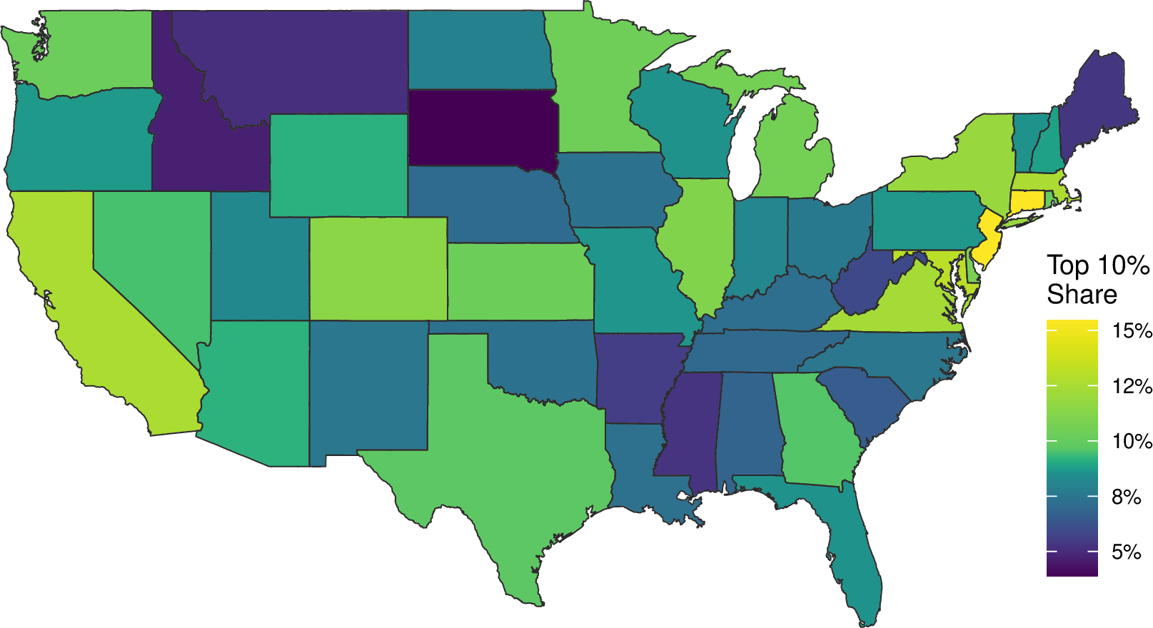
Zidar (2019): “Tax Cuts for Whom?”
Using state-level variation in income distributions, Zidar (2019) in a Journal of Political Economy paper named “Tax Cuts For Whom? Heterogeneous Effects of Income Tax Changes on Growth and Employment” estimates the following effects on GDP:
– Multiplier effect of a tax cut to the bottom 90% is roughly 7.
– Multiplier effect of a tax cut to the top 10% is roughly 0.
– A tax cut going half to both groups has a multiplier of about 3.5 (Romer, Romer (2010) result).
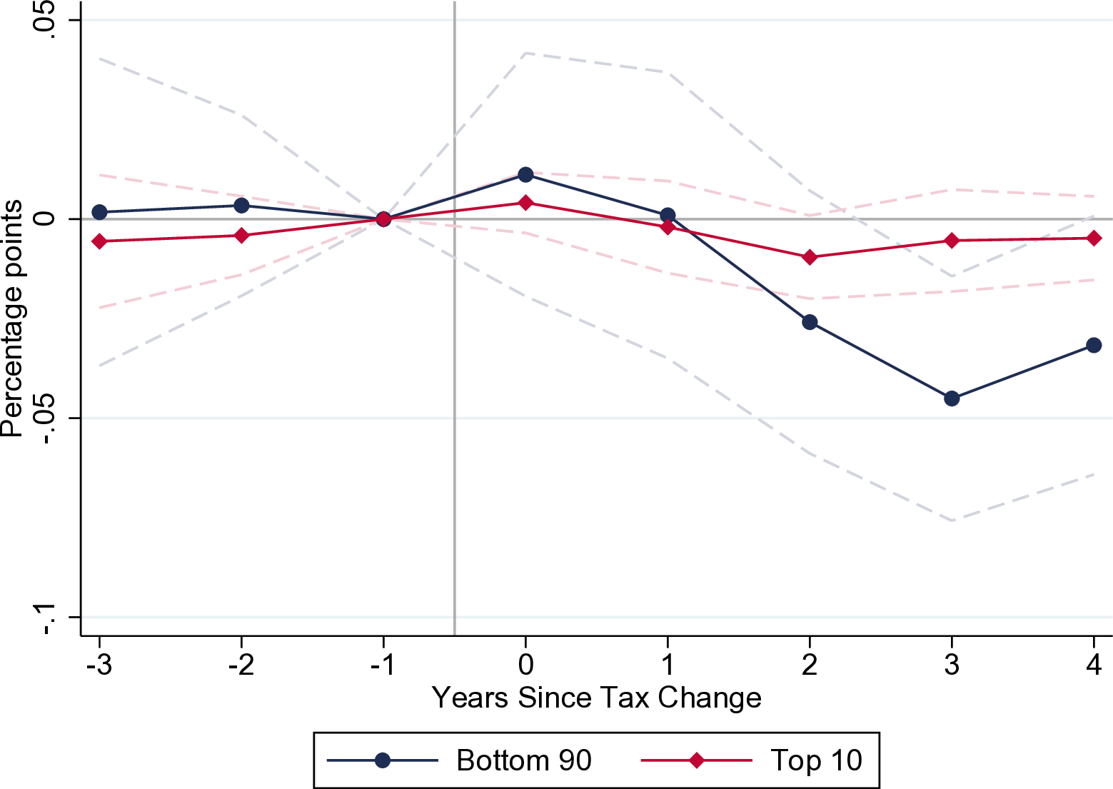
Zidar (2019): “Tax Cuts for Whom?”
Results seem to confirm our results from Lecture 9: tax cuts on bottom 90% work better than on top 10%.
Effects on employment are similar:
– 1% of state GDP tax cut for the bottom 90% results in 3.4% employment growth over a 2-year period.
– 1% of state GDP tax cut for the top 10% is 0.2% and statistically insignificant.
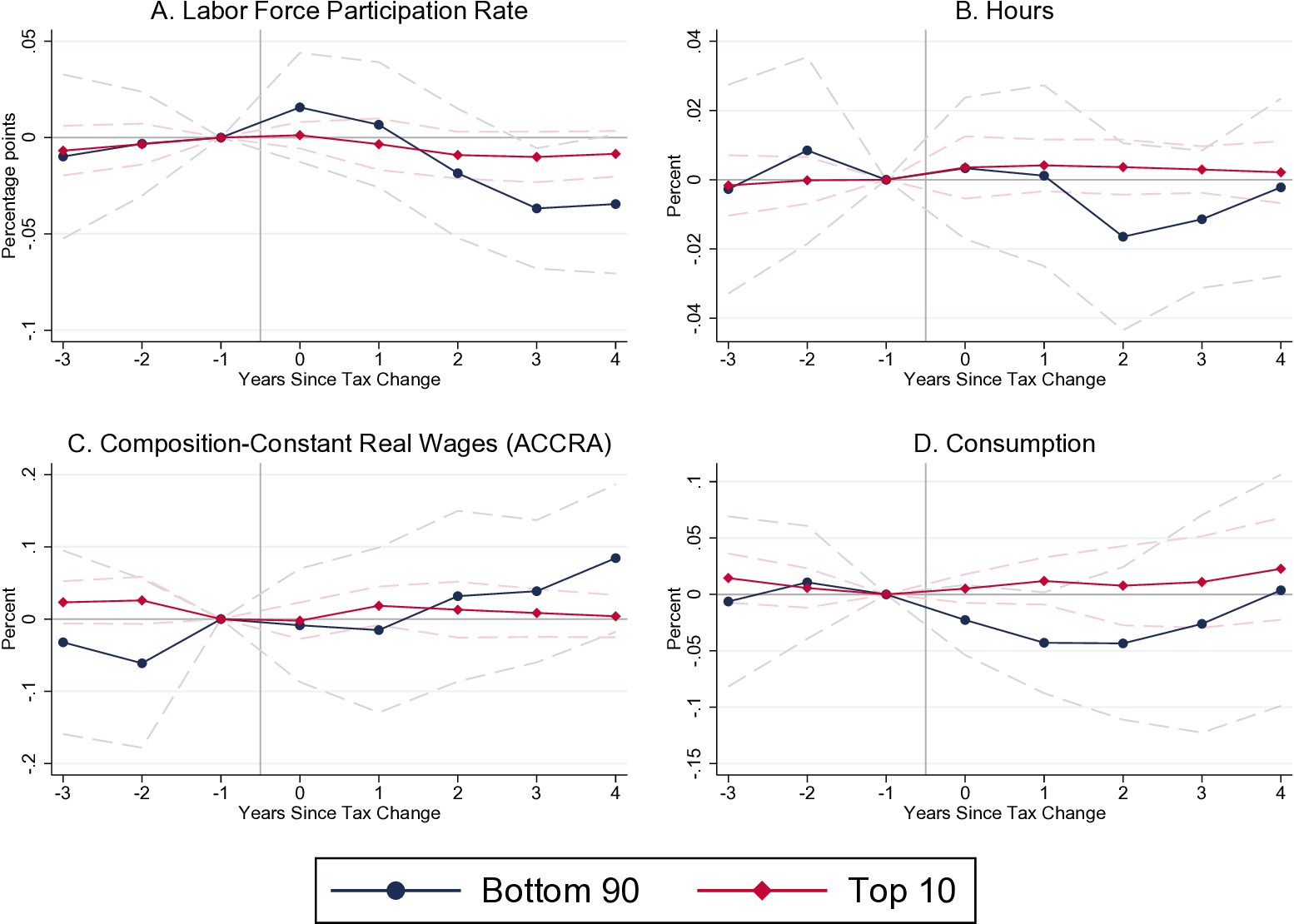
Zidar (2019)
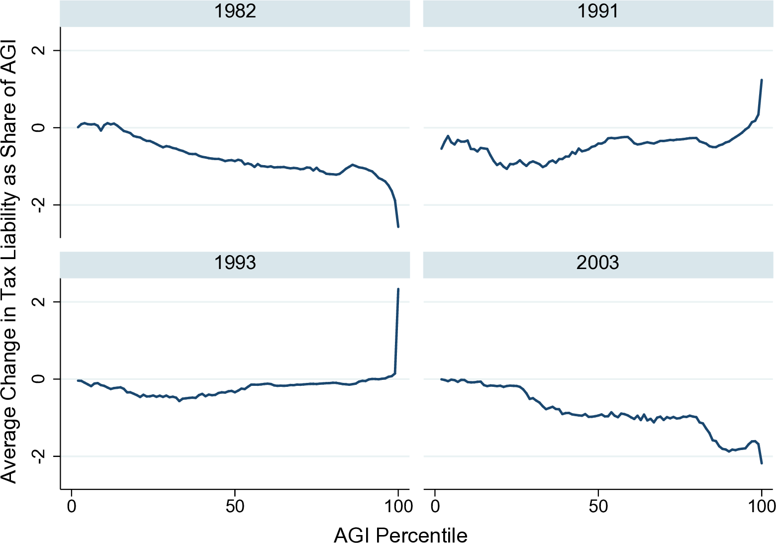
Zidar (2019)
Zidar (2019)
Zidar (2019)
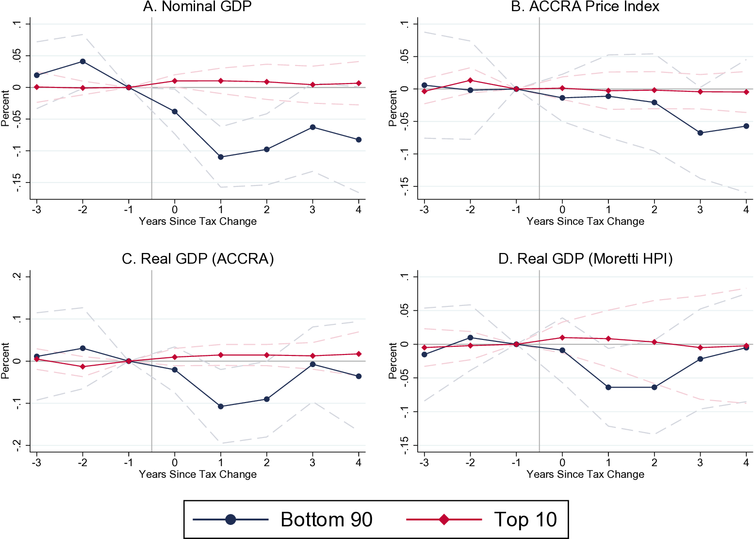
Zidar (2019)
Conclusion
Additional Watching (Not Required)
Taking Stock
Value of the Keynesian multiplier is still subject to very intense debates.
Tax-based multipliers > government spending multipliers (because tax changes are more persistent?)
Tax-based multipliers could be as high as 3.
Evidence that tax changes have long-term effect. There is a paradox of thrift.
My view: the evidence is more supportive of the Keynesian model, than of the neoclassical model.
Disclaimer: not everyone agrees with that view, and you are perfectly free to disagree too!
Bibliography
Hansen, Alvin H. 1939. “Economic Progress and Declining Population Growth.” The American Economic Review 29 (1): 1–15. http://www.jstor.org/stable/1806983.
Jappelli, Tullio, and Luigi Pistaferri. 2014. “Fiscal Policy and MPC Heterogeneity.” American Economic Journal: Macroeconomics 6 (4): 107–36. https://doi.org/10.1257/mac.6.4.107.
Keynes, John Maynard. 1936. The General Theory of Employment, Interest, and Money.
Romer, Christina D., and David H. Romer. 2010. “The Macroeconomic Effects of Tax Changes: Estimates Based on a New Measure of Fiscal Shocks.” American Economic Review 100 (3): 763–801. https://doi.org/10.1257/aer.100.3.763.
Zidar, Owen. 2019. “Tax Cuts for Whom? Heterogeneous Effects of Income Tax Changes on Growth and Employment.” Journal of Political Economy 127 (3): 1437–72. https://doi.org/10.1086/701424.