Lecture 6 - The Labor Market and Unemployment
Intermediate Macroeconomics - UCLA - Econ 102
François Geerolf
October 16, 2019
The Labor Market and Unemployment
Unemployment is no respecter of class or rank - Samuelson (1948)
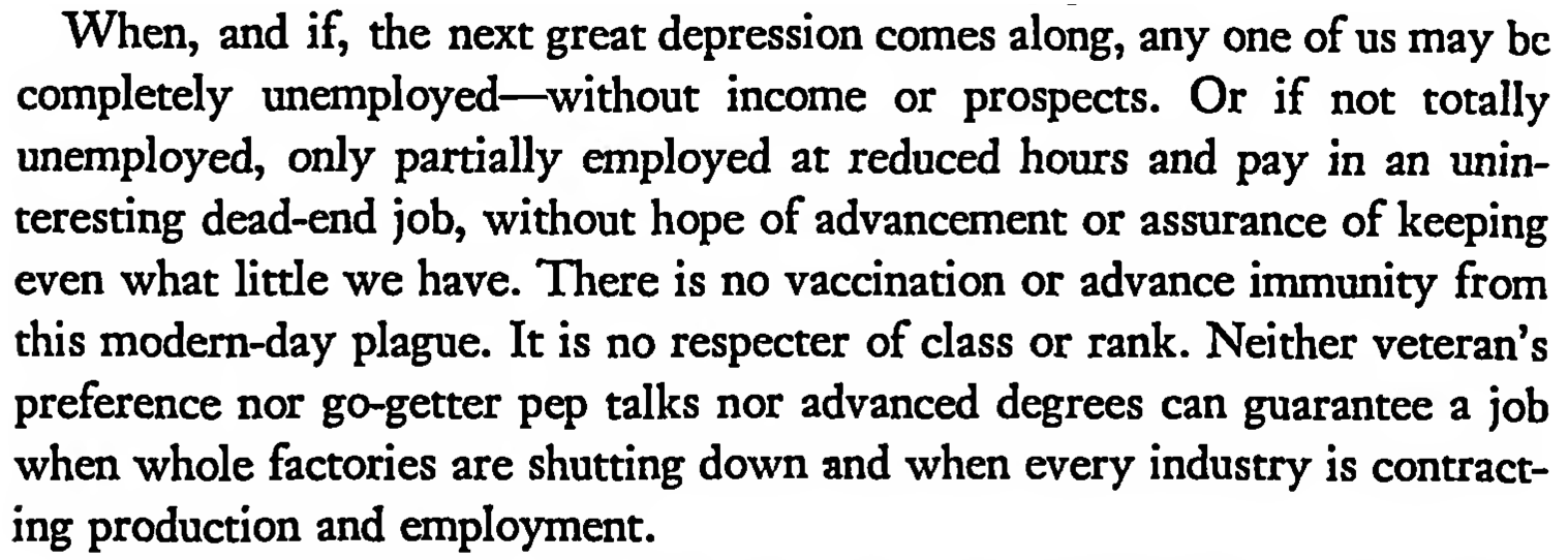
Unemployment is not only an economic problem - Samuelson (1948)
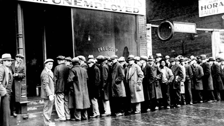
Free Soup
Please Give my Dad a Job

I only want one job

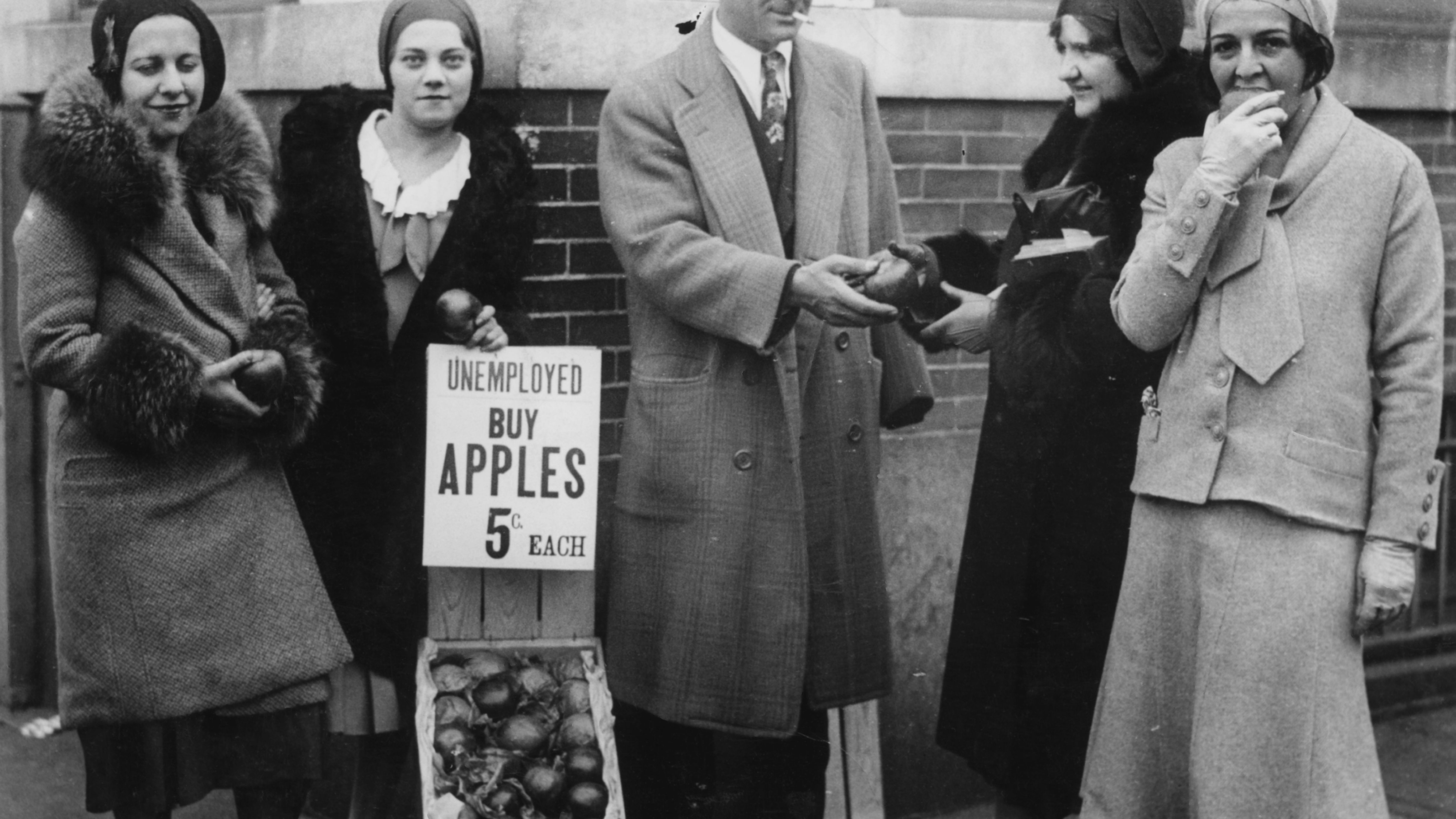
Buy apples
We want work

Buy tangerines

We can’t take care of our own

Free Food for Children of Unemployed

Neoclassical and Keynesian economics
This lecture on the labor market is a transition between neoclassical and Keynesian economics.
There are three views of the labor market:
A neoclassical view of the labor market: unemployment results from optimal market forces.
One “sticky-price”, “Keynesian” view of the labor market: wages and prices are “sticky”, and that is where involuntary unemployment comes from. Some people would like to work at the current wage but do not. Indeed, periods of high and persistent involuntary unemployment suggest that neoclassical economics is far from being the full story.
One over-saving, Keynesian view of the labor market: in the next few lectures, we shall develop a view of unemployment based on the imbalance between saving and investment what is called the “paradox of thrift.”
Data on Labor Market Slack
Several notions of labor market “slack”
There are many different notions of labor market “slack” (that is, people who would like to work but do not):
Unemployment Rate. Definitions vary across countries, and are not uncontroversial. (typically tied to unemployment benefits: are you looking for work?)
Labor Force Participation. Advantage is it does not rely on people’s statements. Disadvantage is it depends on how one defines the labor force (age), when people choose to retire, etc.
Prime-Age Labor Force Participation (25-54 years). This is less sensitive to how long people stay in college, and when they choose to retire.
All of this is however very debated.
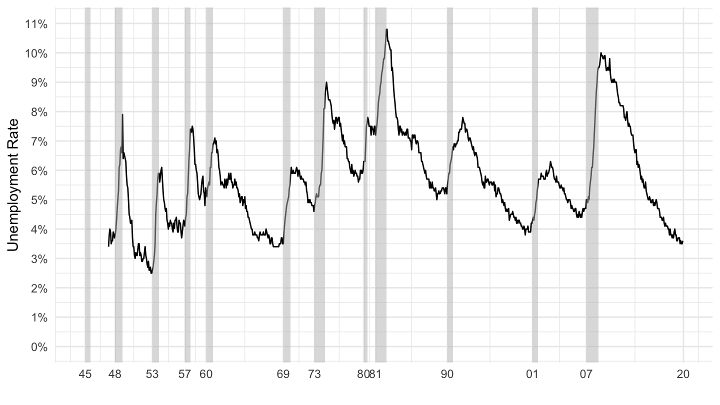
Unemployment Rate
Labor Force Participation

Labor Force Participation (25-54 years)

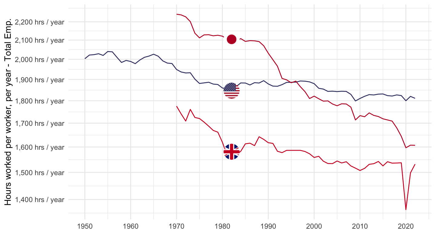
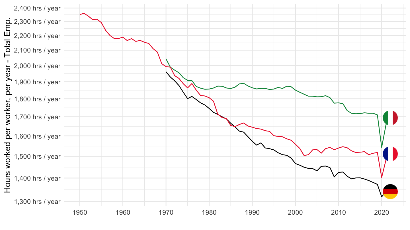
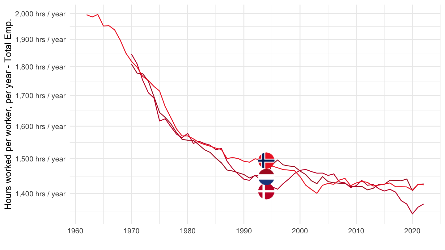
Hours of work per year
Japan, UK, US
France, Germany, Italy
Denmark, Netherlands, Norway
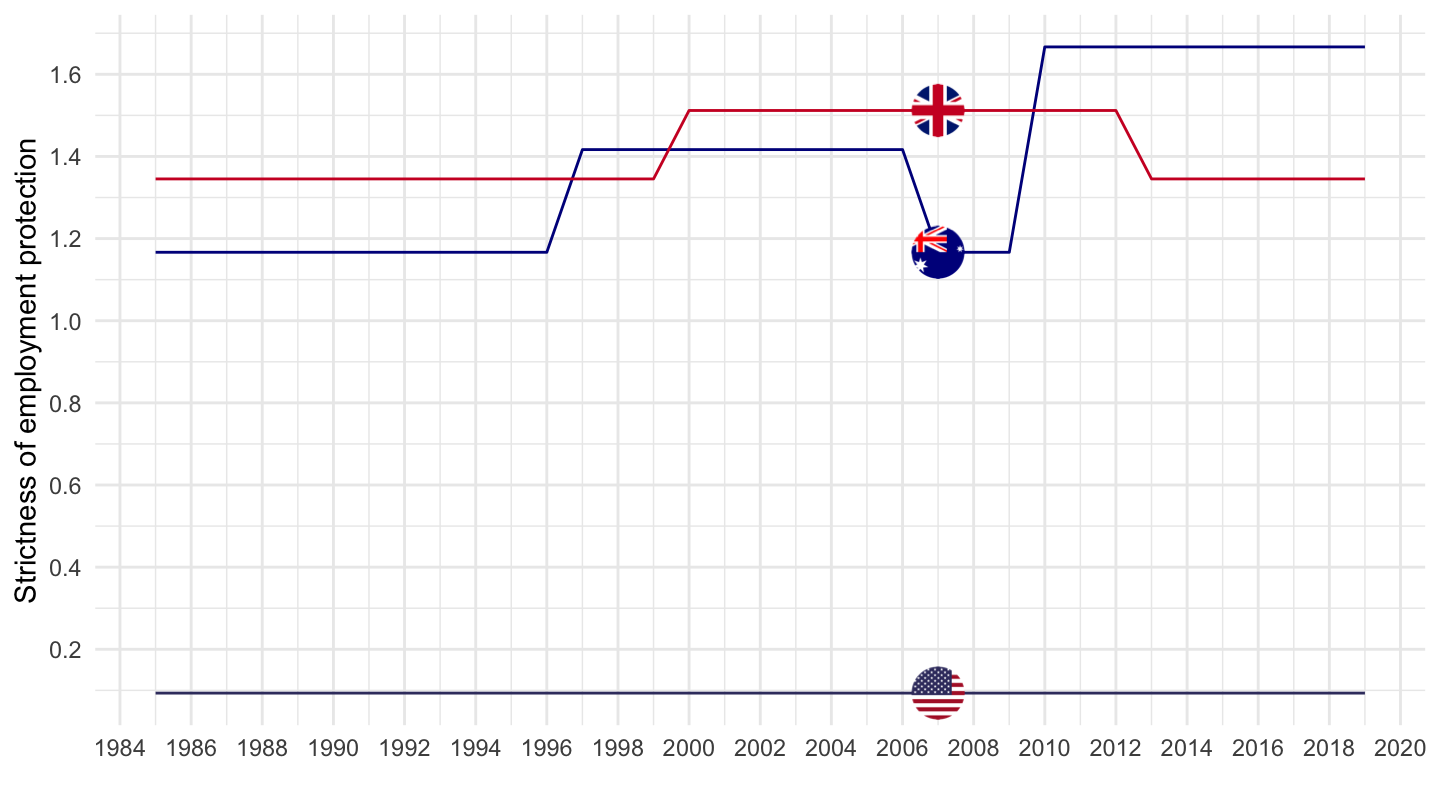
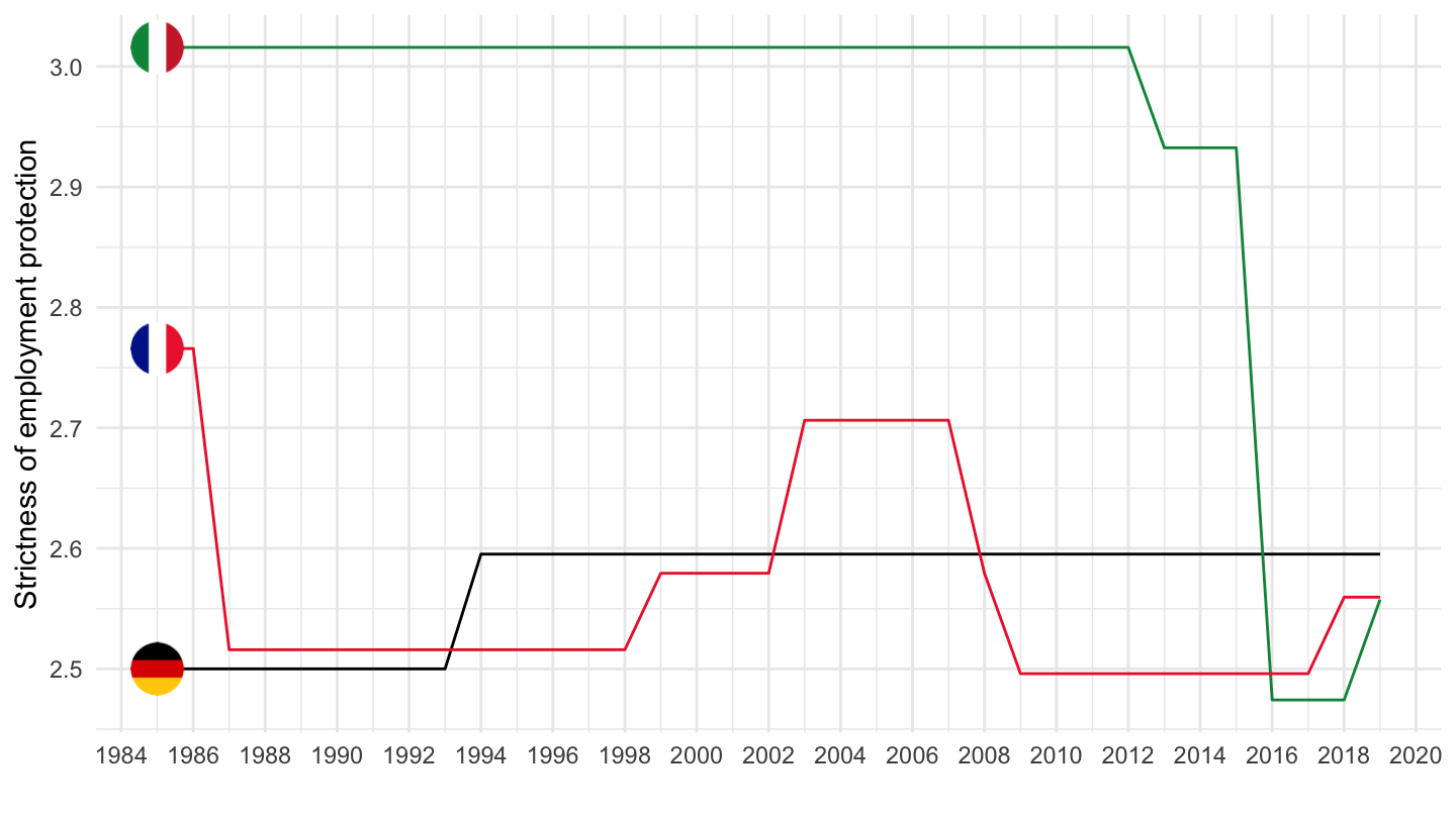
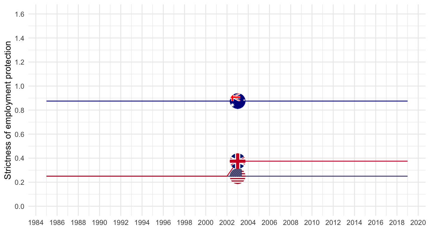
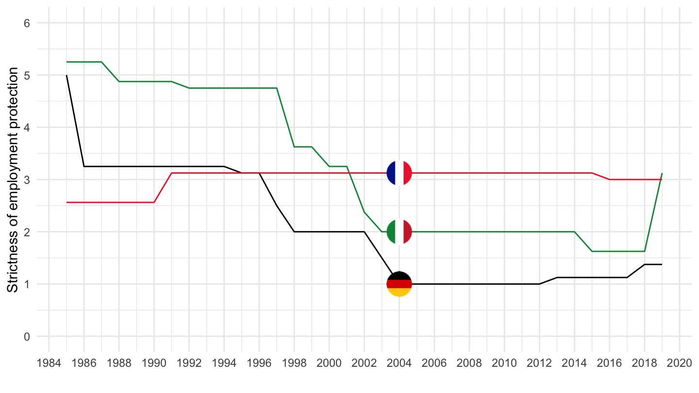
Strictness of Employment Protection
Regular Contracts: Anglo-Saxon
Regular Contracts: European
Temporary Contracts: Anglo-Saxon
Temporary Contracts: European
Labor Market Model
Labor Demand
Firms hire labor at price \(w\).
Sell the consumption good a price \(p\).
Assume decreasing returns to scale with respect to labor (think for example, that the quantity of capital is fixed): \[y = f(l).\]
Firms maximize their profits, and therefore solve: \[\max_l \quad pf(l) - wl.\]
Labor Supply: Assumptions
Neoclassical theory of labor supply starts from a static problem of a consumer-worker choosing how much to work, and how much to consume.
For example, assume that utility is strictly increasing in consumption, and strictly decreasing in the amount of labor supplied: \[U(c, l)=u(c)-v(l),\]
Budget constraint of a worker/consumer is given by: \[pc = wl.\]
Labor Supply: Assumptions
You may think of \(w\) as the hourly wage, for example $15/hour.
Then \(l\) would be expressed in terms of the number of hours.
Warning: Labor Supply and Labor Demand are sometimes being mixed up.
In the language of microeconomics, workers supply labor, and firms demand labor.
What workers do demand is jobs, or job vacancies, which are supplied by firms.
Fundamental postulate of neoclassical economics
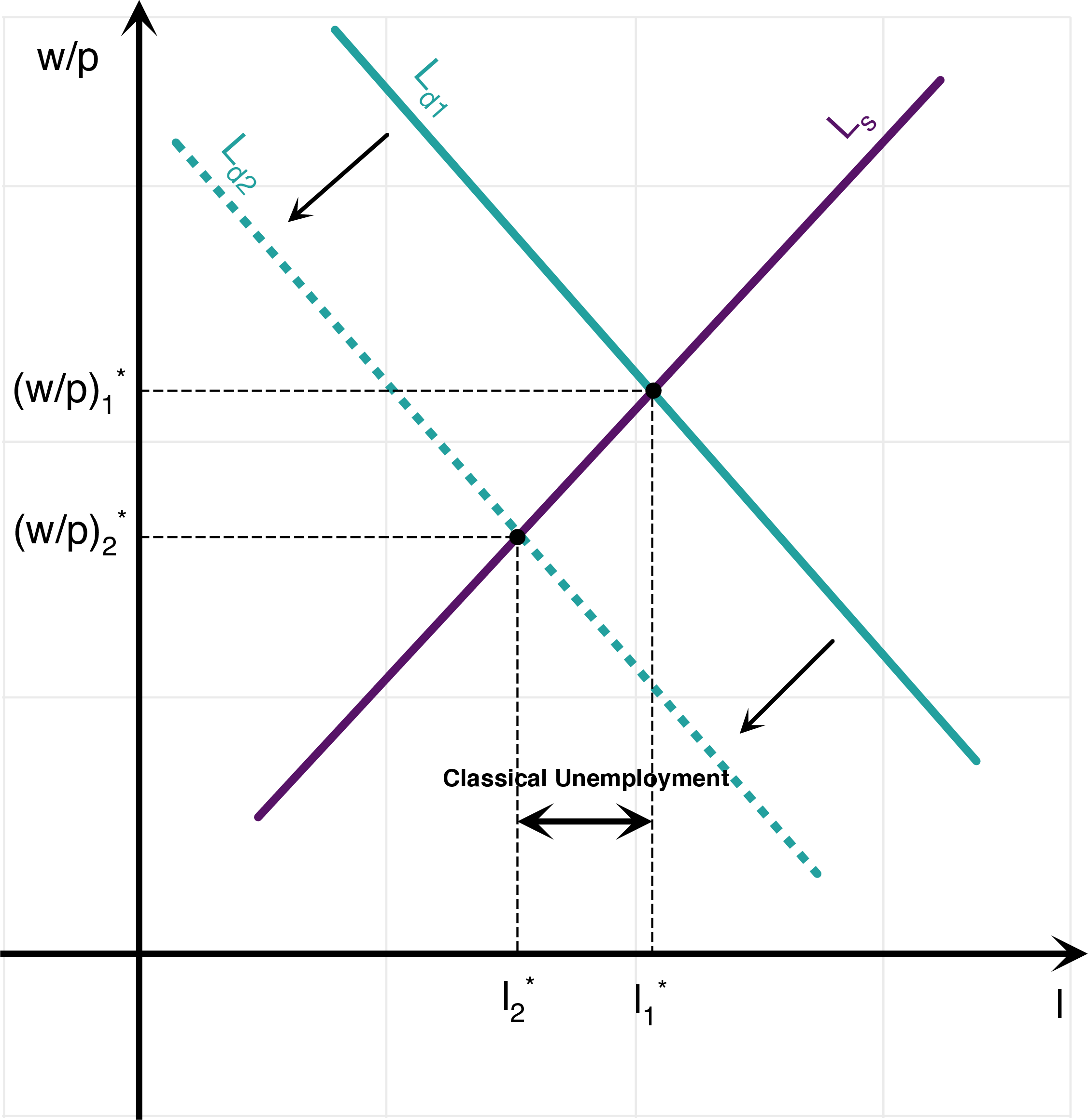
Labor demand shown above leads to the following first-order condition: \[pf'(l)-w = 0 \quad \Rightarrow \quad \boxed{f'(l)=\frac{w}{p}}.\]
Marginal product of labor (MPL) - that is, how much is gained from using one more unit of labor in production \(f'(l)\) - needs to be equal to how much that additional unit of labor costs to the firm, the real wage \(w/p\).
J.M. Keynes calls it the first fundamental postulate of classical economics in Chapter 2 of the General Theory. “The utility of the wage when a given volume of labour is employed is equal to the marginal disutility of that amount of employment.”
Fundamental postulate of neoclassical economics
- The problem of the consumer consists in maximizing utility under his budget constraint: \[ \begin{aligned} \max_{c,l}& \quad u(c)-v(l),\\ &\text{s.t.}\quad p \cdot c = w \cdot l. \end{aligned} \] Again, similarly to the consumption optimization problem, you may solve this optimization in four different ways.
Method 1
You may compute the ratio of marginal utilities (the marginal rate of substitution between consumption and labor).
State that it is equal to minus the real wage (because labor slackens the intertemporal budget constraint, and it appears on the right hand-side of the equal sign): \[\frac{\partial U / \partial l}{\partial U / \partial c} = -\frac{w}{p} \quad\Rightarrow\quad \boxed{\frac{v'(l)}{u'(c)}=\frac{w}{p}}\]
Method 2
You may apply the following intuitive economic argument.
The marginal disutility from supplying one more unit of labor is \(v'(l)\), for a worker already supplying \(l\) units of them. The marginal utility which is gained from doing so is given by the number of additional units of consumption one gets out of it, given by the real wage \(w/p\), and by how much I value each one of these additional utilities of consumption is valued, given by marginal utility \(u'(c)\).
The total gain in utility from consumption is the unit value \(u'(c)\) times the number of units \(w/p\), which gives the result: \[v'(l)=\frac{w}{p}u'(c)\quad \Rightarrow \quad \boxed{\frac{v'(l)}{u'(c)}=\frac{w}{p}.}\]
Method 3
You may substitute out \(l\) from the budget constraint, and optimize over the choice of consumption: \[\max_c \quad u(c)-v\left(\frac{p}{w} c\right).\]
This implies: \[u'(c)-\frac{p}{w}v'(l)=0 \quad \Rightarrow \quad \frac{v'(l)}{u'(c)}=\frac{w}{p}.\]
Method 4
You may substitute out \(c\) from the budget constraint, and optimize over the choice of labor: \[\max_l \quad u\left(\frac{w}{p}l\right)-v(l).\]
This implies: \[\frac{w}{l}u'(c)-v'(l)=0 \quad \Rightarrow \quad \boxed{\frac{v'(l)}{u'(c)}=\frac{w}{p}}.\]
Example
Assume a Cobb-Douglas production function for \(f(l)\), such that: \[f(l)=A l^{1-\alpha}.\]
Let us also assume linear utility for consumption (that is, people enjoy increasing utility equally, regardless of whether it is coming from the first dollar or the last one - this assumption is not realistic and is really made for simplicity), as well as a power function of disutility for work: \[u(c)=c, \quad v(l)=B\frac{l^{1+\epsilon}}{1+\epsilon}\]
Therefore: \[U(c, l)=c-B\frac{l^{1+\epsilon}}{1+\epsilon}.\]
Results 1/2
Using the above functional forms for \(u(.)\) and \(v(.)\) allows to write: \[v'(l)=Bl^{\epsilon}, \quad u'(c)=1, \quad \Rightarrow \quad Bl^{\epsilon} = \frac{w}{p}.\]
Labor supply \(L^{s}(.)\) as a function of the real wage \(w/p\) is thus given by: \[l =\frac{1}{B^{1/\epsilon}} \left(\frac{w}{p}\right)^{1/\epsilon} \equiv L^s\left(\frac{w}{p}\right).\]
Results 2/2
Moreover, using the above functional form for \(f(.)\) allows to write: \[f'(l) =A(1-\alpha)l^{-\alpha} \quad \Rightarrow \quad A(1-\alpha)l^{-\alpha}=\frac{w}{p}.\]
Labor demand \(L^d(.)\) is given as a function of the real wage \(w/p\) by: \[l=A^{1/\alpha}(1-\alpha)^{1/\alpha}\left(\frac{w}{p}\right)^{-1/\alpha}\equiv L^d\left(\frac{w}{p}\right).\]
Summing up
To sum up, the neoclassical labor market model is composed of the following labor supply and labor demand equations: \[ \begin{aligned} L^d\left(\frac{w}{p}\right) &= A^{1/\alpha}(1-\alpha)^{1/\alpha}\left(\frac{w}{p}\right)^{-1/\alpha},\\ L^s\left(\frac{w}{p}\right) &= \frac{1}{B^{1/\epsilon}} \left(\frac{w}{p}\right)^{1/\epsilon}. \end{aligned} \]
Market clearing implies that labor supply equals labor demand: \[ \begin{aligned} &L^d\left(\frac{w}{p}\right) = L^s\left(\frac{w}{p}\right) \\ & \quad \Rightarrow \quad \frac{w}{p} = (1-\alpha)^{\frac{\epsilon}{\alpha+\epsilon}}A^{\frac{\epsilon}{\alpha+\epsilon}} B^{\frac{\alpha}{\alpha+\epsilon}}. \end{aligned} \]
Results
- We may use either labor supply or labor demand in order to express the equilibrium quantity of labor \(l\). For example, let us use labor demand (as an exercise, you may check that using labor supply instead leads to the same expression): \[ \begin{aligned} l&=\frac{1}{B^{1/\epsilon}} \left(\frac{w}{p}\right)^{1/\epsilon}\\ &=\frac{1}{B^{1/\epsilon}} (1-\alpha)^{\frac{1}{\alpha+\epsilon}}A^{\frac{1}{\alpha+\epsilon}} B^{\frac{\alpha}{\epsilon(\alpha+\epsilon)}}\\ &= (1-\alpha)^{\frac{1}{\alpha+\epsilon}}A^{\frac{1}{\alpha+\epsilon}} B^{\frac{\alpha}{\epsilon(\alpha+\epsilon)}-\frac{1}{\epsilon}}\\ l&= (1-\alpha)^{\frac{1}{\alpha+\epsilon}}A^{\frac{1}{\alpha+\epsilon}} B^{-\frac{1}{\alpha+\epsilon}} \end{aligned} \]
Shock to Labor Demand
Neoclassical Model
“Keynesian” Model
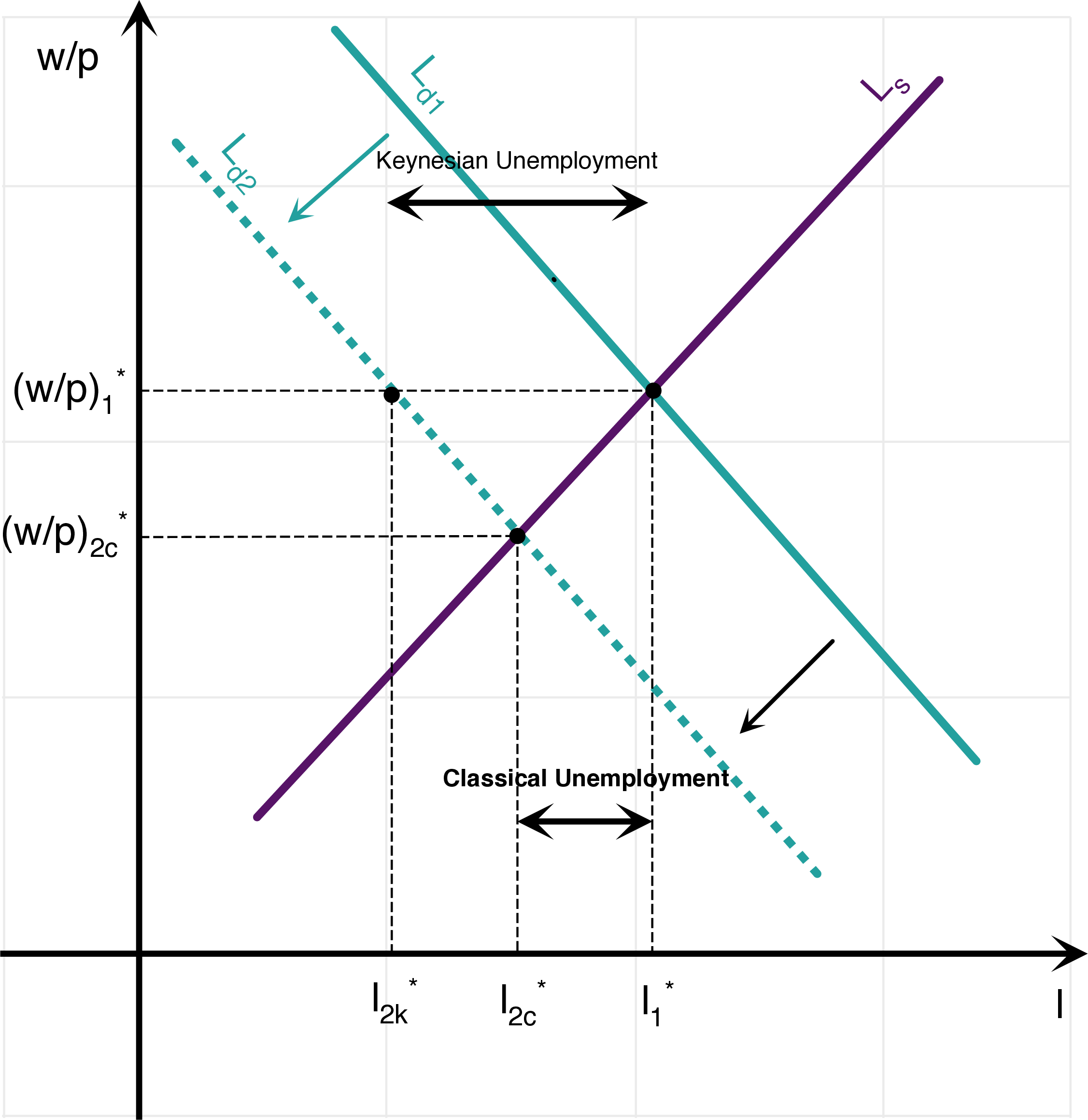
Why “Keynesian” - Leijonhufvud (1967)
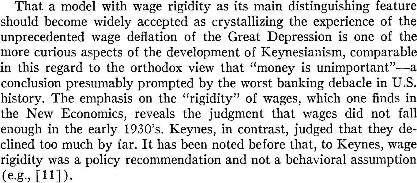
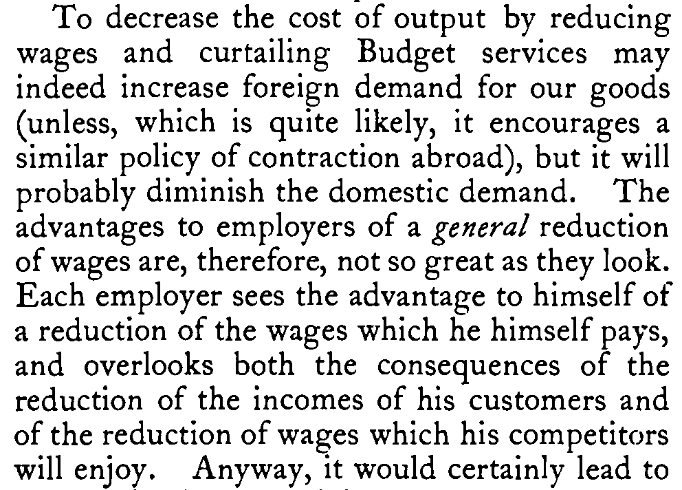
Keynes (1931) - on reducing wages
Data on Job Flows
Hires and Separations

Job Openings, Layoffs and Quits

Bibliography
Keynes, John Maynard. 1931. Essays in Persuasion. Springer.
Leijonhufvud, Axel. 1967. “Keynes and the Keynesians: A Suggested Interpretation.” The American Economic Review 57 (2): 401–10. https://www.jstor.org/stable/1821641.
Samuelson, Paul A. 1948. Economics. New York Toronto London: McGraw-Hill Book Company.