Indice de la production industrielle
Données - INSEE
Info
Info
- La nomenclature agrégée - NA, 2008. html
Données sur l’industrie
Code
industrie %>%
  arrange(-(dataset == "IPI-2021")) %>%
source_dataset_file_updates()| source | dataset | Title | .html | .rData |
|---|---|---|---|---|
| insee | IPI-2021 | Indice de la production industrielle | 2026-07-23 | 2026-07-23 |
| eurostat | mar_mg_am_cvh | Country level - volume (in TEUs) of containers handled in main ports, by loading status - mar_mg_am_cvh | 2026-07-23 | 2026-07-23 |
| eurostat | namq_10_a10 | Gross value added and income A*10 industry breakdowns | 2026-07-23 | 2026-07-23 |
| insee | CNA-2014-EMPLOI | Emploi intérieur, durée effective travaillée et productivité horaire | 2026-07-23 | 2026-07-22 |
| insee | CNT-2014-CB | Comptes des branches | 2026-07-23 | 2026-07-23 |
| insee | CNT-2014-OPERATIONS | Opérations sur biens et services | 2026-07-23 | 2026-07-23 |
| insee | ENQ-CONJ-ACT-IND | Conjoncture dans l’industrie | 2026-07-23 | 2026-07-23 |
| insee | ICA-2015-IND-CONS | Indices de chiffre d'affaires dans l'industrie et la construction | 2026-07-23 | 2026-07-23 |
| insee | IPPI-2015 | Indices de prix de production et d'importation dans l'industrie | 2026-07-23 | 2026-07-23 |
| insee | TCRED-EMPLOI-SALARIE-TRIM | Estimations d'emploi salarié par secteur d'activité et par département | 2026-07-23 | 2026-07-23 |
| insee | t_5407 | 5.407 – Solde extérieur de biens et de services par produit à prix courants (En milliards d'euros) - t_5407 | 2026-07-23 | 2021-08-01 |
| oecd | ALFS_EMP | Employment by activities and status (ALFS) | 2024-04-16 | 2025-05-24 |
| oecd | SNA_TABLE3 | Population and employment by main activity | 2024-09-15 | 2025-05-24 |
LAST_UPDATE
Code
`IPI-2021` %>%
  group_by(LAST_UPDATE) %>%
  summarise(Nobs = n()) %>%
  arrange(desc(LAST_UPDATE)) %>%
print_table_conditional()| LAST_UPDATE | Nobs |
|---|---|
| 2026-07-10 | 863 |
| 2026-07-03 | 323130 |
LAST_COMPILE
| LAST_COMPILE |
|---|
| 2026-07-24 |
Last
Code
`IPI-2021` %>%
  group_by(TIME_PERIOD) %>%
  summarise(Nobs = n()) %>%
  arrange(desc(TIME_PERIOD)) %>%
  head(1) %>%
print_table_conditional()| TIME_PERIOD | Nobs |
|---|---|
| 2026-05 | 730 |
Exemples
CORRECTION
Code
`IPI-2021` %>%
  left_join(CORRECTION, by = "CORRECTION") %>%
  group_by(CORRECTION, Correction) %>%
  summarise(Nobs = n()) %>%
  arrange(-Nobs) %>%
print_table_conditional()| CORRECTION | Correction | Nobs |
|---|---|---|
| BRUT | Non corrigé | 168094 |
| CVS-CJO | Corrigé des variations saisonnières et du nombre de jours ouvrables | 155899 |
NAF2
Tous
Code
`IPI-2021` %>%
  left_join(NAF2, by = "NAF2") %>%
  group_by(NAF2, Naf2) %>%
  summarise(Nobs = n()) %>%
  arrange(-Nobs) %>%
  print_table_conditional()
A10
Code
`IPI-2021` %>%
  filter(grepl("A10", NAF2)) %>%
  left_join(NAF2, by = "NAF2") %>%
  group_by(NAF2, Naf2) %>%
  summarise(Nobs = n()) %>%
  arrange(-Nobs) %>%
print_table_conditional()| NAF2 | Naf2 | Nobs |
|---|---|---|
| A10-CZ | A10-CZ - Industrie manufacturière | 1774 |
| A10-BE | A10-BE - Industrie manufacturière, industries extractives et autres | 911 |
| A10-FZ | A10-FZ - Construction | 37 |
A17
Code
`IPI-2021` %>%
  filter(grepl("A17", NAF2)) %>%
  left_join(NAF2, by = "NAF2") %>%
  group_by(NAF2, Naf2) %>%
  summarise(Nobs = n()) %>%
  arrange(-Nobs) %>%
print_table_conditional()| NAF2 | Naf2 | Nobs |
|---|---|---|
| A17-C1 | A17-C1 - Fabrication de denrées alimentaires, de boissons et de produits à base de tabac | 911 |
| A17-C2 | A17-C2 - Cokéfaction et raffinage | 911 |
| A17-C3 | A17-C3 - Fabrication d'équipements électriques, électroniques, informatiques ; fabrication de machines | 911 |
| A17-C4 | A17-C4 - Fabrication de matériels de transport | 911 |
| A17-C5 | A17-C5 - Fabrication d'autres produits industriels | 911 |
| A17-DE | A17-DE - Industries extractives, énergie, eau, gestion des déchets et dépollution | 911 |
A38
Code
`IPI-2021` %>%
  filter(grepl("A38", NAF2)) %>%
  left_join(NAF2, by = "NAF2") %>%
  group_by(NAF2, Naf2) %>%
  summarise(Nobs = n()) %>%
  arrange(-Nobs) %>%
print_table_conditional()| NAF2 | Naf2 | Nobs |
|---|---|---|
| A38-BZ | A38-BZ - Industries extractives | 911 |
| A38-CA | A38-CA - Fabrication de denrées alimentaires, de boissons et de produits à base de tabac | 911 |
| A38-CB | A38-CB - Fabrication de textiles, industries de l'habillement, industrie du cuir et de la chaussure | 911 |
| A38-CC | A38-CC - Travail du bois, industries du papier et imprimerie | 911 |
| A38-CD | A38-CD - Cokéfaction et raffinage | 911 |
| A38-CE | A38-CE - Industrie chimique | 911 |
| A38-CF | A38-CF - Industrie pharmaceutique | 911 |
| A38-CG | A38-CG - Fabrication de produits en caoutchouc et en plastique ainsi que d'autres produits minéraux non métalliques | 911 |
| A38-CH | A38-CH - Métallurgie et fabrication de produits métalliques à l'exception des machines et des équipements | 911 |
| A38-CI | A38-CI - Fabrication de produits informatiques, électroniques et optiques | 911 |
| A38-CJ | A38-CJ - Fabrication d'équipements électriques | 911 |
| A38-CK | A38-CK - Fabrication de machines et équipements n.c.a. | 911 |
| A38-CL | A38-CL - Fabrication de matériels de transport | 911 |
| A38-CM | A38-CM - Autres industries manufacturières ; réparation et installation de machines et d'équipements | 911 |
| A38-DZ | A38-DZ - Production et distribution d'électricité, de gaz, de vapeur et d'air conditionné | 911 |
| A38-EZ | A38-EZ - Production et distribution d'eau ; assainissement, gestion des déchets et dépollution | 911 |
A88
Code
`IPI-2021` %>%
  filter(nchar(NAF2) == 2) %>%
  left_join(NAF2, by = "NAF2") %>%
  group_by(NAF2, Naf2) %>%
  summarise(Nobs = n()) %>%
  arrange(-Nobs) %>%
print_table_conditional()| NAF2 | Naf2 | Nobs |
|---|---|---|
| SO | Sans objet | 7037 |
| 06 | 06 - Extraction d'hydrocarbures | 911 |
| 08 | 08 - Autres industries extractives | 911 |
| 10 | 10 - Industries alimentaires | 911 |
| 11 | 11 - Fabrication de boissons | 911 |
| 13 | 13 - Fabrication de textiles | 911 |
| 14 | 14 - Industrie de l'habillement | 911 |
| 15 | 15 - Industrie du cuir et de la chaussure | 911 |
| 16 | 16 - Travail du bois et fabrication d'articles en bois et en liège, à l'exception des meubles ; fabrication d'articles en vannerie et sparterie | 911 |
| 17 | 17 - Industrie du papier et du carton | 911 |
| 18 | 18 - Imprimerie et reproduction d'enregistrements | 911 |
| 19 | 19 - Cokéfaction et raffinage | 911 |
| 20 | 20 - Industrie chimique | 911 |
| 21 | 21 - Industrie pharmaceutique | 911 |
| 22 | 22 - Fabrication de produits en caoutchouc et en plastique | 911 |
| 23 | 23 - Fabrication d'autres produits minéraux non métalliques | 911 |
| 24 | 24 - Métallurgie | 911 |
| 25 | 25 - Fabrication de produits métalliques, à l'exception des machines et des équipements | 911 |
| 26 | 26 - Fabrication de produits informatiques, électroniques et optiques | 911 |
| 27 | 27 - Fabrication d'équipements électriques | 911 |
| 28 | 28 - Fabrication de machines et équipements n.c.a. | 911 |
| 29 | 29 - Industrie automobile | 911 |
| 30 | 30 - Fabrication d'autres matériels de transport | 911 |
| 31 | 31 - Fabrication de meubles | 911 |
| 32 | 32 - Autres industries manufacturières | 911 |
| 33 | 33 - Réparation et installation de machines et d'équipements | 911 |
| 35 | 35 - Production et distribution d'électricité, de gaz, de vapeur et d'air conditionné | 911 |
| 36 | 36 - Captage, traitement et distribution d'eau | 911 |
INDICATEUR
Code
`IPI-2021` %>%
  left_join(INDICATEUR, by = "INDICATEUR") %>%
  group_by(INDICATEUR, Indicateur) %>%
  summarise(Nobs = n()) %>%
  arrange(-Nobs) %>%
print_table_conditional()| INDICATEUR | Indicateur | Nobs |
|---|---|---|
| IPI | Indice de la production industrielle | 310935 |
| IPI_MOYENNE_ANNUELLE | Moyenne annuelle de l'indice de la production industrielle | 13058 |
FREQ
Code
`IPI-2021` %>%
  left_join(FREQ, by = "FREQ") %>%
  group_by(FREQ, Freq) %>%
  summarise(Nobs = n()) %>%
  arrange(-Nobs) %>%
print_table_conditional()| FREQ | Freq | Nobs |
|---|---|---|
| M | Monthly | 310935 |
| A | Annual | 13058 |
NATURE
Code
`IPI-2021` %>%
  left_join(NATURE, by = "NATURE") %>%
  group_by(NATURE, Nature) %>%
  summarise(Nobs = n()) %>%
  arrange(-Nobs) %>%
print_table_conditional()| NATURE | Nature | Nobs |
|---|---|---|
| INDICE | Indice | 310072 |
| MOYENNE_ANNUELLE | Moyenne annuelle | 13058 |
| VARIATIONS_M | Variations mensuelles | 437 |
| GLISSEMENT_ANNUEL | Glissement annuel | 426 |
TITLE_FR
Code
`IPI-2021` %>%
  group_by(IDBANK, TITLE_FR) %>%
  summarise(Nobs = n()) %>%
  arrange(-Nobs) %>%
  print_table_conditional()
TIME_PERIOD: 1990-
Code
`IPI-2021` %>%
  group_by(TIME_PERIOD) %>%
  summarise(Nobs = n()) %>%
  arrange(desc(TIME_PERIOD)) %>%
  print_table_conditional()
A10, A17
CZ, BE
Tous
Code
`IPI-2021` %>%
  filter(NAF2 %in% c("A10-CZ", "A10-BE"),
         CORRECTION == "CVS-CJO",
         NATURE == "INDICE") %>%
  left_join(NAF2, by = "NAF2") %>%
  select_if(function(col) length(unique(col)) > 1) %>%
  month_to_date %>%
  #filter(date >= as.Date("1995-01-01")) %>%
  mutate(OBS_VALUE = ifelse(year(date) == 2020 & month(date) %in% c(3, 4, 5, 6), NA, OBS_VALUE)) %>%
  group_by(Naf2) %>%
  mutate(OBS_VALUE = 100*OBS_VALUE/OBS_VALUE[date == as.Date("2020-02-01")]) %>%
  ggplot() + ylab("Indice de Production Industrielle vs. Février 2020\nhors Mars-Juin 2020") + xlab("") + theme_minimal() +
  geom_line(aes(x = date, y = OBS_VALUE, color = Naf2))  +
  geom_hline(yintercept = 100, linetype = "dashed") +

  scale_x_date(breaks = seq(1920, 2100, 5) %>% paste0("-01-01") %>% as.Date,
               labels = date_format("%Y")) +
  theme(legend.position = c(0.55, 0.15),
        legend.title = element_blank()) +
  scale_y_log10(breaks = seq(10, 120, 2),
                labels = percent(seq(10, 120, 2)/100 - 1, 1)) +
  geom_rect(data = data_frame(start = as.Date("2020-02-01"),
                                end = as.Date("2020-07-01")),
              aes(xmin = start, xmax = end, ymin = 0, ymax = +Inf), fill = viridis(4)[4], alpha = 0.2)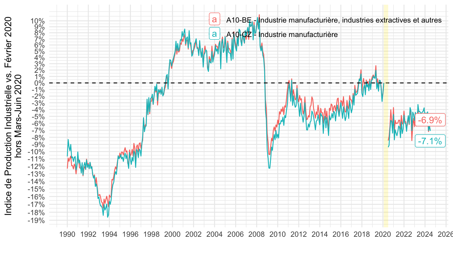
1995
Code
`IPI-2021` %>%
  filter(NAF2 %in% c("A10-CZ", "A10-BE"),
         CORRECTION == "CVS-CJO",
         NATURE == "INDICE") %>%
  left_join(NAF2, by = "NAF2") %>%
  select_if(function(col) length(unique(col)) > 1) %>%
  month_to_date %>%
  filter(date >= as.Date("1995-01-01")) %>%
  mutate(OBS_VALUE = ifelse(year(date) == 2020 & month(date) %in% c(3, 4, 5, 6), NA, OBS_VALUE)) %>%
  group_by(Naf2) %>%
  mutate(OBS_VALUE = 100*OBS_VALUE/OBS_VALUE[date == as.Date("2020-02-01")]) %>%
  ggplot() + ylab("Indice de Production Industrielle vs. Février 2020\nhors Mars-Juin 2020") + xlab("") + theme_minimal() +
  geom_line(aes(x = date, y = OBS_VALUE, color = Naf2))  +
  geom_label_repel(data = . %>%
              filter(date == max(date)), aes(x = date, y = OBS_VALUE, label = percent(OBS_VALUE/100-1, acc = .1), color = Naf2), show.legend = F) +
  geom_hline(yintercept = 100, linetype = "dashed") +

  scale_x_date(breaks = seq(1920, 2100, 2) %>% paste0("-01-01") %>% as.Date,
               labels = date_format("%Y")) +
  theme(legend.position = c(0.7, 0.9),
        legend.title = element_blank()) +
  scale_y_log10(breaks = seq(70, 110, 1),
                labels = percent(seq(70, 110, 1)/100 - 1, 1)) +
  geom_rect(data = data_frame(start = as.Date("2020-02-01"),
                                end = as.Date("2020-07-01")),
              aes(xmin = start, xmax = end, ymin = 0, ymax = +Inf), fill = viridis(4)[4], alpha = 0.2)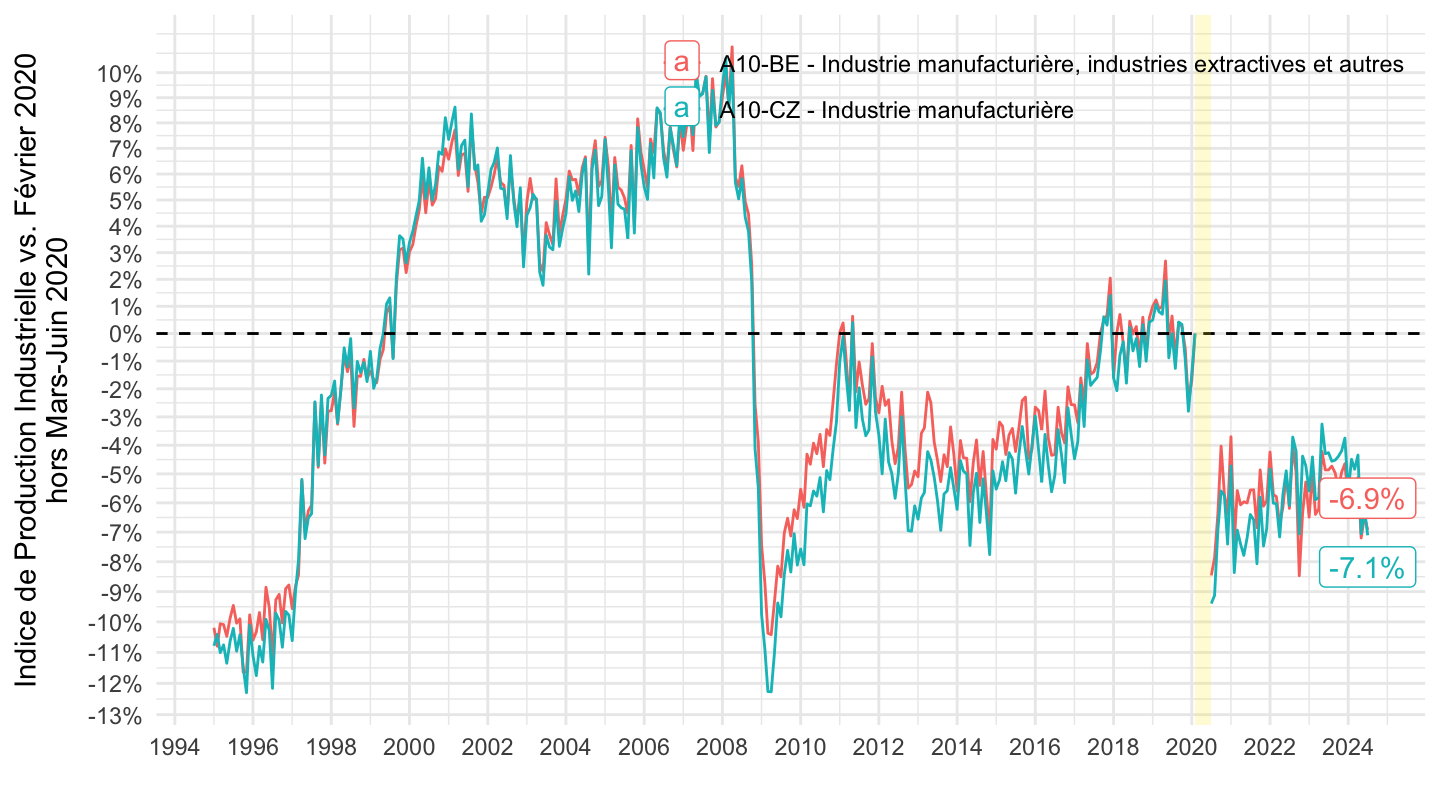
1999
Code
`IPI-2021` %>%
  filter(NAF2 %in% c("A10-CZ", "A10-BE"),
         CORRECTION == "CVS-CJO",
         NATURE == "INDICE") %>%
  left_join(NAF2, by = "NAF2") %>%
  select_if(function(col) length(unique(col)) > 1) %>%
  month_to_date %>%
  filter(date >= as.Date("1999-01-01")) %>%
  mutate(OBS_VALUE = ifelse(year(date) == 2020 & month(date) %in% c(3, 4, 5, 6), NA, OBS_VALUE)) %>%
  group_by(Naf2) %>%
  mutate(OBS_VALUE = 100*OBS_VALUE/OBS_VALUE[date == as.Date("2020-02-01")]) %>%
  ggplot() + ylab("Indice de Production Industrielle vs. Février 2020\nhors Mars-Juin 2020") + xlab("") + theme_minimal() +
  geom_line(aes(x = date, y = OBS_VALUE, color = Naf2))  +
  geom_label_repel(data = . %>%
              filter(date == max(date)), aes(x = date, y = OBS_VALUE, label = percent(OBS_VALUE/100-1, acc = .1), color = Naf2), show.legend = F) +
  geom_hline(yintercept = 100, linetype = "dashed") +

  scale_x_date(breaks = c(seq(1997, 2100, 5), seq(1999, 2100, 5)) %>% paste0("-01-01") %>% as.Date,
               labels = date_format("%Y")) +
  theme(legend.position = c(0.7, 0.9),
        legend.title = element_blank()) +
  scale_y_log10(breaks = seq(70, 110, 1),
                labels = percent(seq(70, 110, 1)/100 - 1, 1)) +
  geom_rect(data = data_frame(start = as.Date("2020-02-01"),
                                end = as.Date("2020-07-01")),
              aes(xmin = start, xmax = end, ymin = 0, ymax = +Inf), fill = viridis(4)[4], alpha = 0.2)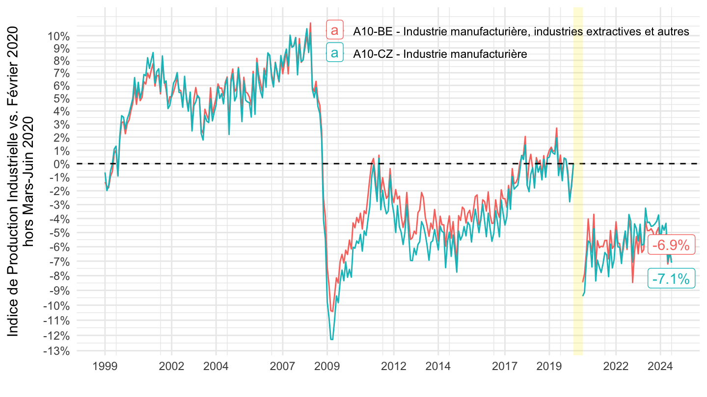
2000
Code
`IPI-2021` %>%
  filter(NAF2 %in% c("A10-CZ", "A10-BE"),
         CORRECTION == "CVS-CJO",
         NATURE == "INDICE") %>%
  left_join(NAF2, by = "NAF2") %>%
  select_if(function(col) length(unique(col)) > 1) %>%
  month_to_date %>%
  filter(date >= as.Date("2000-01-01")) %>%
  mutate(OBS_VALUE = ifelse(year(date) == 2020 & month(date) %in% c(3, 4, 5, 6), NA, OBS_VALUE)) %>%
  group_by(Naf2) %>%
  mutate(OBS_VALUE = 100*OBS_VALUE/OBS_VALUE[date == as.Date("2000-01-01")]) %>%
  ggplot() + ylab("Indice de Production Industrielle vs. Janvier 2000\n(hors Mars-Juin 2020)") + xlab("") + theme_minimal() +
  geom_line(aes(x = date, y = OBS_VALUE, color = Naf2))  +
  geom_label_repel(data = . %>%
              filter(date == max(date)), aes(x = date, y = OBS_VALUE, label = percent(OBS_VALUE/100-1, acc = .1), color = Naf2), show.legend = F) +
  geom_hline(yintercept = 100, linetype = "dashed") +

  scale_x_date(breaks = seq(1920, 2100, 2) %>% paste0("-01-01") %>% as.Date,
               labels = date_format("%Y")) +
  theme(legend.position = c(0.68, 0.9),
        legend.title = element_blank()) +
  scale_y_log10(breaks = seq(70, 120, 1)) +
  geom_rect(data = data_frame(start = as.Date("2020-02-01"),
                                end = as.Date("2020-07-01")),
              aes(xmin = start, xmax = end, ymin = 0, ymax = +Inf), fill = viridis(4)[4], alpha = 0.2)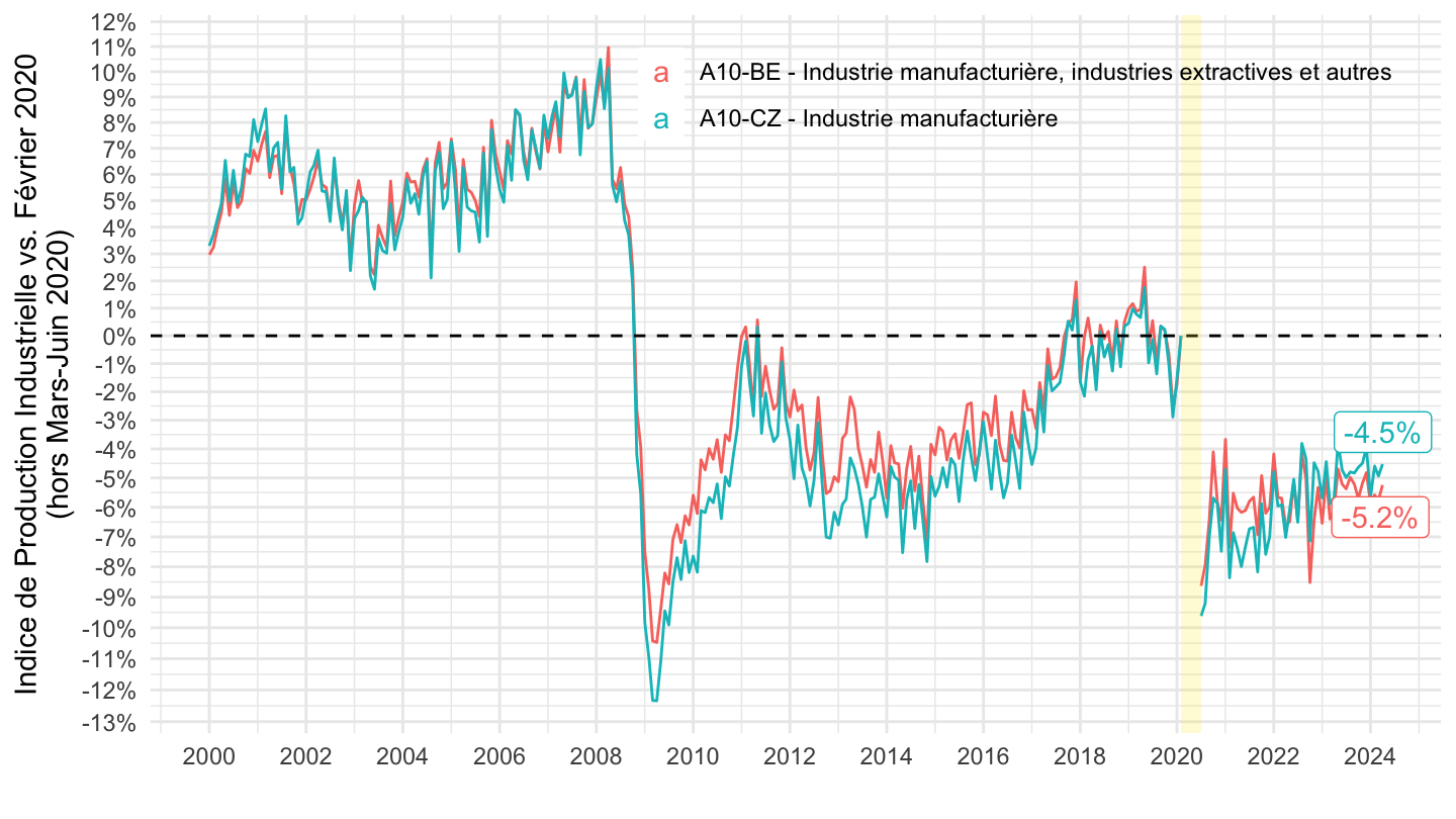
2005
Code
`IPI-2021` %>%
  filter(NAF2 %in% c("A10-CZ", "A10-BE"),
         CORRECTION == "CVS-CJO",
         NATURE == "INDICE") %>%
  left_join(NAF2, by = "NAF2") %>%
  select_if(function(col) length(unique(col)) > 1) %>%
  month_to_date %>%
  filter(date >= as.Date("2005-01-01")) %>%
  mutate(OBS_VALUE = ifelse(year(date) == 2020 & month(date) %in% c(3, 4, 5, 6), NA, OBS_VALUE)) %>%
  group_by(Naf2) %>%
  mutate(OBS_VALUE = 100*OBS_VALUE/OBS_VALUE[date == as.Date("2020-02-01")]) %>%
  ggplot() + ylab("Indice de Production Industrielle vs. Février 2020\nhors Mars-Juin 2020 (fermeture Covid-19)") + xlab("") + theme_minimal() +
  geom_line(aes(x = date, y = OBS_VALUE, color = Naf2))  +
  geom_label_repel(data = . %>%
              filter(date == max(date)), aes(x = date, y = OBS_VALUE, label = percent(OBS_VALUE/100-1, acc = .1), color = Naf2), show.legend = F) +
  geom_hline(yintercept = 100, linetype = "dashed") +

  scale_x_date(breaks = seq(1920, 2100, 1) %>% paste0("-01-01") %>% as.Date,
               labels = date_format("%Y")) +
  theme(legend.position = c(0.6, 0.9),
        legend.title = element_blank(),
        axis.text.x = element_text(angle = 45, vjust = 1, hjust=1)) +
  scale_y_log10(breaks = seq(80, 110, 1),
                labels = percent(seq(80, 110, 1)/100 - 1, 1)) +
  geom_rect(data = data_frame(start = as.Date("2020-02-01"),
                                end = as.Date("2020-07-01")),
              aes(xmin = start, xmax = end, ymin = 0, ymax = +Inf), fill = viridis(4)[4], alpha = 0.2)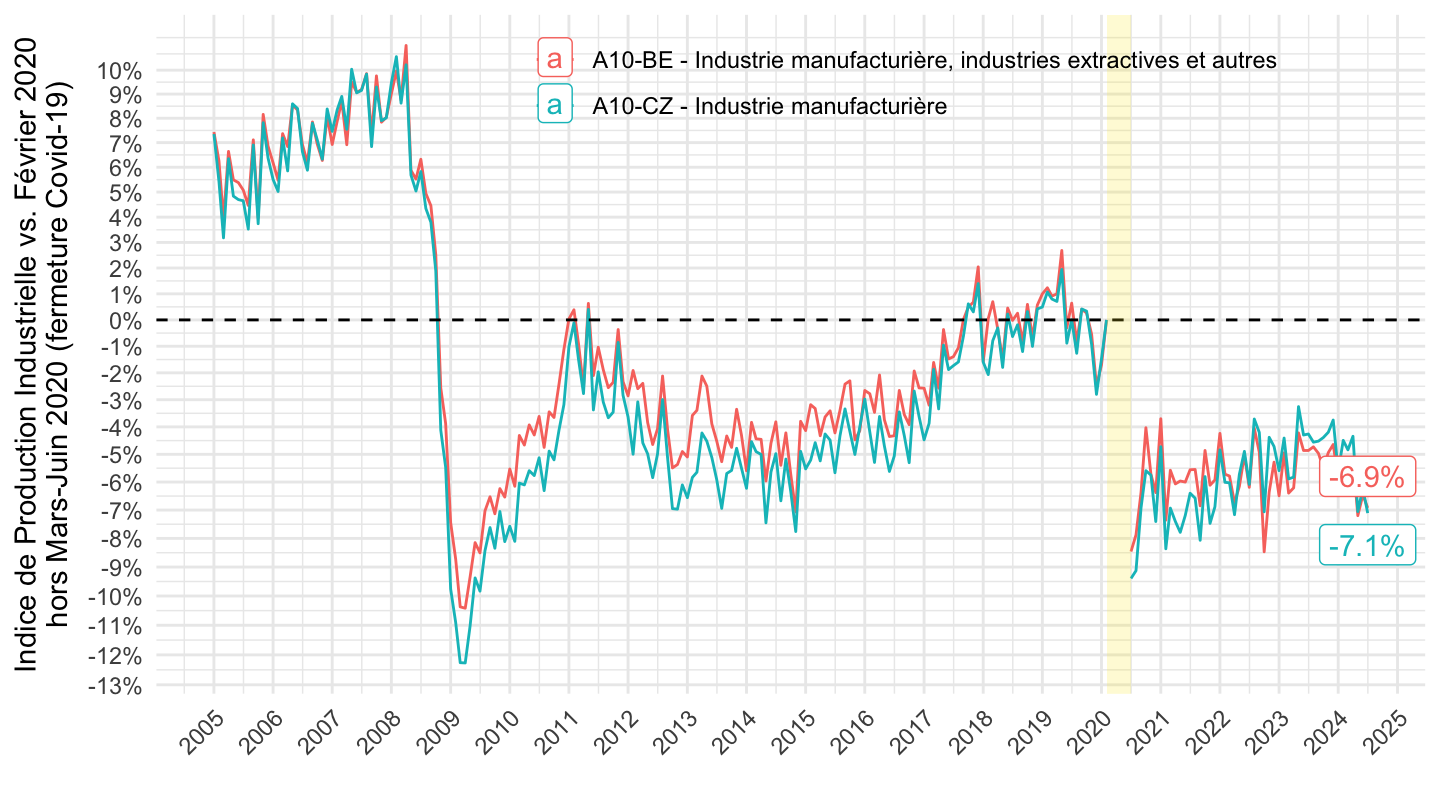
vs. 2008
Code
`IPI-2021` %>%
  filter(NAF2 %in% c("A10-CZ", "A10-BE"),
         CORRECTION == "CVS-CJO",
         NATURE == "INDICE") %>%
  left_join(NAF2, by = "NAF2") %>%
  select_if(function(col) length(unique(col)) > 1) %>%
  month_to_date %>%
  filter(date >= as.Date("2005-01-01")) %>%
  mutate(OBS_VALUE = ifelse(year(date) == 2020 & month(date) %in% c(3, 4, 5, 6), NA, OBS_VALUE)) %>%
  group_by(Naf2) %>%
  mutate(OBS_VALUE = 100*OBS_VALUE/OBS_VALUE[date == as.Date("2008-01-01")]) %>%
  ggplot() + ylab("Indice de Production Industrielle vs. Janvier 2008\nhors Mars-Juin 2020 (fermeture Covid-19)") + xlab("") + theme_minimal() +
  geom_line(aes(x = date, y = OBS_VALUE, color = Naf2))  +
  geom_text_repel(data = . %>%
              filter(date == max(date)), aes(x = date, y = OBS_VALUE, label = percent(OBS_VALUE/100-1, acc = .1), color = Naf2), show.legend = F) +
  geom_hline(yintercept = 100, linetype = "dashed") +

  scale_x_date(breaks = seq(1920, 2100, 1) %>% paste0("-01-01") %>% as.Date,
               labels = date_format("%Y")) +
  theme(legend.position = c(0.6, 0.8),
        legend.title = element_blank(),
        axis.text.x = element_text(angle = 45, vjust = 1, hjust=1)) +
  scale_y_log10(breaks = seq(80, 110, 1),
                labels = percent(seq(80, 110, 1)/100 - 1, 1)) +
  geom_rect(data = data_frame(start = as.Date("2020-02-01"),
                                end = as.Date("2020-07-01")),
              aes(xmin = start, xmax = end, ymin = 0, ymax = +Inf), fill = viridis(4)[4], alpha = 0.2)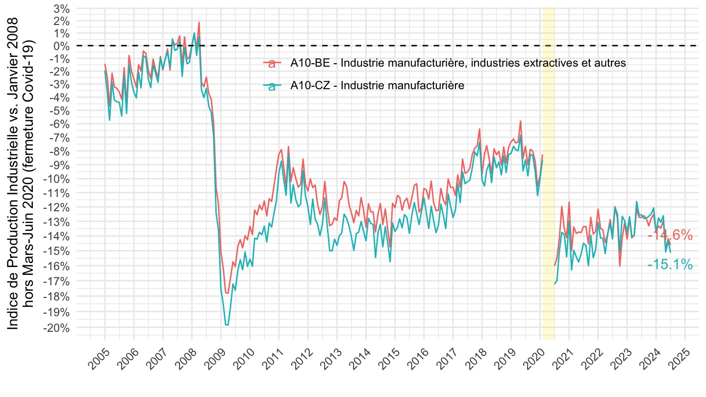
2010
Code
`IPI-2021` %>%
  filter(NAF2 %in% c("A10-CZ", "A10-BE"),
         CORRECTION == "CVS-CJO",
         NATURE == "INDICE") %>%
  left_join(NAF2, by = "NAF2") %>%
  select_if(function(col) length(unique(col)) > 1) %>%
  month_to_date %>%
  filter(date >= as.Date("2010-01-01")) %>%
  mutate(OBS_VALUE = ifelse(year(date) == 2020 & month(date) %in% c(3, 4, 5, 6), NA, OBS_VALUE)) %>%
  group_by(Naf2) %>%
  mutate(OBS_VALUE = 100*OBS_VALUE/OBS_VALUE[date == as.Date("2020-02-01")]) %>%
  ggplot() + ylab("Indice de Production Industrielle vs. Février 2020\nhors Mars-Juin 2020") + xlab("") + theme_minimal() +
  geom_line(aes(x = date, y = OBS_VALUE, color = Naf2))  +
  geom_label_repel(data = . %>%
              filter(date == max(date)), aes(x = date, y = OBS_VALUE, label = percent(OBS_VALUE/100-1, acc = .1), color = Naf2), show.legend = F) +
  geom_hline(yintercept = 100, linetype = "dashed") +

  scale_x_date(breaks = seq(1920, 2100, 1) %>% paste0("-01-01") %>% as.Date,
               labels = date_format("%Y")) +
  theme(legend.position = c(0.3, 0.9),
        legend.title = element_blank()) +
  scale_y_log10(breaks = seq(90, 110, 1),
                labels = percent(seq(90, 110, 1)/100 - 1, 1)) +
  geom_rect(data = data_frame(start = as.Date("2020-02-01"),
                                end = as.Date("2020-07-01")),
              aes(xmin = start, xmax = end, ymin = 0, ymax = +Inf), fill = viridis(4)[4], alpha = 0.2)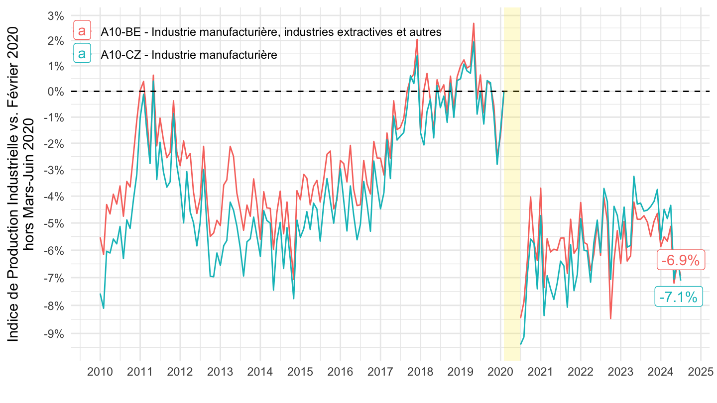
2015-
Code
`IPI-2021` %>%
  filter(NAF2 %in% c("A10-CZ", "A10-BE"),
         CORRECTION == "CVS-CJO",
         NATURE == "INDICE") %>%
  left_join(NAF2, by = "NAF2") %>%
  select_if(function(col) length(unique(col)) > 1) %>%
  month_to_date %>%
  filter(date >= as.Date("2015-01-01")) %>%
  mutate(OBS_VALUE = ifelse(year(date) == 2020 & month(date) %in% c(3, 4, 5, 6), NA, OBS_VALUE)) %>%
  group_by(Naf2) %>%
  mutate(OBS_VALUE = 100*OBS_VALUE/OBS_VALUE[date == as.Date("2020-02-01")]) %>%
  ggplot() + ylab("Indice de Production Industrielle vs. Février 2020\nhors Mars-Juin 2020") + xlab("") + theme_minimal() +
  geom_line(aes(x = date, y = OBS_VALUE, color = Naf2), size = 1)  +
  geom_text_repel(data = . %>%
              filter(date == max(date)), aes(x = date, y = OBS_VALUE, label = percent(OBS_VALUE/100-1, acc = .1), color = Naf2), show.legend = F, point.padding = 10) +
  geom_hline(yintercept = 100, linetype = "dashed") +

  scale_x_date(breaks = seq(1920, 2100, 1) %>% paste0("-01-01") %>% as.Date,
               labels = date_format("%Y")) +
  theme(legend.position = c(0.4, 0.95),
        legend.title = element_blank()) +
  scale_y_log10(breaks = seq(90, 110, 1),
                labels = percent(seq(90, 110, 1)/100 - 1, 1)) +
  geom_rect(data = data_frame(start = as.Date("2020-02-01"),
                                end = as.Date("2020-07-01")),
              aes(xmin = start, xmax = end, ymin = 0, ymax = +Inf), fill = viridis(4)[4], alpha = 0.2)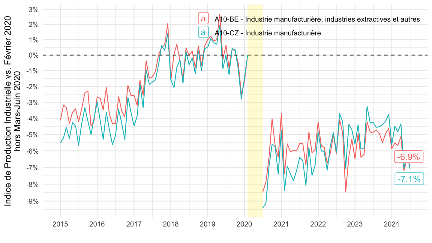
Mai 2017-
Code
`IPI-2021` %>%
  filter(NAF2 %in% c("A10-CZ", "A10-BE"),
         CORRECTION == "CVS-CJO",
         NATURE == "INDICE") %>%
  left_join(NAF2, by = "NAF2") %>%
  select_if(function(col) length(unique(col)) > 1) %>%
  month_to_date %>%
  arrange(desc(date)) %>%
  filter(date >= as.Date("2017-05-01")) %>%
  mutate(OBS_VALUE = ifelse(year(date) == 2020 & month(date) %in% c(3, 4, 5, 6), NA, OBS_VALUE)) %>%
  group_by(Naf2) %>%
  mutate(OBS_VALUE = 100*OBS_VALUE/OBS_VALUE[date == as.Date("2017-05-01")]) %>%
  ggplot() + ylab("Indice de Production Industrielle vs. Mai 2017\nhors Mars-Juin 2020") + xlab("") + theme_minimal() +
  geom_line(aes(x = date, y = OBS_VALUE, color = Naf2), size = 1)  +
  geom_label_repel(data = . %>%
              filter(date == max(date)), aes(x = date, y = OBS_VALUE, label = percent(OBS_VALUE/100-1, acc = .1), color = Naf2), show.legend = F) +
  geom_hline(yintercept = 100, linetype = "dashed") +

  scale_x_date(breaks = seq(1920, 2100, 1) %>% paste0("-01-01") %>% as.Date,
               labels = date_format("%Y")) +
  theme(legend.position = c(0.65, 0.9),
        legend.title = element_blank()) +
  scale_y_log10(breaks = seq(90, 110, 1),
                labels = percent(seq(90, 110, 1)/100 - 1, 1)) +
  geom_rect(data = data_frame(start = as.Date("2020-02-01"),
                                end = as.Date("2020-07-01")),
              aes(xmin = start, xmax = end, ymin = 0, ymax = +Inf), fill = viridis(4)[4], alpha = 0.2)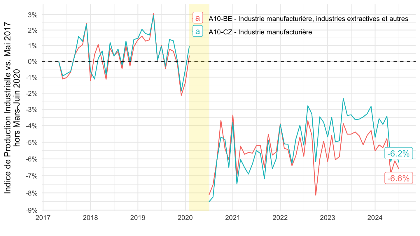
2018
Code
`IPI-2021` %>%
  filter(NAF2 %in% c("A10-CZ", "A10-BE"),
         CORRECTION == "CVS-CJO",
         NATURE == "INDICE") %>%
  left_join(NAF2, by = "NAF2") %>%
  select_if(function(col) length(unique(col)) > 1) %>%
  month_to_date %>%
  filter(date >= as.Date("2018-01-01")) %>%
  mutate(OBS_VALUE = ifelse(year(date) == 2020 & month(date) %in% c(3, 4, 5, 6), NA, OBS_VALUE)) %>%
  group_by(Naf2) %>%
  mutate(OBS_VALUE = 100*OBS_VALUE/OBS_VALUE[date == as.Date("2020-02-01")]) %>%
  ggplot() + ylab("Indice de Production Industrielle vs. Février 2020\nhors Mars-Juin 2020") + xlab("") + theme_minimal() +
  geom_line(aes(x = date, y = OBS_VALUE, color = Naf2), size = 1)  +
  geom_label_repel(data = . %>%
              filter(date == max(date)), aes(x = date, y = OBS_VALUE, label = percent(OBS_VALUE/100-1, acc = .1), color = Naf2), show.legend = F) +
  geom_hline(yintercept = 100, linetype = "dashed") +

  scale_x_date(breaks = seq(1920, 2100, 1) %>% paste0("-01-01") %>% as.Date,
               labels = date_format("%Y")) +
  theme(legend.position = c(0.6, 0.9),
        legend.title = element_blank()) +
  scale_y_log10(breaks = seq(90, 110, 1),
                labels = percent(seq(90, 110, 1)/100 - 1, 1)) +
  geom_rect(data = data_frame(start = as.Date("2020-02-01"),
                                end = as.Date("2020-07-01")),
              aes(xmin = start, xmax = end, ymin = 0, ymax = +Inf), fill = viridis(4)[4], alpha = 0.2)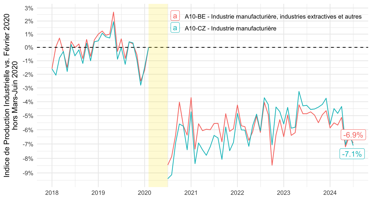
vs. janvier 2020
Code
`IPI-2021` %>%
  filter(NAF2 %in% c("A10-CZ", "A10-BE"),
         CORRECTION == "CVS-CJO",
         NATURE == "INDICE") %>%
  left_join(NAF2, by = "NAF2") %>%
  select_if(function(col) length(unique(col)) > 1) %>%
  month_to_date %>%
  filter(date >= as.Date("2018-01-01")) %>%
  mutate(OBS_VALUE = ifelse(year(date) == 2020 & month(date) %in% c(3, 4, 5, 6), NA, OBS_VALUE)) %>%
  group_by(Naf2) %>%
  mutate(OBS_VALUE = 100*OBS_VALUE/OBS_VALUE[date == as.Date("2020-02-01")]) %>%
  ggplot() + ylab("Indice de Production Industrielle vs. Février 2020\nhors Mars-Juin 2020") + xlab("") + theme_minimal() +
  geom_line(aes(x = date, y = OBS_VALUE, color = Naf2))  +
  geom_label_repel(data = . %>%
              filter(date == max(date)), aes(x = date, y = OBS_VALUE, label = percent(OBS_VALUE/100-1, acc = .1), color = Naf2), show.legend = F) +
  geom_hline(yintercept = 100, linetype = "dashed") +

  scale_x_date(breaks = seq(1920, 2100, 1) %>% paste0("-01-01") %>% as.Date,
               labels = date_format("%Y")) +
  theme(legend.position = c(0.7, 0.9),
        legend.title = element_blank()) +
  scale_y_log10(breaks = seq(90, 110, 1),
                labels = percent(seq(90, 110, 1)/100 - 1, 1)) +
  geom_rect(data = data_frame(start = as.Date("2020-02-01"),
                                end = as.Date("2020-07-01")),
              aes(xmin = start, xmax = end, ymin = 0, ymax = +Inf), fill = viridis(4)[4], alpha = 0.2)
CZ, DE
All
Code
`IPI-2021` %>%
  filter(NAF2 %in% c("A10-CZ", "A17-DE"),
         CORRECTION == "CVS-CJO",
         NATURE == "INDICE") %>%
  left_join(NAF2, by = "NAF2") %>%
  select_if(function(col) length(unique(col)) > 1) %>%
  month_to_date %>%
  group_by(Naf2) %>%
  mutate(OBS_VALUE = 100*OBS_VALUE/OBS_VALUE[date == as.Date("1990-01-01")]) %>%
  ggplot() + ylab("Indice de Production Industrielle (1990 = 100)") + xlab("") + theme_minimal() +
  geom_line(aes(x = date, y = OBS_VALUE, color = Naf2)) +

  scale_x_date(breaks = seq(1920, 2100, 5) %>% paste0("-01-01") %>% as.Date,
               labels = date_format("%Y")) +
  theme(legend.position = c(0.45, 0.2),
        legend.title = element_blank()) +
  scale_y_log10(breaks = seq(-60, 300, 10))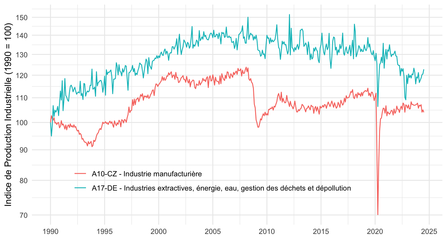
2010-
Code
`IPI-2021` %>%
  filter(NAF2 %in% c("A10-CZ", "A17-DE"),
         CORRECTION == "CVS-CJO",
         NATURE == "INDICE") %>%
  left_join(NAF2, by = "NAF2") %>%
  select_if(function(col) length(unique(col)) > 1) %>%
  month_to_date %>%
  filter(date >= as.Date("2010-01-01")) %>%
  group_by(Naf2) %>%
  mutate(OBS_VALUE = 100*OBS_VALUE/OBS_VALUE[date == as.Date("2010-01-01")]) %>%
  ggplot() + ylab("Indice de Production Industrielle (2010 = 100)") + xlab("") + theme_minimal() +
  geom_line(aes(x = date, y = OBS_VALUE, color = Naf2)) +

  scale_x_date(breaks = seq(1920, 2100, 1) %>% paste0("-01-01") %>% as.Date,
               labels = date_format("%Y")) +
  theme(legend.position = c(0.45, 0.2),
        legend.title = element_blank()) +
  scale_y_log10(breaks = seq(-60, 300, 10))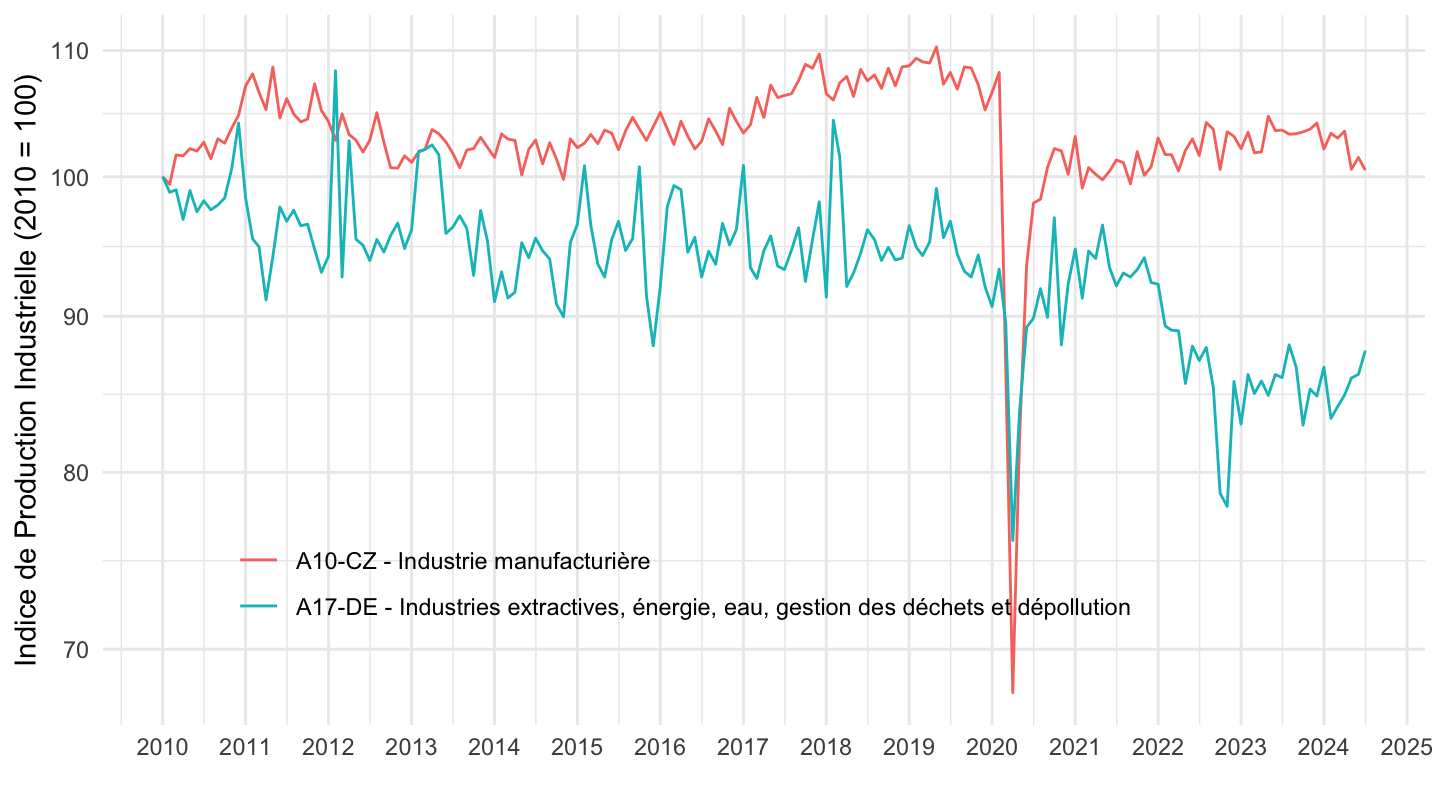
2017-04-
Code
`IPI-2021` %>%
  filter(NAF2 %in% c("A17-DE", "A10-CZ", "A10-BE"),
         CORRECTION == "CVS-CJO",
         NATURE == "INDICE") %>%
  left_join(NAF2, by = "NAF2") %>%
  select_if(function(col) length(unique(col)) > 1) %>%
  month_to_date %>%
  filter(date >= as.Date("2017-04-01")) %>%
  group_by(Naf2) %>%
  mutate(OBS_VALUE = 100*OBS_VALUE/OBS_VALUE[date == as.Date("2020-02-01")]) %>%
  ggplot() + ylab("Indice de Production Industrielle (Février 2020 = 100)") + xlab("") + theme_minimal() +
  geom_line(aes(x = date, y = OBS_VALUE, color = Naf2))  +
  geom_label_repel(data = . %>%
              filter(date == as.Date("2023-12-01")), aes(x = date, y = OBS_VALUE, label = round(OBS_VALUE, 1), color = Naf2), show.legend = F) +
  geom_hline(yintercept = 100, linetype = "dashed") +

  scale_x_date(breaks = seq(1920, 2100, 1) %>% paste0("-01-01") %>% as.Date,
               labels = date_format("%Y")) +
  theme(legend.position = c(0.45, 0.2),
        legend.title = element_blank()) +
  scale_y_log10(breaks = seq(-60, 300, 5))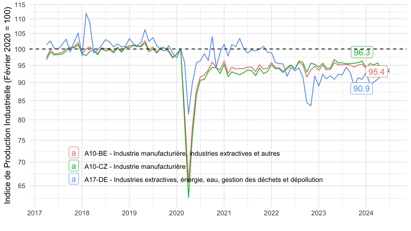
2019-T1
Code
`IPI-2021` %>%
  filter(NAF2 %in% c("A17-DE", "A10-CZ", "A10-BE"),
         CORRECTION == "CVS-CJO",
         NATURE == "INDICE") %>%
  left_join(NAF2, by = "NAF2") %>%
  select_if(function(col) length(unique(col)) > 1) %>%
  month_to_date %>%
  filter(date >= as.Date("2019-01-01")) %>%
  group_by(Naf2) %>%
  mutate(OBS_VALUE = 100*OBS_VALUE/OBS_VALUE[date == as.Date("2019-01-01")]) %>%
  ggplot() + ylab("Indice de Production Industrielle (Janvier 2019 = 100)") + xlab("") + theme_minimal() +
  geom_line(aes(x = date, y = OBS_VALUE, color = Naf2))  +
  geom_label_repel(data = . %>%
              filter(date == max(date)), aes(x = date, y = OBS_VALUE, label = round(OBS_VALUE, 1), color = Naf2), show.legend = F) +
  geom_hline(yintercept = 100, linetype = "dashed") +

  scale_x_date(breaks = seq(1920, 2100, 1) %>% paste0("-01-01") %>% as.Date,
               labels = date_format("%Y")) +
  theme(legend.position = c(0.45, 0.2),
        legend.title = element_blank()) +
  scale_y_log10(breaks = seq(-60, 300, 5))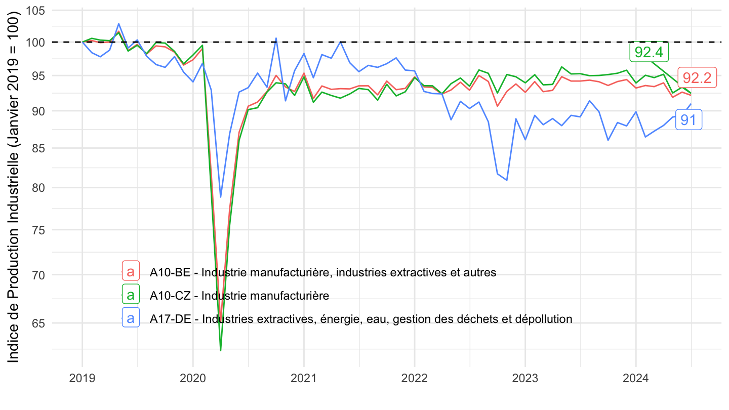
C1, C2, C3
Code
`IPI-2021` %>%
  filter(NAF2 %in% c("A17-C1", "A17-C2", "A17-C3"),
         CORRECTION == "CVS-CJO",
         NATURE == "INDICE") %>%
  left_join(NAF2, by = "NAF2") %>%
  select_if(function(col) length(unique(col)) > 1) %>%
  month_to_date %>%
  group_by(Naf2) %>%
  mutate(OBS_VALUE = 100*OBS_VALUE/OBS_VALUE[date == as.Date("1990-01-01")]) %>%
  ggplot() + ylab("Indice de Production Industrielle") + xlab("") + theme_minimal() +
  geom_line(aes(x = date, y = OBS_VALUE, color = Naf2)) +

  scale_x_date(breaks = seq(1920, 2100, 5) %>% paste0("-01-01") %>% as.Date,
               labels = date_format("%Y")) +
  theme(legend.position = c(0.45, 0.2),
        legend.title = element_blank()) +
  scale_y_log10(breaks = seq(-60, 300, 10))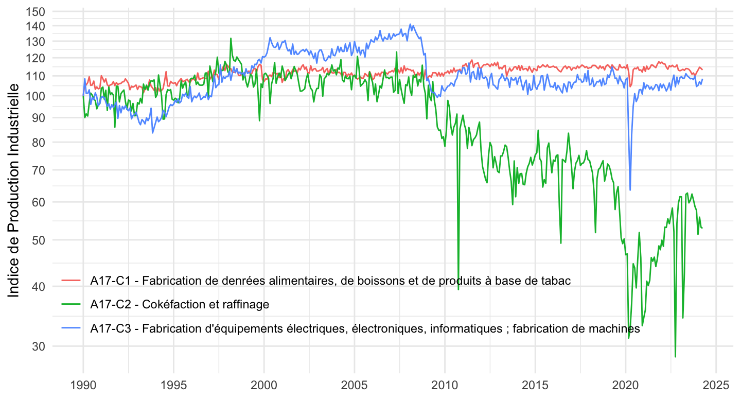
C4, C5
Code
`IPI-2021` %>%
  filter(NAF2 %in% c("A17-C4", "A17-C5"),
         CORRECTION == "CVS-CJO",
         NATURE == "INDICE") %>%
  left_join(NAF2, by = "NAF2") %>%
  select_if(function(col) length(unique(col)) > 1) %>%
  month_to_date %>%
  group_by(Naf2) %>%
  mutate(OBS_VALUE = 100*OBS_VALUE/OBS_VALUE[date == as.Date("1990-01-01")]) %>%
  ggplot() + ylab("Indice de Production Industrielle") + xlab("") + theme_minimal() +
  geom_line(aes(x = date, y = OBS_VALUE, color = Naf2)) +

  scale_x_date(breaks = seq(1920, 2100, 5) %>% paste0("-01-01") %>% as.Date,
               labels = date_format("%Y")) +
  theme(legend.position = c(0.45, 0.2),
        legend.title = element_blank()) +
  scale_y_log10(breaks = seq(-60, 300, 10))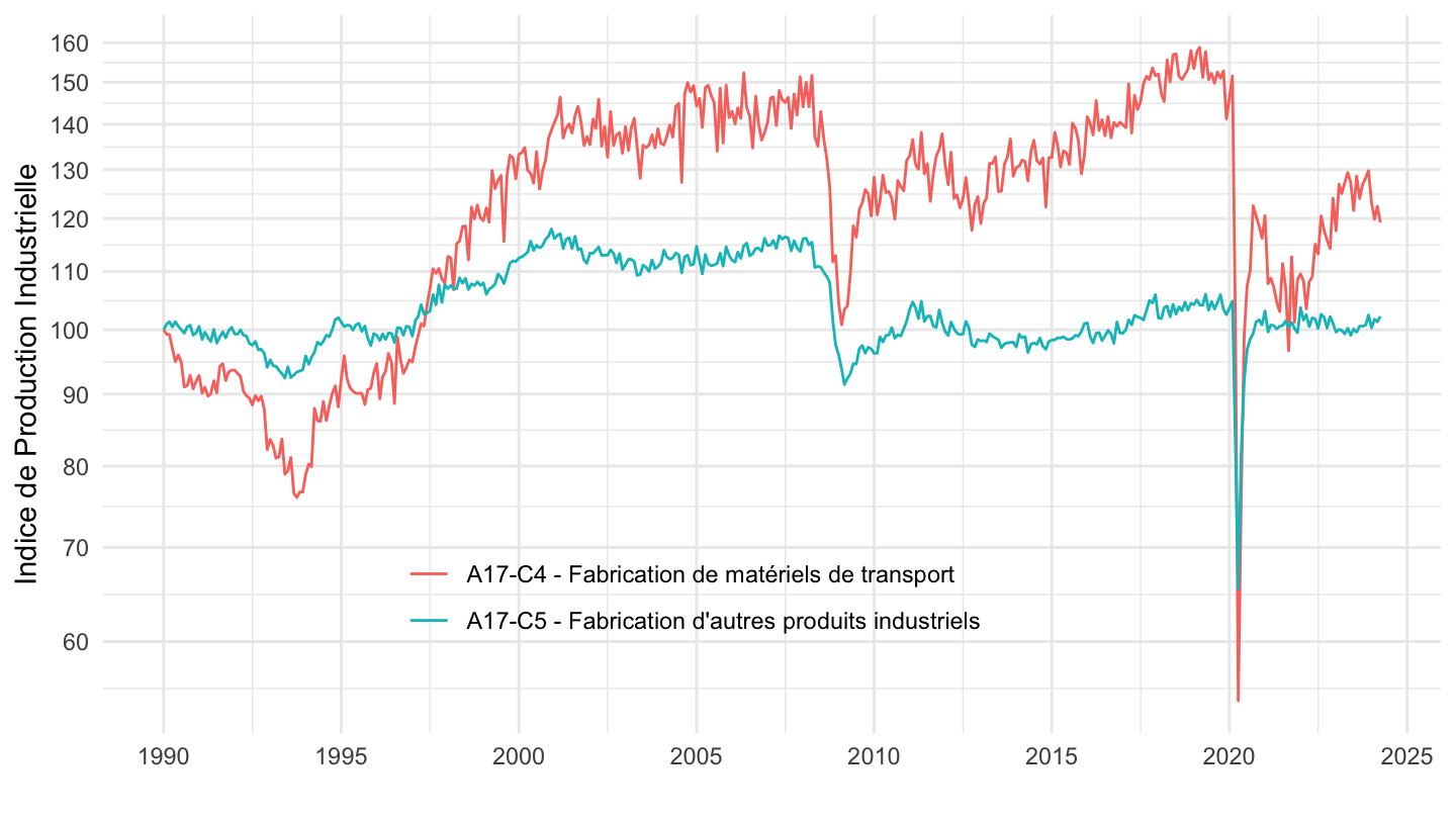
A38
BZ, DZ, EZ
Code
`IPI-2021` %>%
  filter(NAF2 %in% c("A38-BZ", "A38-DZ", "A38-EZ"),
         CORRECTION == "CVS-CJO",
         NATURE == "INDICE") %>%
  left_join(NAF2, by = "NAF2") %>%
  select_if(function(col) length(unique(col)) > 1) %>%
  month_to_date %>%
  group_by(Naf2) %>%
  mutate(OBS_VALUE = 100*OBS_VALUE/OBS_VALUE[date == as.Date("1990-01-01")]) %>%
  ggplot() + ylab("Indice de Production Industrielle") + xlab("") + theme_minimal() +
  geom_line(aes(x = date, y = OBS_VALUE, color = Naf2)) +

  scale_x_date(breaks = seq(1920, 2100, 5) %>% paste0("-01-01") %>% as.Date,
               labels = date_format("%Y")) +
  theme(legend.position = c(0.45, 0.2),
        legend.title = element_blank()) +
  scale_y_log10(breaks = seq(-60, 300, 10))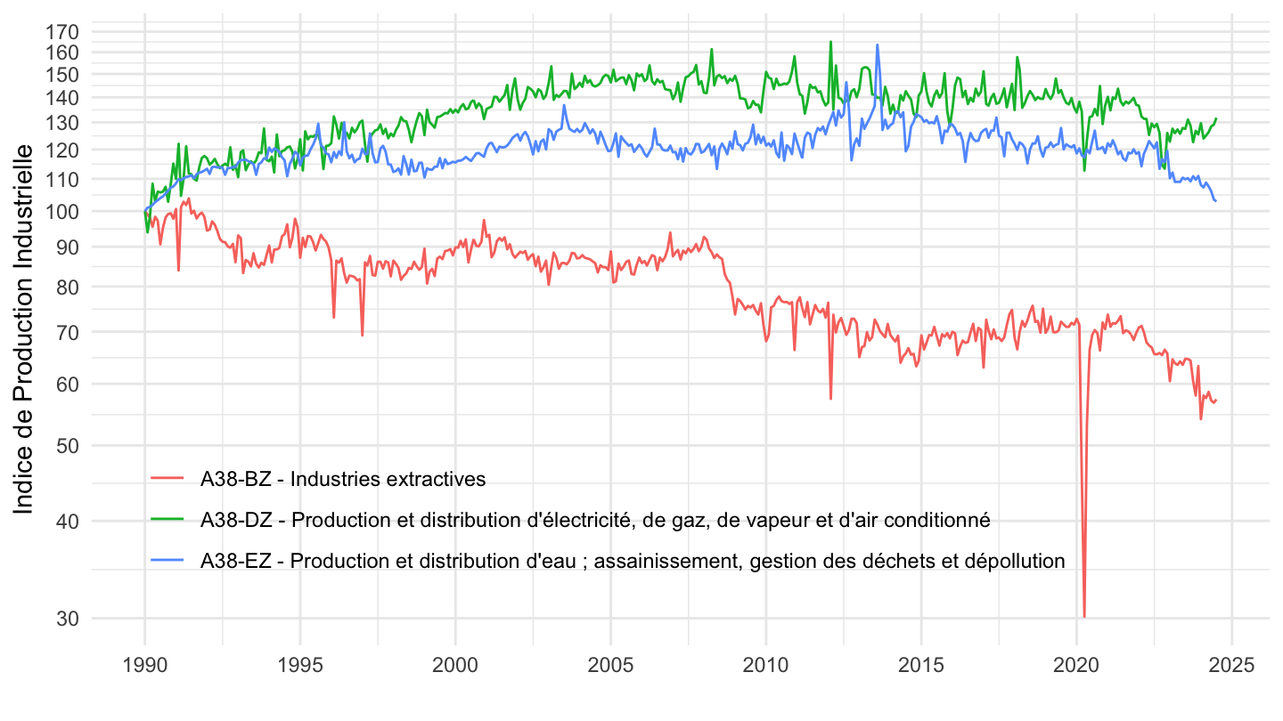
CA, CB, CC
Code
`IPI-2021` %>%
  filter(NAF2 %in% c("A38-CA", "A38-CB", "A38-CC"),
         CORRECTION == "CVS-CJO",
         NATURE == "INDICE") %>%
  left_join(NAF2, by = "NAF2") %>%
  select_if(function(col) length(unique(col)) > 1) %>%
  month_to_date %>%
  group_by(Naf2) %>%
  mutate(OBS_VALUE = 100*OBS_VALUE/OBS_VALUE[date == as.Date("1990-01-01")]) %>%
  ggplot() + ylab("Indice de Production Industrielle") + xlab("") + theme_minimal() +
  geom_line(aes(x = date, y = OBS_VALUE, color = Naf2)) +

  scale_x_date(breaks = seq(1920, 2100, 5) %>% paste0("-01-01") %>% as.Date,
               labels = date_format("%Y")) +
  theme(legend.position = c(0.45, 0.2),
        legend.title = element_blank()) +
  scale_y_log10(breaks = seq(-60, 300, 10))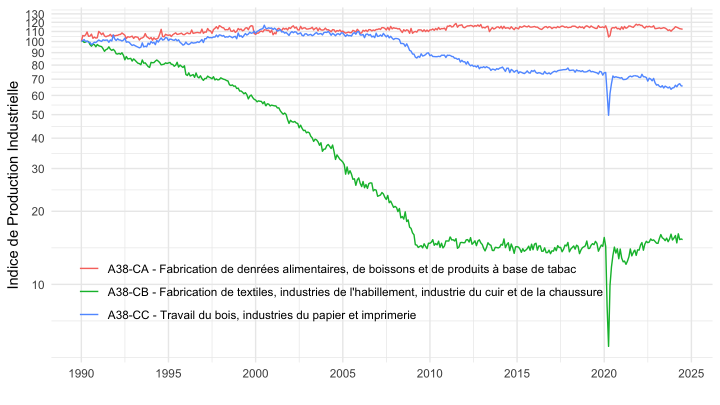
CD, CE, CF
All
Code
`IPI-2021` %>%
  filter(NAF2 %in% c("A38-CD", "A38-CE", "A38-CF"),
         CORRECTION == "CVS-CJO",
         NATURE == "INDICE") %>%
  left_join(NAF2, by = "NAF2") %>%
  select_if(function(col) length(unique(col)) > 1) %>%
  month_to_date %>%
  group_by(Naf2) %>%
  mutate(OBS_VALUE = 100*OBS_VALUE/OBS_VALUE[date == as.Date("1990-01-01")]) %>%
  ggplot() + ylab("Indice de Production Industrielle") + xlab("") + theme_minimal() +
  geom_line(aes(x = date, y = OBS_VALUE, color = Naf2)) +

  scale_x_date(breaks = seq(1920, 2100, 5) %>% paste0("-01-01") %>% as.Date,
               labels = date_format("%Y")) +
  theme(legend.position = c(0.25, 0.2),
        legend.title = element_blank()) +
  scale_y_log10(breaks = seq(-60, 600, 10))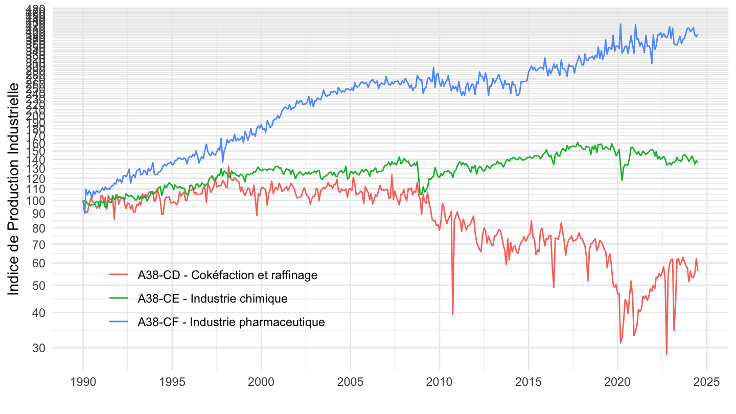
2010-
Code
`IPI-2021` %>%
  filter(NAF2 %in% c("A38-CD", "A38-CE", "A38-CF"),
         CORRECTION == "CVS-CJO",
         NATURE == "INDICE") %>%
  left_join(NAF2, by = "NAF2") %>%
  select_if(function(col) length(unique(col)) > 1) %>%
  month_to_date %>%
  filter(date >= as.Date("2010-01-01")) %>%
  group_by(Naf2) %>%
  mutate(OBS_VALUE = 100*OBS_VALUE/OBS_VALUE[date == as.Date("2010-01-01")]) %>%
  ggplot() + ylab("Indice de Production Industrielle") + xlab("") + theme_minimal() +
  geom_line(aes(x = date, y = OBS_VALUE, color = Naf2)) +

  scale_x_date(breaks = seq(1920, 2100, 1) %>% paste0("-01-01") %>% as.Date,
               labels = date_format("%Y")) +
  theme(legend.position = c(0.25, 0.2),
        legend.title = element_blank()) +
  scale_y_log10(breaks = seq(-60, 600, 10))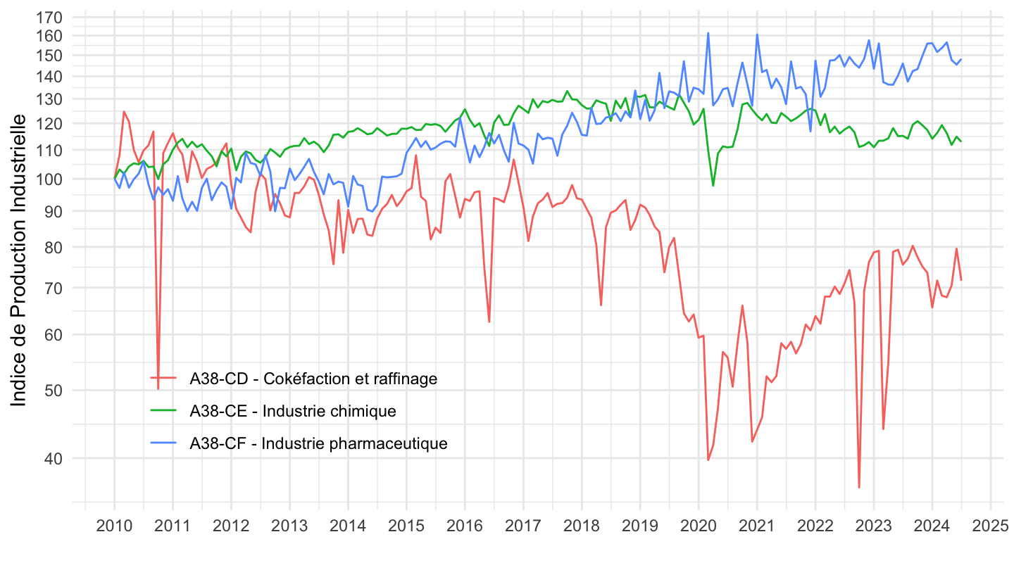
2017-
Code
`IPI-2021` %>%
  filter(NAF2 %in% c("A38-CD", "A38-CE", "A38-CF"),
         CORRECTION == "CVS-CJO",
         NATURE == "INDICE") %>%
  left_join(NAF2, by = "NAF2") %>%
  select_if(function(col) length(unique(col)) > 1) %>%
  month_to_date %>%
  filter(date >= as.Date("2017-01-01")) %>%
  group_by(Naf2) %>%
  mutate(OBS_VALUE = 100*OBS_VALUE/OBS_VALUE[date == as.Date("2017-01-01")]) %>%
  ggplot() + ylab("Indice de Production Industrielle") + xlab("") + theme_minimal() +
  geom_line(aes(x = date, y = OBS_VALUE, color = Naf2)) +

  scale_x_date(breaks = seq(1920, 2100, 1) %>% paste0("-01-01") %>% as.Date,
               labels = date_format("%Y")) +
  theme(legend.position = c(0.25, 0.2),
        legend.title = element_blank()) +
  scale_y_log10(breaks = seq(-60, 600, 10))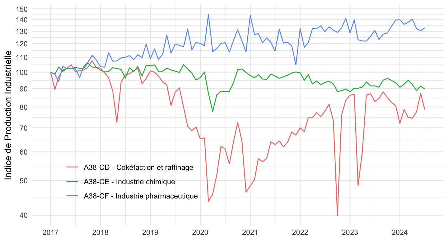
CG, CH, CI
All
Code
`IPI-2021` %>%
  filter(NAF2 %in% c("A38-CG", "A38-CH", "A38-CI"),
         CORRECTION == "CVS-CJO",
         NATURE == "INDICE") %>%
  left_join(NAF2, by = "NAF2") %>%
  select_if(function(col) length(unique(col)) > 1) %>%
  month_to_date %>%
  group_by(Naf2) %>%
  mutate(OBS_VALUE = 100*OBS_VALUE/OBS_VALUE[date == as.Date("1990-01-01")]) %>%
  ggplot() + ylab("Indice de Production Industrielle") + xlab("") + theme_minimal() +
  geom_line(aes(x = date, y = OBS_VALUE, color = Naf2)) +

  scale_x_date(breaks = seq(1920, 2100, 5) %>% paste0("-01-01") %>% as.Date,
               labels = date_format("%Y")) +
  theme(legend.position = c(0.5, 0.2),
        legend.title = element_blank()) +
  scale_y_log10(breaks = seq(-60, 300, 10))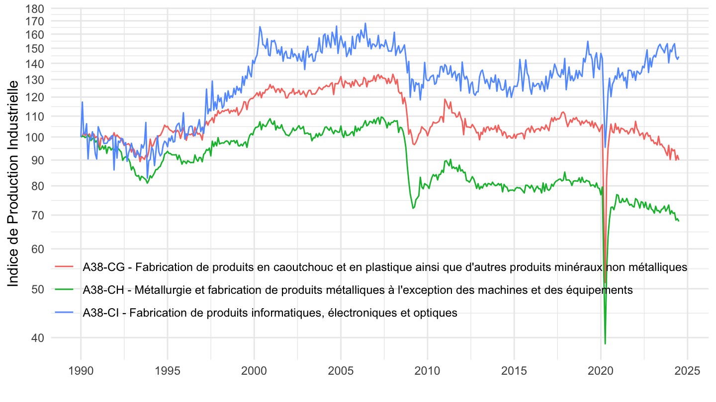
2017-
Code
`IPI-2021` %>%
  filter(NAF2 %in% c("A38-CG", "A38-CH", "A38-CI"),
         CORRECTION == "CVS-CJO",
         NATURE == "INDICE") %>%
  left_join(NAF2, by = "NAF2") %>%
  select_if(function(col) length(unique(col)) > 1) %>%
  month_to_date %>%
  filter(date >= as.Date("2017-01-01")) %>%
  group_by(Naf2) %>%
  mutate(OBS_VALUE = 100*OBS_VALUE/OBS_VALUE[date == as.Date("2017-01-01")]) %>%
  ggplot() + ylab("Indice de Production Industrielle") + xlab("") + theme_minimal() +
  geom_line(aes(x = date, y = OBS_VALUE, color = Naf2)) +

  scale_x_date(breaks = seq(1920, 2100, 1) %>% paste0("-01-01") %>% as.Date,
               labels = date_format("%Y")) +
  theme(legend.position = c(0.5, 0.2),
        legend.title = element_blank()) +
  scale_y_log10(breaks = seq(-60, 300, 10))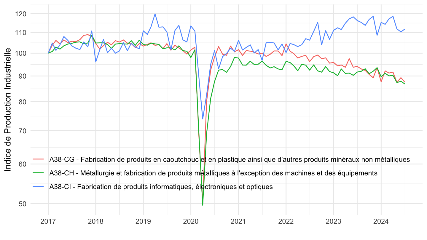
CJ, CK, CM
Code
`IPI-2021` %>%
  filter(NAF2 %in% c("A38-CJ", "A38-CK", "A38-CM"),
         CORRECTION == "CVS-CJO",
         NATURE == "INDICE") %>%
  left_join(NAF2, by = "NAF2") %>%
  select_if(function(col) length(unique(col)) > 1) %>%
  month_to_date %>%
  group_by(Naf2) %>%
  mutate(OBS_VALUE = 100*OBS_VALUE/OBS_VALUE[date == as.Date("1990-01-01")]) %>%
  ggplot() + ylab("Indice de Production Industrielle") + xlab("") + theme_minimal() +
  geom_line(aes(x = date, y = OBS_VALUE, color = Naf2)) +

  scale_x_date(breaks = seq(1920, 2100, 5) %>% paste0("-01-01") %>% as.Date,
               labels = date_format("%Y")) +
  theme(legend.position = c(0.5, 0.2),
        legend.title = element_blank()) +
  scale_y_log10(breaks = seq(-60, 300, 10))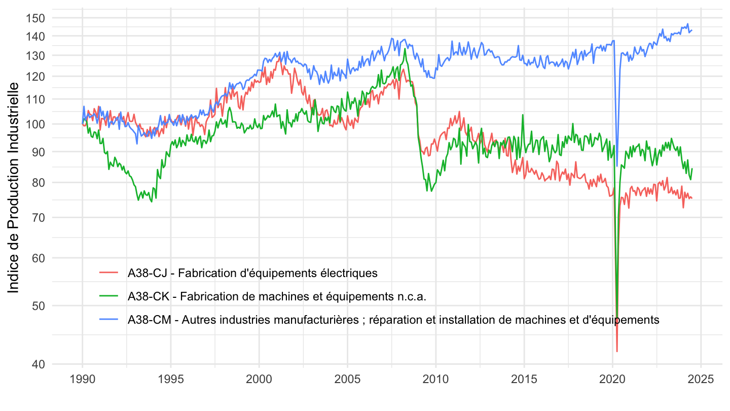
CL, CL1, CL2
Code
`IPI-2021` %>%
  filter(NAF2 %in% c("A38-CL", "CL1", "CL2"),
         CORRECTION == "CVS-CJO",
         NATURE == "INDICE") %>%
  left_join(NAF2, by = "NAF2") %>%
  select_if(function(col) length(unique(col)) > 1) %>%
  month_to_date %>%
  group_by(Naf2) %>%
  mutate(OBS_VALUE = 100*OBS_VALUE/OBS_VALUE[date == as.Date("1990-01-01")]) %>%
  ggplot() + ylab("Indice de Production Industrielle") + xlab("") + theme_minimal() +
  geom_line(aes(x = date, y = OBS_VALUE, color = Naf2)) +

  scale_x_date(breaks = seq(1920, 2100, 5) %>% paste0("-01-01") %>% as.Date,
               labels = date_format("%Y")) +
  theme(legend.position = c(0.5, 0.2),
        legend.title = element_blank()) +
  scale_y_log10(breaks = seq(-60, 300, 10))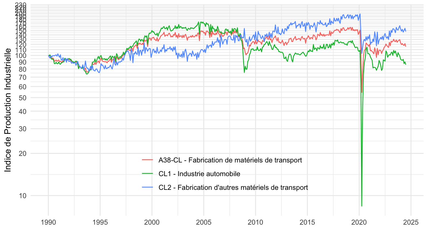
A88 (2-digit NAF)
06, 08
Code
`IPI-2021` %>%
  filter(NAF2 %in% c("06", "08"),
         CORRECTION == "CVS-CJO",
         NATURE == "INDICE") %>%
  left_join(NAF2, by = "NAF2") %>%
  select_if(function(col) length(unique(col)) > 1) %>%
  month_to_date %>%
  group_by(Naf2) %>%
  mutate(OBS_VALUE = 100*OBS_VALUE/OBS_VALUE[date == as.Date("1990-01-01")]) %>%
  ggplot() + ylab("Indice de Production Industrielle") + xlab("") + theme_minimal() +
  geom_line(aes(x = date, y = OBS_VALUE, color = Naf2)) +

  scale_x_date(breaks = seq(1920, 2100, 5) %>% paste0("-01-01") %>% as.Date,
               labels = date_format("%Y")) +
  theme(legend.position = c(0.5, 0.2),
        legend.title = element_blank()) +
  scale_y_log10(breaks = seq(-60, 300, 10))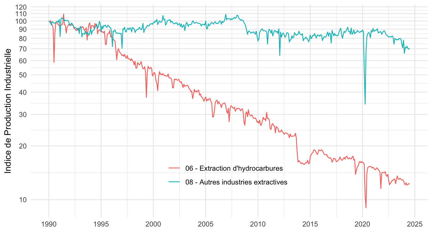
10, 11
Code
`IPI-2021` %>%
  filter(NAF2 %in% c("10", "11"),
         CORRECTION == "CVS-CJO",
         NATURE == "INDICE") %>%
  left_join(NAF2, by = "NAF2") %>%
  select_if(function(col) length(unique(col)) > 1) %>%
  month_to_date %>%
  group_by(Naf2) %>%
  mutate(OBS_VALUE = 100*OBS_VALUE/OBS_VALUE[date == as.Date("1990-01-01")]) %>%
  ggplot() + ylab("Indice de Production Industrielle") + xlab("") + theme_minimal() +
  geom_line(aes(x = date, y = OBS_VALUE, color = Naf2)) +

  scale_x_date(breaks = seq(1920, 2100, 5) %>% paste0("-01-01") %>% as.Date,
               labels = date_format("%Y")) +
  theme(legend.position = c(0.5, 0.2),
        legend.title = element_blank()) +
  scale_y_log10(breaks = seq(-60, 300, 10))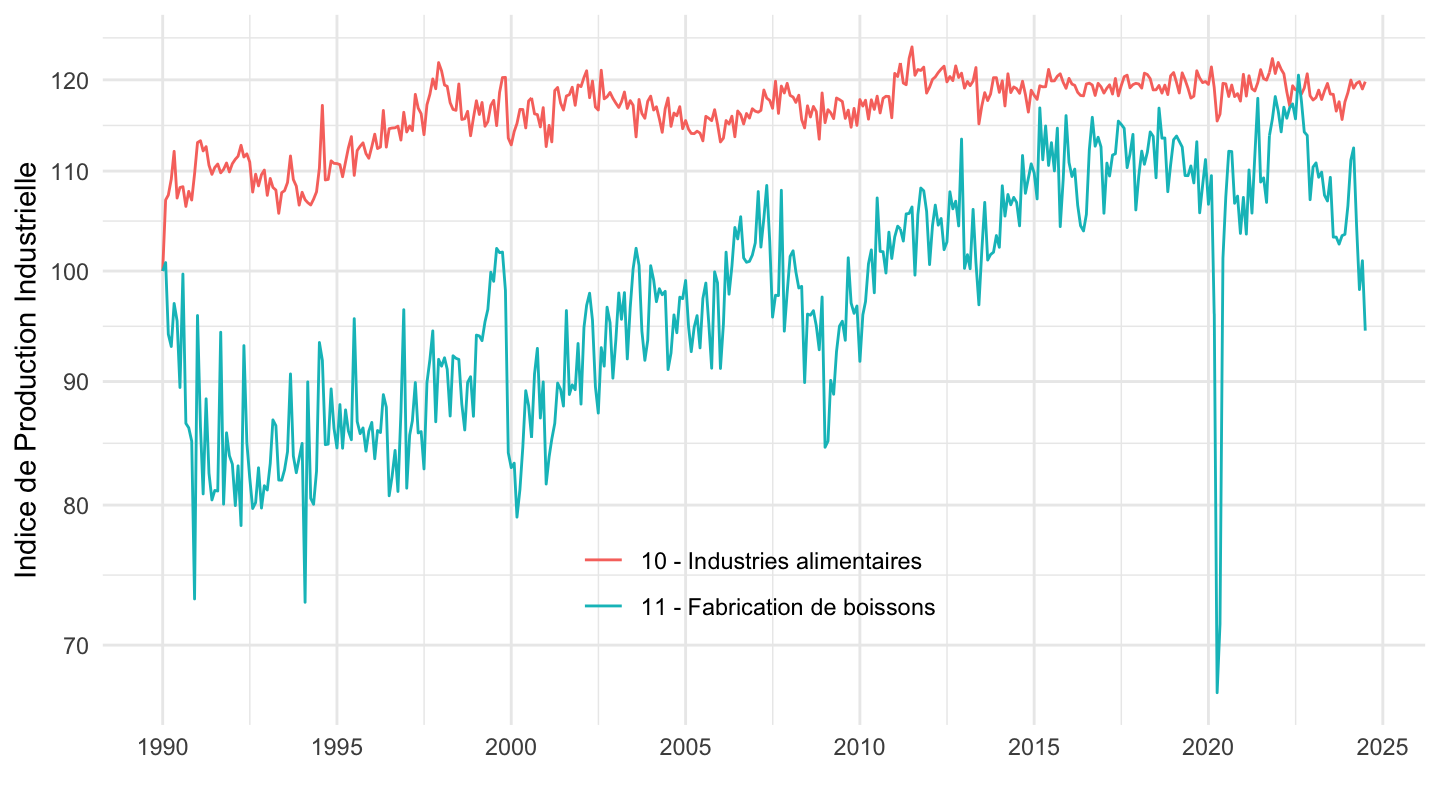
10, 11, 12
Code
`IPI-2021` %>%
  filter(NAF2 %in% c("10", "11", "12"),
         CORRECTION == "CVS-CJO",
         NATURE == "INDICE") %>%
  left_join(NAF2, by = "NAF2") %>%
  select_if(function(col) length(unique(col)) > 1) %>%
  month_to_date %>%
  group_by(Naf2) %>%
  mutate(OBS_VALUE = 100*OBS_VALUE/OBS_VALUE[date == as.Date("1990-01-01")]) %>%
  ggplot() + ylab("Indice de Production Industrielle") + xlab("") + theme_minimal() +
  geom_line(aes(x = date, y = OBS_VALUE, color = Naf2)) +

  scale_x_date(breaks = seq(1920, 2100, 5) %>% paste0("-01-01") %>% as.Date,
               labels = date_format("%Y")) +
  theme(legend.position = c(0.5, 0.2),
        legend.title = element_blank()) +
  scale_y_log10(breaks = seq(-60, 300, 10))
13, 14, 15
Code
`IPI-2021` %>%
  filter(NAF2 %in% c("13", "14", "15"),
         CORRECTION == "CVS-CJO",
         NATURE == "INDICE") %>%
  left_join(NAF2, by = "NAF2") %>%
  select_if(function(col) length(unique(col)) > 1) %>%
  month_to_date %>%
  group_by(Naf2) %>%
  mutate(OBS_VALUE = 100*OBS_VALUE/OBS_VALUE[date == as.Date("1990-01-01")]) %>%
  ggplot() + ylab("Indice de Production Industrielle") + xlab("") + theme_minimal() +
  geom_line(aes(x = date, y = OBS_VALUE, color = Naf2)) +

  scale_x_date(breaks = seq(1920, 2100, 5) %>% paste0("-01-01") %>% as.Date,
               labels = date_format("%Y")) +
  theme(legend.position = c(0.3, 0.2),
        legend.title = element_blank()) +
  scale_y_log10(breaks = seq(-60, 300, 10))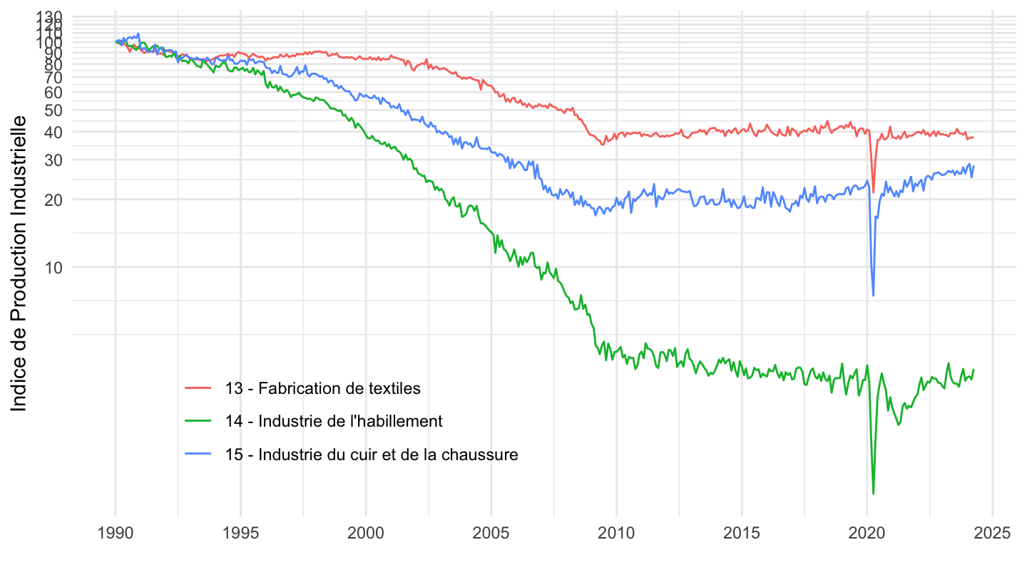
16, 17, 18
Code
`IPI-2021` %>%
  filter(NAF2 %in% c("16", "17", "18"),
         CORRECTION == "CVS-CJO",
         NATURE == "INDICE") %>%
  left_join(NAF2, by = "NAF2") %>%
  select_if(function(col) length(unique(col)) > 1) %>%
  month_to_date %>%
  group_by(Naf2) %>%
  mutate(OBS_VALUE = 100*OBS_VALUE/OBS_VALUE[date == as.Date("1990-01-01")]) %>%
  ggplot() + ylab("Indice de Production Industrielle") + xlab("") + theme_minimal() +
  geom_line(aes(x = date, y = OBS_VALUE, color = Naf2)) +

  scale_x_date(breaks = seq(1920, 2100, 5) %>% paste0("-01-01") %>% as.Date,
               labels = date_format("%Y")) +
  theme(legend.position = c(0.6, 0.2),
        legend.title = element_blank()) +
  scale_y_log10(breaks = seq(-60, 300, 10))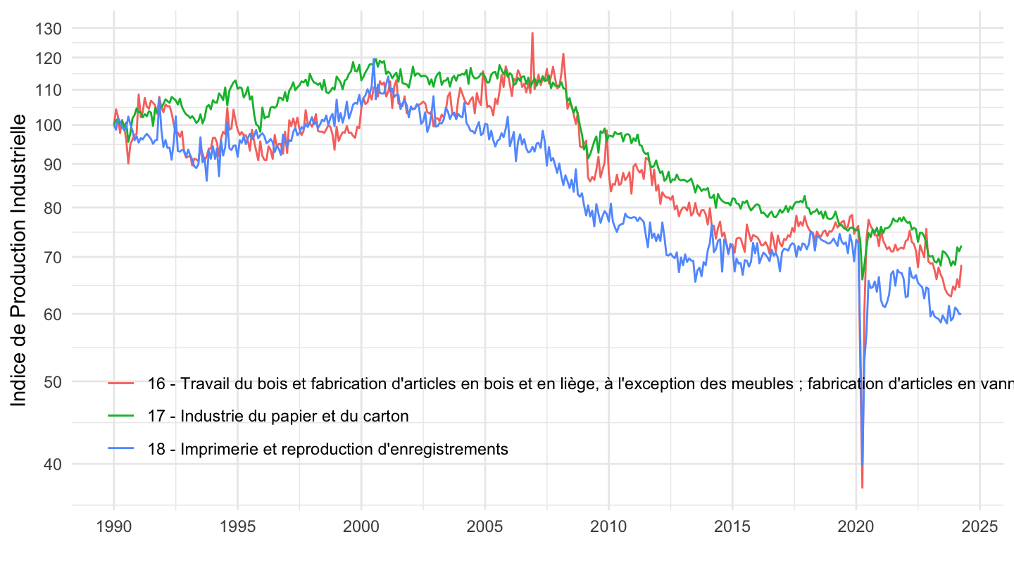
19, 20, 21
Code
`IPI-2021` %>%
  filter(NAF2 %in% c("19", "20", "21"),
         CORRECTION == "CVS-CJO",
         NATURE == "INDICE") %>%
  left_join(NAF2, by = "NAF2") %>%
  select_if(function(col) length(unique(col)) > 1) %>%
  month_to_date %>%
  group_by(Naf2) %>%
  mutate(OBS_VALUE = 100*OBS_VALUE/OBS_VALUE[date == as.Date("1990-01-01")]) %>%
  ggplot() + ylab("Indice de Production Industrielle") + xlab("") + theme_minimal() +
  geom_line(aes(x = date, y = OBS_VALUE, color = Naf2)) +

  scale_x_date(breaks = seq(1920, 2100, 5) %>% paste0("-01-01") %>% as.Date,
               labels = date_format("%Y")) +
  theme(legend.position = c(0.3, 0.2),
        legend.title = element_blank()) +
  scale_y_log10(breaks = seq(0, 600, 50))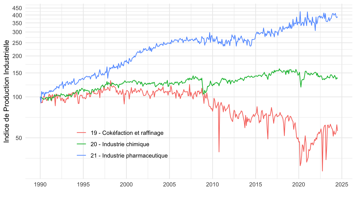
22, 23, 24
Code
`IPI-2021` %>%
  filter(NAF2 %in% c("22", "23", "24"),
         CORRECTION == "CVS-CJO",
         NATURE == "INDICE") %>%
  left_join(NAF2, by = "NAF2") %>%
  select_if(function(col) length(unique(col)) > 1) %>%
  month_to_date %>%
  group_by(Naf2) %>%
  mutate(OBS_VALUE = 100*OBS_VALUE/OBS_VALUE[date == as.Date("1990-01-01")]) %>%
  ggplot() + ylab("Indice de Production Industrielle") + xlab("") + theme_minimal() +
  geom_line(aes(x = date, y = OBS_VALUE, color = Naf2)) +

  scale_x_date(breaks = seq(1920, 2100, 5) %>% paste0("-01-01") %>% as.Date,
               labels = date_format("%Y")) +
  theme(legend.position = c(0.3, 0.2),
        legend.title = element_blank()) +
  scale_y_log10(breaks = seq(0, 600, 10))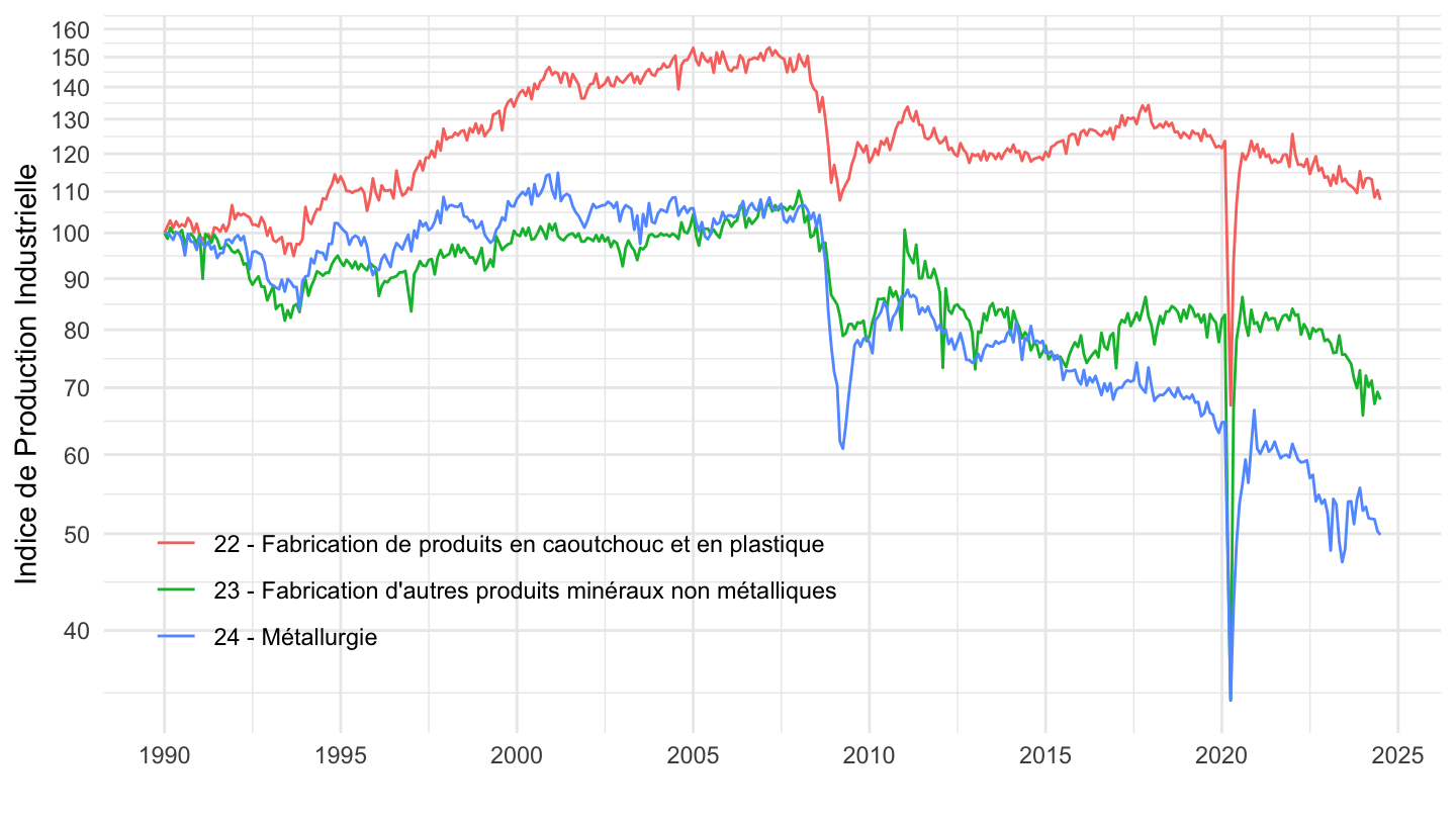
25, 26, 27
Code
`IPI-2021` %>%
  filter(NAF2 %in% c("22", "26", "27"),
         CORRECTION == "CVS-CJO",
         NATURE == "INDICE") %>%
  left_join(NAF2, by = "NAF2") %>%
  select_if(function(col) length(unique(col)) > 1) %>%
  month_to_date %>%
  group_by(Naf2) %>%
  mutate(OBS_VALUE = 100*OBS_VALUE/OBS_VALUE[date == as.Date("1990-01-01")]) %>%
  ggplot() + ylab("Indice de Production Industrielle") + xlab("") + theme_minimal() +
  geom_line(aes(x = date, y = OBS_VALUE, color = Naf2)) +

  scale_x_date(breaks = seq(1920, 2100, 5) %>% paste0("-01-01") %>% as.Date,
               labels = date_format("%Y")) +
  theme(legend.position = c(0.4, 0.2),
        legend.title = element_blank()) +
  scale_y_log10(breaks = seq(0, 600, 10))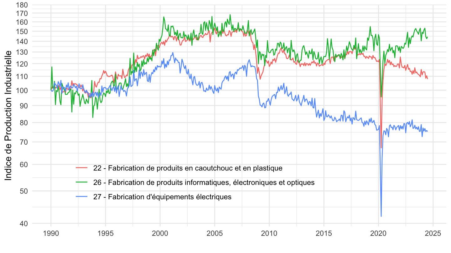
28, 29, 30
Code
`IPI-2021` %>%
  filter(NAF2 %in% c("28", "29", "30"),
         CORRECTION == "CVS-CJO",
         NATURE == "INDICE") %>%
  left_join(NAF2, by = "NAF2") %>%
  select_if(function(col) length(unique(col)) > 1) %>%
  month_to_date %>%
  group_by(Naf2) %>%
  mutate(OBS_VALUE = 100*OBS_VALUE/OBS_VALUE[date == as.Date("1990-01-01")]) %>%
  ggplot() + ylab("Indice de Production Industrielle") + xlab("") + theme_minimal() +
  geom_line(aes(x = date, y = OBS_VALUE, color = Naf2)) +

  scale_x_date(breaks = seq(1920, 2100, 5) %>% paste0("-01-01") %>% as.Date,
               labels = date_format("%Y")) +
  theme(legend.position = c(0.4, 0.2),
        legend.title = element_blank()) +
  scale_y_log10(breaks = seq(0, 600, 10))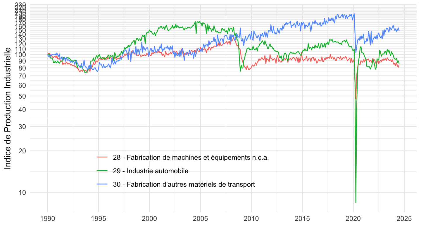
31, 32, 33
Code
`IPI-2021` %>%
  filter(NAF2 %in% c("31", "32", "33"),
         CORRECTION == "CVS-CJO",
         NATURE == "INDICE") %>%
  left_join(NAF2, by = "NAF2") %>%
  select_if(function(col) length(unique(col)) > 1) %>%
  month_to_date %>%
  group_by(Naf2) %>%
  mutate(OBS_VALUE = 100*OBS_VALUE/OBS_VALUE[date == as.Date("1990-01-01")]) %>%
  ggplot() + ylab("Indice de Production Industrielle") + xlab("") + theme_minimal() +
  geom_line(aes(x = date, y = OBS_VALUE, color = Naf2)) +

  scale_x_date(breaks = seq(1920, 2100, 5) %>% paste0("-01-01") %>% as.Date,
               labels = date_format("%Y")) +
  theme(legend.position = c(0.4, 0.2),
        legend.title = element_blank()) +
  scale_y_log10(breaks = seq(0, 600, 10))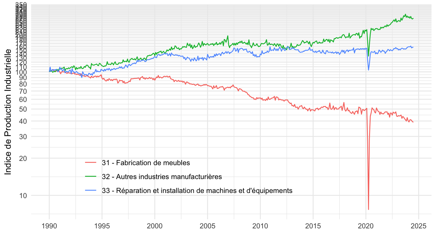
35, 36
Code
`IPI-2021` %>%
  filter(NAF2 %in% c("35", "36"),
         CORRECTION == "CVS-CJO",
         NATURE == "INDICE") %>%
  left_join(NAF2, by = "NAF2") %>%
  select_if(function(col) length(unique(col)) > 1) %>%
  month_to_date %>%
  group_by(Naf2) %>%
  mutate(OBS_VALUE = 100*OBS_VALUE/OBS_VALUE[date == as.Date("1990-01-01")]) %>%
  ggplot() + ylab("Indice de Production Industrielle") + xlab("") + theme_minimal() +
  geom_line(aes(x = date, y = OBS_VALUE, color = Naf2)) +

  scale_x_date(breaks = seq(1920, 2100, 5) %>% paste0("-01-01") %>% as.Date,
               labels = date_format("%Y")) +
  theme(legend.position = c(0.6, 0.2),
        legend.title = element_blank()) +
  scale_y_log10(breaks = seq(0, 600, 10))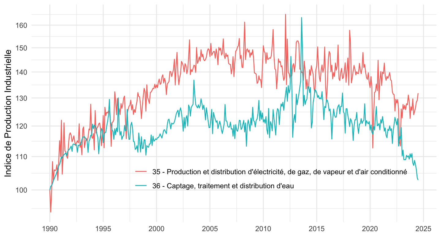
Electricité
Tous les postes
Code
`IPI-2021` %>%
  filter(NAF2 %in% c("35", "35-11", "A10-BE", "A17-DE", "A38-DZ"),
         CORRECTION == "CVS-CJO",
         NATURE == "INDICE") %>%
  left_join(NAF2, by = "NAF2") %>%
  select_if(function(col) length(unique(col)) > 1) %>%
  month_to_date %>%
  group_by(Naf2) %>%
  mutate(OBS_VALUE = 100*OBS_VALUE/OBS_VALUE[date == as.Date("1990-01-01")]) %>%
  ggplot() + ylab("Indice de Production Industrielle") + xlab("") + theme_minimal() +
  geom_line(aes(x = date, y = OBS_VALUE, color = Naf2)) +

  scale_x_date(breaks = seq(1920, 2100, 5) %>% paste0("-01-01") %>% as.Date,
               labels = date_format("%Y")) +
  theme(legend.position = c(0.6, 0.2),
        legend.title = element_blank()) +
  scale_y_log10(breaks = seq(0, 600, 10))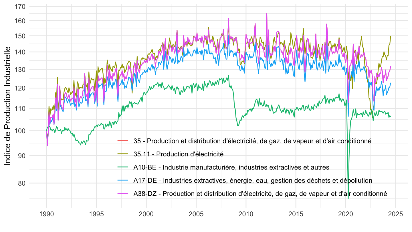
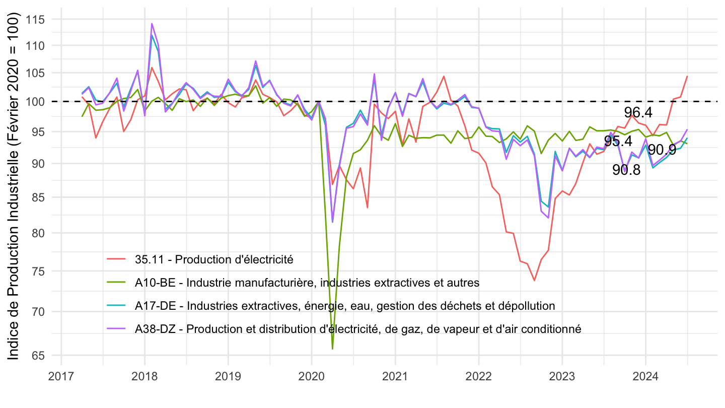
2017-04-
Code
`IPI-2021` %>%
  filter(NAF2 %in% c("35-11", "A10-BE", "A17-DE", "A38-DZ"),
         CORRECTION == "CVS-CJO",
         NATURE == "INDICE") %>%
  left_join(NAF2, by = "NAF2") %>%
  select_if(function(col) length(unique(col)) > 1) %>%
  month_to_date %>%
  filter(date >= as.Date("2017-04-01")) %>%
  group_by(Naf2) %>%
  mutate(OBS_VALUE = 100*OBS_VALUE/OBS_VALUE[date == as.Date("2020-02-01")]) %>%
  ggplot() + ylab("Indice de Production Industrielle (Février 2020 = 100)") + xlab("") + theme_minimal() +
  geom_line(aes(x = date, y = OBS_VALUE, color = Naf2))  +
  geom_text_repel(data = . %>%
              filter(date == as.Date("2023-12-01")), aes(x = date, y = OBS_VALUE, label = round(OBS_VALUE, 1))) +
  geom_hline(yintercept = 100, linetype = "dashed") +

  scale_x_date(breaks = seq(1920, 2100, 1) %>% paste0("-01-01") %>% as.Date,
               labels = date_format("%Y")) +
  theme(legend.position = c(0.45, 0.2),
        legend.title = element_blank()) +
  scale_y_log10(breaks = seq(-60, 300, 5))