| source | dataset | Title | .html | .rData |
|---|---|---|---|---|
| oecd | HOU_EAR | Hourly Earnings | 2026-07-24 | 2026-07-24 |
| oecd | PRICES_CPI | Consumer price indices (CPIs) | 2024-04-16 | 2024-04-15 |
Hourly Earnings
Data - OECD
Info
Data on wages
Code
load_data("wages.RData")
wages %>%
source_dataset_title_file_updates()| Title | source | dataset | .html | .RData |
|---|---|---|---|---|
| Monthly minimum wages - bi-annual data | eurostat | earn_mw_cur | 2026-07-23 | 2026-04-14 |
| Labour cost index, nominal value - quarterly data | eurostat | ei_lmlc_q | 2026-07-23 | NA |
| Labour cost levels by NACE Rev. 2 activity | eurostat | lc_lci_lev | 2026-07-24 | 2026-04-14 |
| Labour cost index by NACE Rev. 2 activity - nominal value, quarterly data | eurostat | lc_lci_r2_q | 2026-07-24 | NA |
| Labour productivity and unit labour costs | eurostat | nama_10_lp_ulc | 2026-07-22 | 2026-04-14 |
| Labour productivity and unit labour costs | eurostat | namq_10_lp_ulc | 2026-07-24 | NA |
| Minimum wages | eurostat | tps00155 | 2026-07-24 | NA |
| Wage | fred | wage | 2026-07-25 | 2026-07-24 |
| Mean nominal monthly earnings of employees by sex and economic activity -- Harmonized series | ilo | EAR_4MTH_SEX_ECO_CUR_NB_A | 2026-07-25 | 2023-06-01 |
| Mean nominal monthly earnings of employees by sex and economic activity -- Harmonized series | ilo | EAR_XEES_SEX_ECO_NB_Q | 2026-07-25 | 2023-06-01 |
| Average annual wages | oecd | AV_AN_WAGE | 2026-07-26 | 2026-04-14 |
| Taxing Wages - Comparative tables | oecd | AWCOMP | 2026-07-26 | 2023-09-09 |
| Hourly Earnings (MEI) | oecd | EAR_MEI | 2026-07-26 | 2024-04-16 |
| Household Dashboard | oecd | HH_DASH | 2026-07-26 | 2023-09-09 |
| Minimum relative to average wages of full-time workers - MIN2AVE | oecd | MIN2AVE | 2026-02-22 | 2023-09-09 |
| Real Minimum Wages - RMW | oecd | RMW | 2026-07-24 | 2024-03-12 |
| Unit labour costs and labour productivity (employment based), Total economy | oecd | ULC_EEQ | 2026-07-24 | 2024-04-15 |
Last
| obsTime | FREQ | Nobs |
|---|---|---|
| 2025 | A | 6 |
| 2024 | A | 92 |
| 2023 | A | 95 |
| 2026-03 | M | 3 |
| 2026-02 | M | 3 |
| 2026-01 | M | 3 |
| 2026-Q1 | Q | 3 |
| 2025-Q4 | Q | 6 |
| 2025-Q3 | Q | 62 |
Detail
The Hourly Earnings dataset contains predominantly monthly statistics, and associated statistical methodological information, for the OECD member countries and for selected non-member economies.
The Hourly Earnings dataset provides monthly and quarterly data on employees’ earnings series. It includes earnings series in manufacturing and for the private economic sector. Mostly the sources of the data are business surveys covering different economic sectors, but in some cases administrative data are also used.
The target series for hourly earnings correspond to seasonally adjusted average total earnings paid per employed person per hour, including overtime pay and regularly recurring cash supplements. Where hourly earnings series are not available, a series could refer to weekly or monthly earnings. In this case, a series for full-time or full-time equivalent employees is preferred to an all employees series.
SECTOR
Code
HOU_EAR %>%
  group_by(SECTOR, `Institutional sector`) %>%
  summarise(nobs = n()) %>%
  arrange(-nobs) %>%
print_table_conditional()| SECTOR | Institutional sector | nobs |
|---|---|---|
| S1 | Total economy | 32038 |
| S1D | Private sector | 7431 |
ADJUSTMENT
Code
HOU_EAR %>%
  group_by(ADJUSTMENT, Adjustment) %>%
  summarise(nobs = n()) %>%
  arrange(-nobs) %>%
print_table_conditional()| ADJUSTMENT | Adjustment | nobs |
|---|---|---|
| Y | Calendar and seasonally adjusted | 23894 |
| N | Neither seasonally adjusted nor calendar adjusted | 15575 |
FREQ
Code
HOU_EAR %>%
  group_by(FREQ, `Frequency of observation`) %>%
  summarise(nobs = n()) %>%
  arrange(-nobs) %>%
print_table_conditional()| FREQ | Frequency of observation | nobs |
|---|---|---|
| M | Monthly | 20904 |
| Q | Quarterly | 14785 |
| A | Annual | 3780 |
REF_AREA
Code
HOU_EAR %>%
  group_by(REF_AREA, Ref_area) %>%
  summarise(Nobs = n()) %>%
  mutate(Flag = gsub(" ", "-", str_to_lower(gsub(" ", "-", Ref_area))),
         Flag = paste0('<img src="../../icon/flag/vsmall/', Flag, '.png" alt="Flag">')) %>%
  select(Flag, everything()) %>%
  {if (is_html_output()) datatable(., filter = 'top', rownames = F, escape = F) else .}
obsTime
Code
HOU_EAR %>%
  group_by(obsTime) %>%
  summarise(Nobs = n()) %>%
  arrange(desc(obsTime)) %>%
  print_table_conditional()
Eurozone, United States
All
Code
HOU_EAR %>%
  filter(SECTOR == "S1",
         FREQ == "Q",
         REF_AREA %in% c("USA", "EA19"),
         ADJUSTMENT == "Y") %>%
  quarter_to_date %>%
  mutate(Ref_area = ifelse(REF_AREA == "EA19", "Europe", Ref_area)) %>%
  left_join(colors, by = c("Ref_area" = "country")) %>%
  mutate(color = ifelse(REF_AREA == "EA19", color2, color)) %>%
  rename(Location = Ref_area) %>%
  ggplot(.) + geom_line(aes(x = date, y = obsValue, color = color)) +
  scale_color_identity() + theme_minimal() + add_2flags +
  scale_x_date(breaks = seq(1920, 2100, 5) %>% paste0("-01-01") %>% as.Date,
               labels = date_format("%Y")) +
  scale_y_log10(breaks = seq(10, 500, 10),
                     labels = scales::dollar_format(accuracy = 1, suffix = "", prefix = "")) +
  ylab("") + xlab("")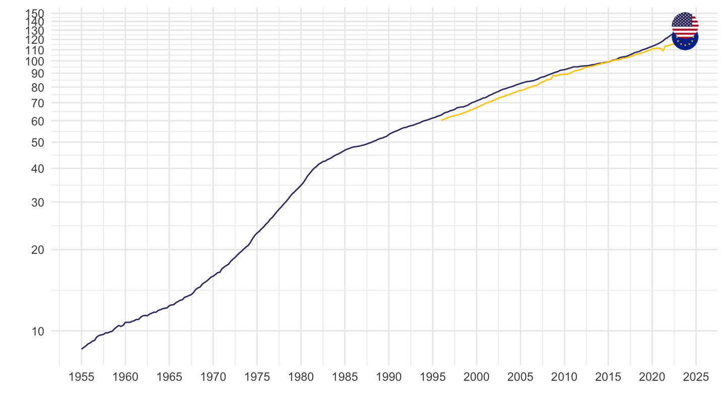
1996-
Quarterly
Code
HOU_EAR %>%
  filter(SECTOR == "S1",
         FREQ == "Q",
         REF_AREA %in% c("USA", "EA19"),
         ADJUSTMENT == "Y") %>%
  quarter_to_date %>%
  filter(date >= as.Date("1996-01-01")) %>%

  group_by(REF_AREA) %>%
  arrange(date) %>%
  mutate(obsValue = 100*obsValue/obsValue[1]) %>%
  mutate(Ref_area = ifelse(REF_AREA == "EA19", "Europe", Ref_area)) %>%
  left_join(colors, by = c("Ref_area" = "country")) %>%
  mutate(color = ifelse(REF_AREA == "EA19", color2, color)) %>%
  rename(Location = Ref_area) %>%
  ggplot(.) + geom_line(aes(x = date, y = obsValue, color = color)) +
  scale_color_identity() + theme_minimal() + add_2flags +
  scale_x_date(breaks = seq(1996, 2100, 2) %>% paste0("-01-01") %>% as.Date,
               labels = date_format("%Y")) +
  scale_y_log10(breaks = seq(10, 500, 10),
                     labels = scales::dollar_format(accuracy = 1, suffix = "", prefix = "")) +
  ylab("") + xlab("")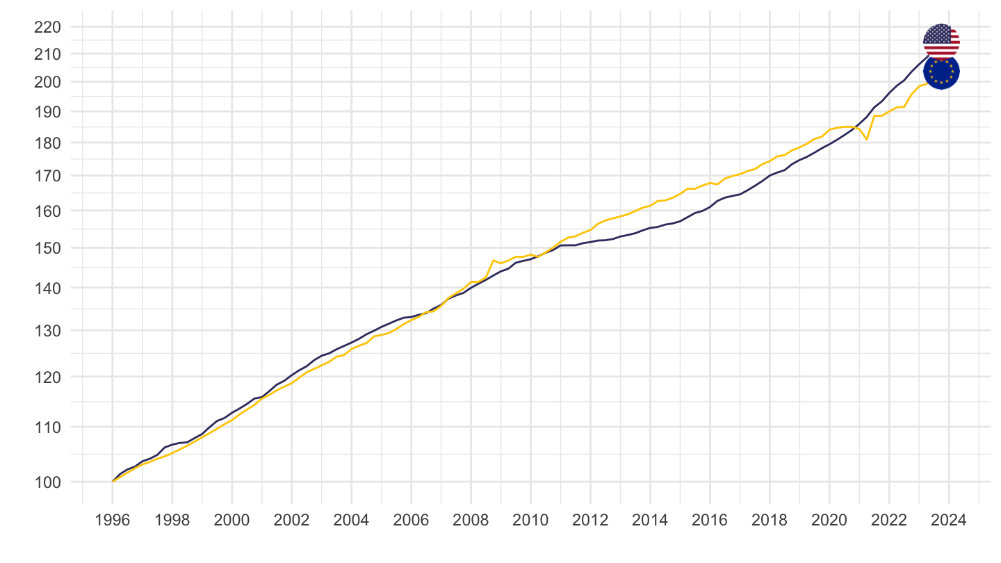
2019Q4
Quarterly
Code
HOU_EAR %>%
  filter(SECTOR == "S1",
         FREQ == "Q",
         REF_AREA %in% c("USA", "EA19", "FRA", "DEU"),
         ADJUSTMENT == "Y") %>%
  quarter_to_date %>%
  filter(date >= as.Date("2019-10-01")) %>%

  group_by(REF_AREA) %>%
  arrange(date) %>%
  mutate(obsValue = 100*obsValue/obsValue[1]) %>%
  mutate(Ref_area = ifelse(REF_AREA == "EA19", "Europe", Ref_area)) %>%
  left_join(colors, by = c("Ref_area" = "country")) %>%
  mutate(color = ifelse(REF_AREA == "EA19", color2, color)) %>%
  rename(Location = Ref_area) %>%
  ggplot(.) + geom_line(aes(x = date, y = obsValue, color = color)) +
  scale_color_identity() + theme_minimal() + add_4flags +
  scale_x_date(breaks = seq(1996, 2100, 1) %>% paste0("-01-01") %>% as.Date,
               labels = date_format("%Y")) +
  scale_y_log10(breaks = seq(10, 500, 2),
                     labels = scales::dollar_format(accuracy = 1, suffix = "", prefix = "")) +
  ylab("") + xlab("")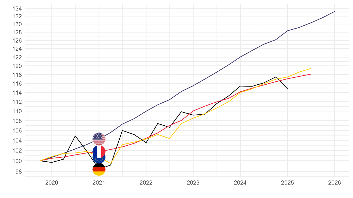
Quarterly
Code
HOU_EAR %>%
  filter(SECTOR == "S1",
         FREQ == "Q",
         REF_AREA %in% c("USA", "EA19", "FRA", "EU27_2020"),
         ADJUSTMENT == "Y") %>%
  quarter_to_date %>%
  filter(date >= as.Date("2019-10-01")) %>%

  group_by(REF_AREA) %>%
  arrange(date) %>%
  mutate(obsValue = 100*obsValue/obsValue[1]) %>%
  mutate(Ref_area = ifelse(REF_AREA == "EA19", "Europe", Ref_area)) %>%
  ggplot(.) + geom_line(aes(x = date, y = obsValue, color = Ref_area)) +
  theme_minimal() +
  scale_x_date(breaks = seq(1996, 2100, 1) %>% paste0("-01-01") %>% as.Date,
               labels = date_format("%Y")) +
  scale_y_log10(breaks = seq(10, 500, 2),
                     labels = scales::dollar_format(accuracy = 1, suffix = "", prefix = "")) +
  ylab("") + xlab("")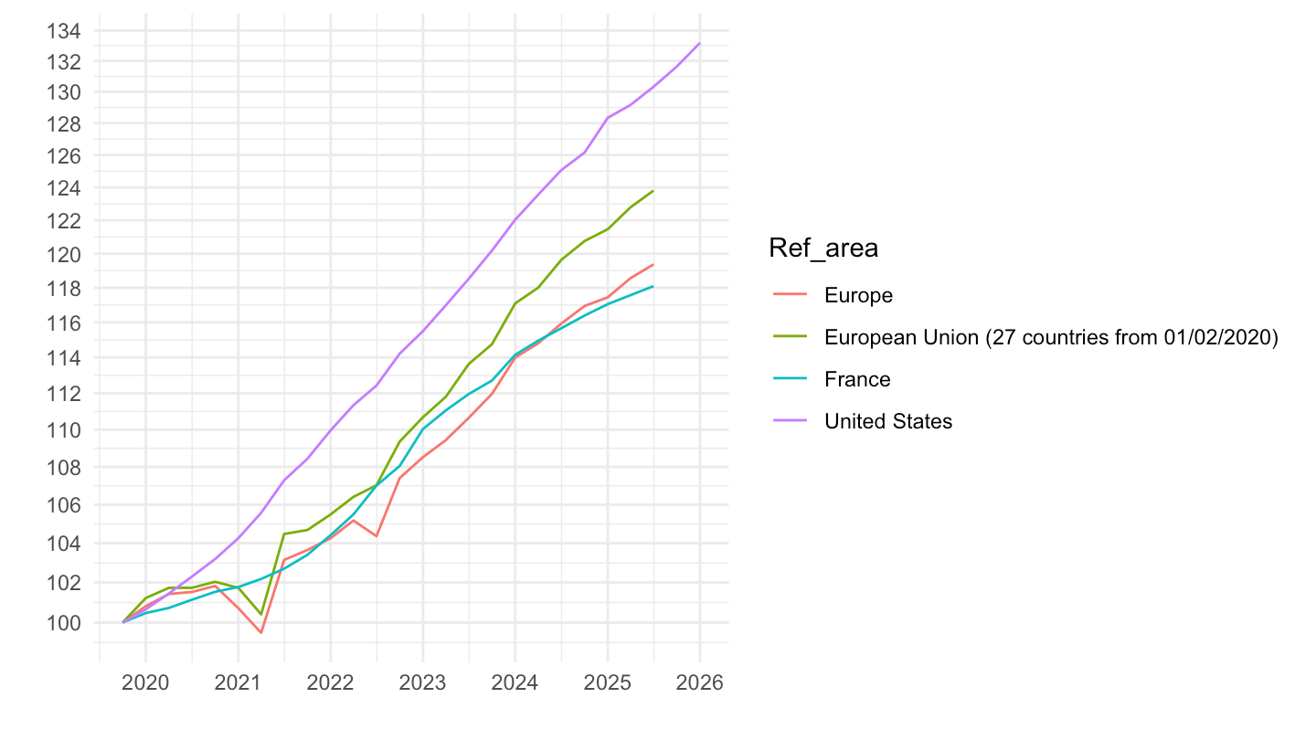
Monthly
Code
HOU_EAR %>%
  filter(SECTOR == "S1",
         FREQ == "M",
         REF_AREA %in% c("USA", "EA19"),
         ADJUSTMENT == "Y") %>%
  month_to_date %>%
  filter(date >= as.Date("1996-01-01")) %>%

  group_by(REF_AREA) %>%
  arrange(date) %>%
  mutate(obsValue = 100*obsValue/obsValue[1]) %>%
  mutate(Ref_area = ifelse(REF_AREA == "EA19", "Europe", Ref_area)) %>%
  left_join(colors, by = c("Ref_area" = "country")) %>%
  mutate(color = ifelse(REF_AREA == "EA19", color2, color)) %>%
  rename(Location = Ref_area) %>%
  ggplot(.) + geom_line(aes(x = date, y = obsValue, color = color)) +
  scale_color_identity() + theme_minimal() + add_2flags +
  scale_x_date(breaks = seq(1996, 2100, 2) %>% paste0("-01-01") %>% as.Date,
               labels = date_format("%Y")) +
  scale_y_log10(breaks = seq(10, 500, 10),
                     labels = scales::dollar_format(accuracy = 1, suffix = "", prefix = "")) +
  ylab("") + xlab("")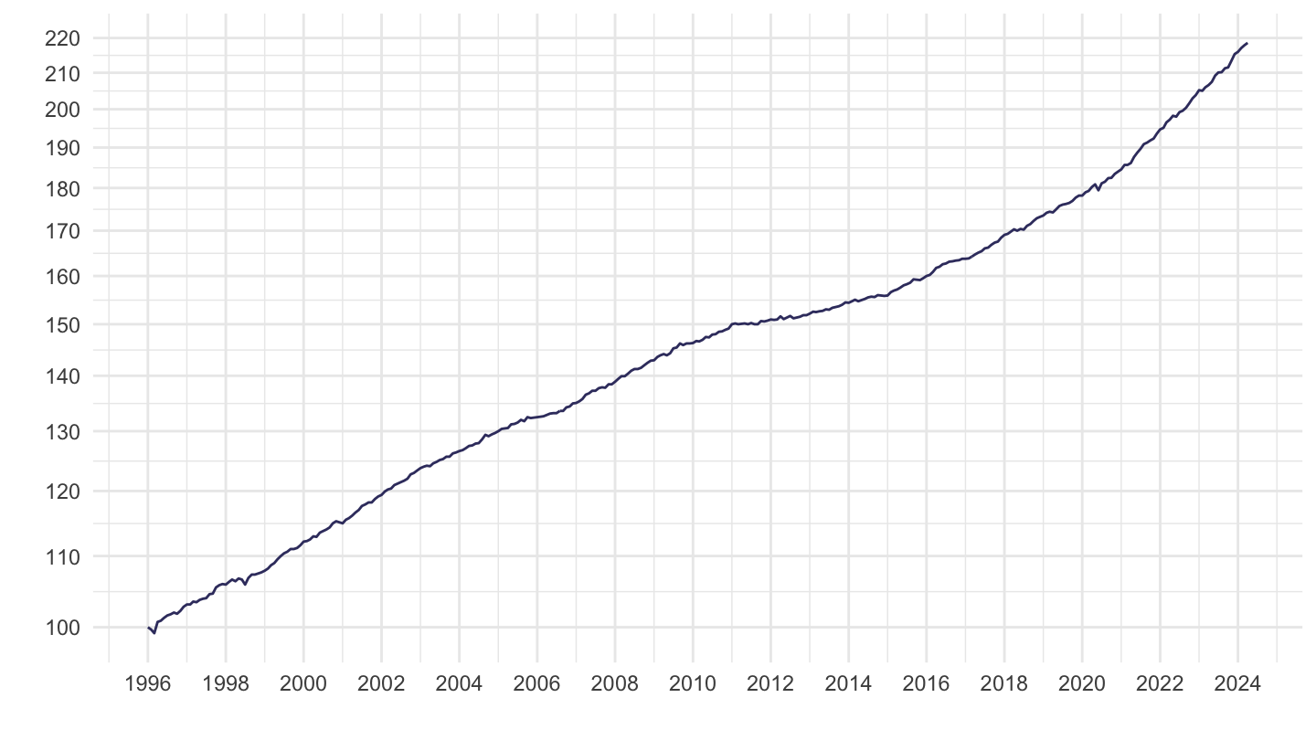
Eurozone, Japan, United States, United Kingdom
All
Code
HOU_EAR %>%
  filter(SECTOR == "S1",
         FREQ == "Q",
         REF_AREA %in% c("USA", "JPN", "EA19", "GBR", "HUN", "POL"),
         ADJUSTMENT == "Y") %>%
  quarter_to_date %>%

  mutate(Ref_area = ifelse(REF_AREA == "EA19", "Europe", Ref_area)) %>%
  left_join(colors, by = c("Ref_area" = "country")) %>%
  mutate(color = ifelse(REF_AREA == "EA19", color2, color)) %>%
  rename(Location = Ref_area) %>%
  ggplot(.) + geom_line(aes(x = date, y = obsValue, color = color)) +
  scale_color_identity() + theme_minimal() + add_6flags +
  scale_x_date(breaks = seq(1920, 2100, 2) %>% paste0("-01-01") %>% as.Date,
               labels = date_format("%Y")) +
  scale_y_log10(breaks = seq(10, 500, 10),
                     labels = scales::dollar_format(accuracy = 1, suffix = " k", prefix = "")) +
  ylab("") + xlab("")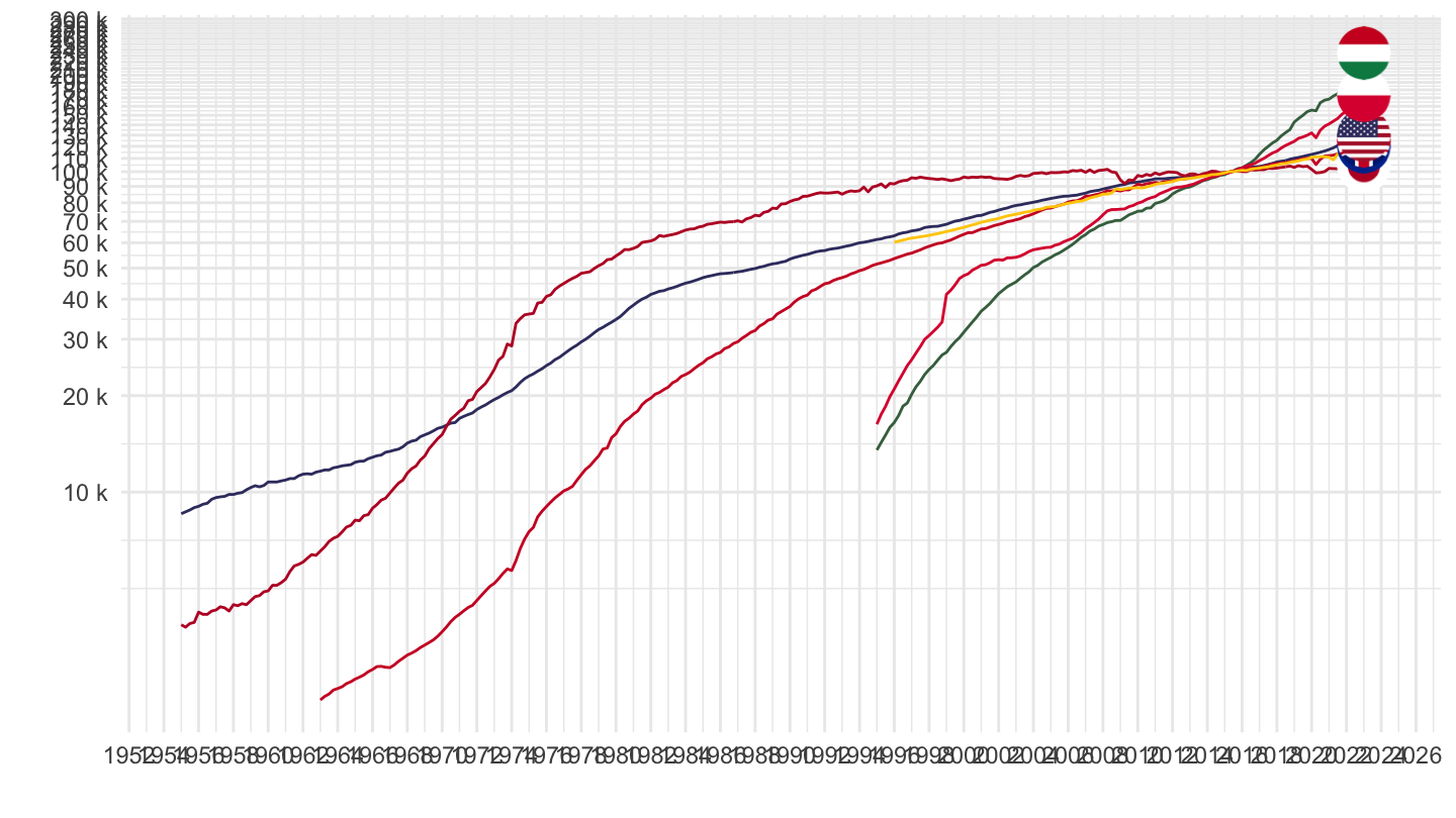
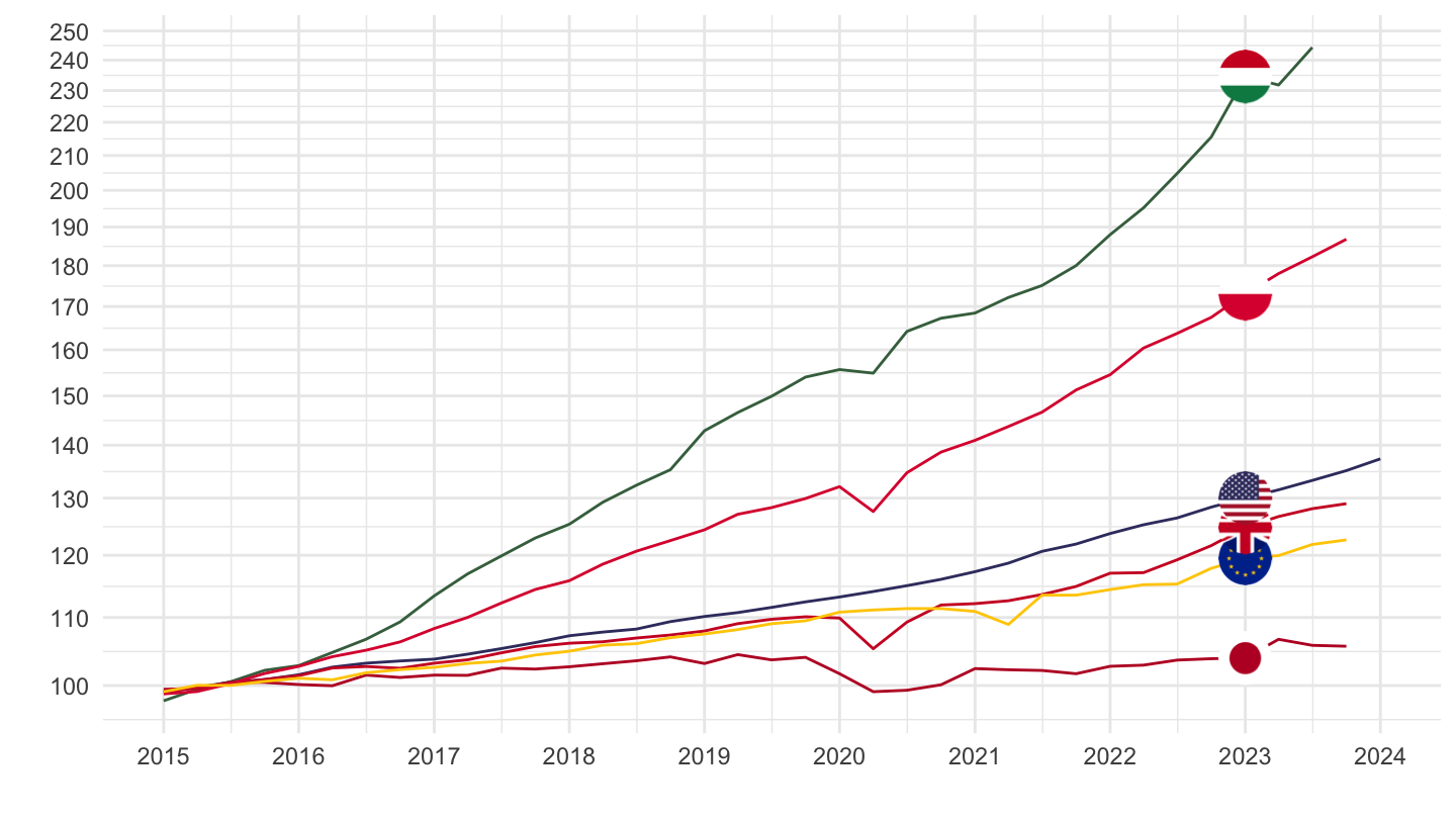
2015-
Code
HOU_EAR %>%
  filter(SECTOR == "S1",
         FREQ == "Q",
         REF_AREA %in% c("USA", "JPN", "EA19", "GBR", "HUN", "POL"),
         ADJUSTMENT == "Y") %>%
  quarter_to_date %>%
  filter(date >= as.Date("2015-01-01")) %>%

  mutate(Ref_area = ifelse(REF_AREA == "EA19", "Europe", Ref_area)) %>%
  left_join(colors, by = c("Ref_area" = "country")) %>%
  mutate(color = ifelse(REF_AREA == "EA19", color2, color)) %>%
  rename(Location = Ref_area) %>%
  ggplot(.) + geom_line(aes(x = date, y = obsValue, color = color)) +
  scale_color_identity() + theme_minimal() + add_6flags +
  scale_x_date(breaks = seq(1920, 2100, 1) %>% paste0("-01-01") %>% as.Date,
               labels = date_format("%Y")) +
  scale_y_log10(breaks = seq(10, 500, 10),
                     labels = scales::dollar_format(accuracy = 1, suffix = "", prefix = "")) +
  ylab("") + xlab("")