Comptes de secteurs institutionnels
Données - INSEE
Info
Last observation: 2026-Q1
First observation: 1949-Q1
Number of observations: 99 754
Last data update: 24 jul 2026, 01:17. Last compile: 24 jul 2026, 05:37
Structure
Données sur la macroéconomie en France
| source | dataset | Title | .html | .rData |
|---|---|---|---|---|
| bdf | CFT | Comptes Financiers Trimestriels | 2026-07-23 | 2025-03-09 |
| insee | CNA-2014-CONSO-SI | Dépenses de consommation finale par secteur institutionnel | 2026-07-23 | 2026-07-23 |
| insee | CNA-2014-CSI | Comptes des secteurs institutionnels | 2026-07-23 | 2026-07-23 |
| insee | CNA-2014-FBCF-BRANCHE | Formation brute de capital fixe (FBCF) par branche | 2026-07-23 | 2026-07-23 |
| insee | CNA-2014-FBCF-SI | Formation brute de capital fixe (FBCF) par secteur institutionnel | 2026-07-23 | 2026-07-23 |
| insee | CNA-2014-RDB | Revenu et pouvoir d’achat des ménages | 2026-07-23 | 2026-07-23 |
| insee | CNA-2020-CONSO-MEN | Consommation des ménages | 2026-07-23 | 2026-07-23 |
| insee | CNA-2020-PIB | Produit intérieur brut (PIB) et ses composantes | 2026-07-23 | 2026-07-23 |
| insee | CNT-2014-CB | Comptes des branches | 2026-07-23 | 2026-07-23 |
| insee | CNT-2014-CSI | Comptes de secteurs institutionnels | 2026-07-23 | 2026-07-22 |
| insee | CNT-2014-OPERATIONS | Opérations sur biens et services | 2026-07-23 | 2026-07-23 |
| insee | CNT-2014-PIB-EQB-RF | Équilibre du produit intérieur brut | 2026-07-23 | 2026-07-23 |
| insee | CONSO-MENAGES-2020 | Consommation des ménages en biens | 2026-07-23 | 2026-07-23 |
| insee | ICA-2015-IND-CONS | Indices de chiffre d'affaires dans l'industrie et la construction | 2026-07-23 | 2026-07-23 |
| insee | conso-mensuelle | Consommation de biens, données mensuelles | 2026-07-23 | 2023-07-04 |
| insee | t_1101 | 1.101 – Le produit intérieur brut et ses composantes à prix courants (En milliards d'euros) | 2026-07-23 | 2022-01-02 |
| insee | t_1102 | 1.102 – Le produit intérieur brut et ses composantes en volume aux prix de l'année précédente chaînés (En milliards d'euros 2014) | 2026-07-23 | 2020-10-30 |
| insee | t_1105 | 1.105 – Produit intérieur brut - les trois approches à prix courants (En milliards d'euros) - t_1105 | 2026-07-23 | 2020-10-30 |
Données
LAST_COMPILE
| LAST_COMPILE |
|---|
| 2026-07-24 |
Last
Code
`CNT-2020-CSI` %>%
  filter(TIME_PERIOD == max(TIME_PERIOD)) %>%
  select(TIME_PERIOD, TITLE_FR, OBS_VALUE) %>%
  arrange(TITLE_FR) %>%
  print_table_conditional()
Compte d’exploitation
Code
i_g("bib/insee/compte-d-exploitation.png")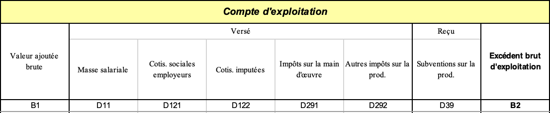
Ménages
Code
`CNT-2020-CSI` %>%
  filter(`SECT-INST` == "S14",
         TIME_PERIOD == "2021-Q4") %>%


  select_if(~ n_distinct(.) > 1) %>%
  select(OPERATION, Operation, INDICATEUR, Compte, OBS_VALUE) %>%
  print_table_conditional()
Revenu disponible brut des ménages
1949-
Code
`CNT-2020-CSI` %>%
  filter(`SECT-INST` == "S14",
         OPERATION %in% c("B6", "B7")) %>%

  quarter_to_date() %>%
  ggplot + geom_line(aes(x = date, y = OBS_VALUE, color = Operation)) +
  theme_minimal() +  xlab("") + ylab("") +
  scale_x_date(breaks = as.Date(paste0(seq(1940, 2100, 5), "-01-01")),
               labels = date_format("%Y")) +
  theme(legend.position = c(0.7, 0.2),
        legend.title = element_blank()) +
  scale_y_log10()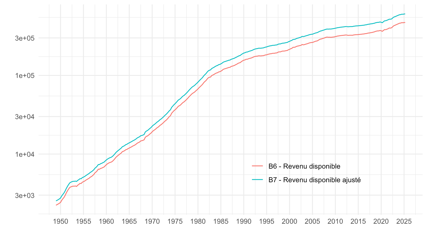
2017T2-
Code
`CNT-2020-CSI` %>%
  filter(`SECT-INST` == "S14",
         OPERATION %in% c("B6", "B7")) %>%

  quarter_to_date() %>%
  filter(date >= as.Date("2017-04-01")) %>%
  group_by(Operation) %>%
  arrange(date) %>%
  mutate(OBS_VALUE = 100*OBS_VALUE/OBS_VALUE[1]) %>%
  ggplot + geom_line(aes(x = date, y = OBS_VALUE, color = Operation)) +
  theme_minimal() +  xlab("") + ylab("") +
  scale_x_date(breaks = as.Date(paste0(seq(1940, 2100, 1), "-01-01")),
               labels = date_format("%Y")) +
  theme(legend.position = c(0.7, 0.2),
        legend.title = element_blank()) +
  scale_y_log10()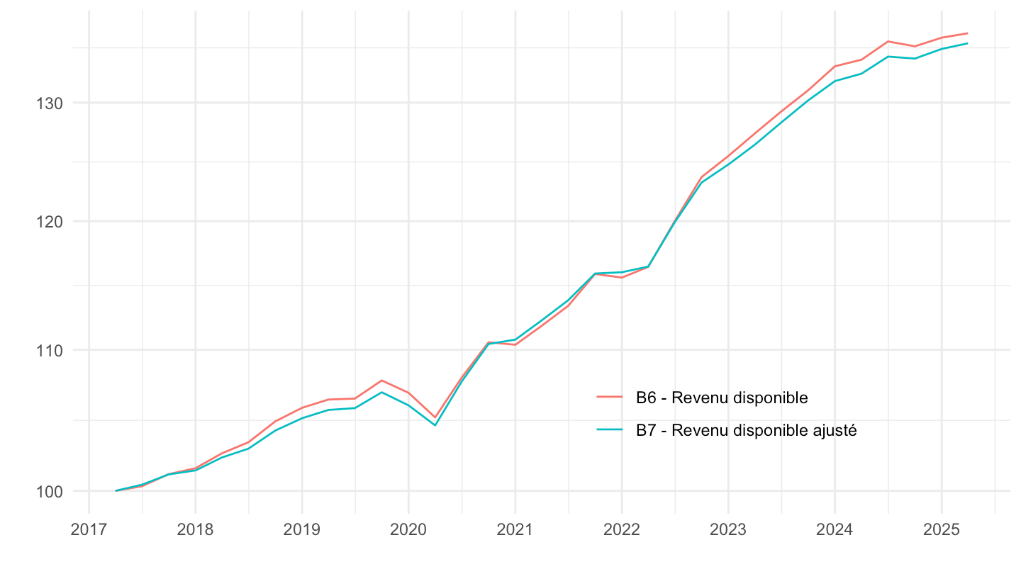
Secteurs
B9NF - Capacité (+) ou besoin (-) de financement
Code
`CNT-2020-CSI` %>%
  filter(OPERATION == "B9NF",
         FREQ == "T") %>%

  quarter_to_date %>%
  left_join(gdp_quarterly, by = "date") %>%
  ggplot + geom_line(aes(x = date, y = OBS_VALUE/gdp, color = `Sect-Inst`)) +
  theme_minimal() + xlab("") + ylab("% du PIB") +
  scale_x_date(breaks = seq(1940, 2100, 5) %>% paste0("-01-01") %>% as.Date,
               labels = date_format("%Y")) +
  scale_y_continuous(breaks = 0.01*seq(-100, 500, 2),
                labels = percent_format(accuracy = 1)) +
  theme(legend.position = c(0.6, 0.8),
        legend.title = element_blank()) +
  geom_hline(yintercept = 0, linetype = "dashed")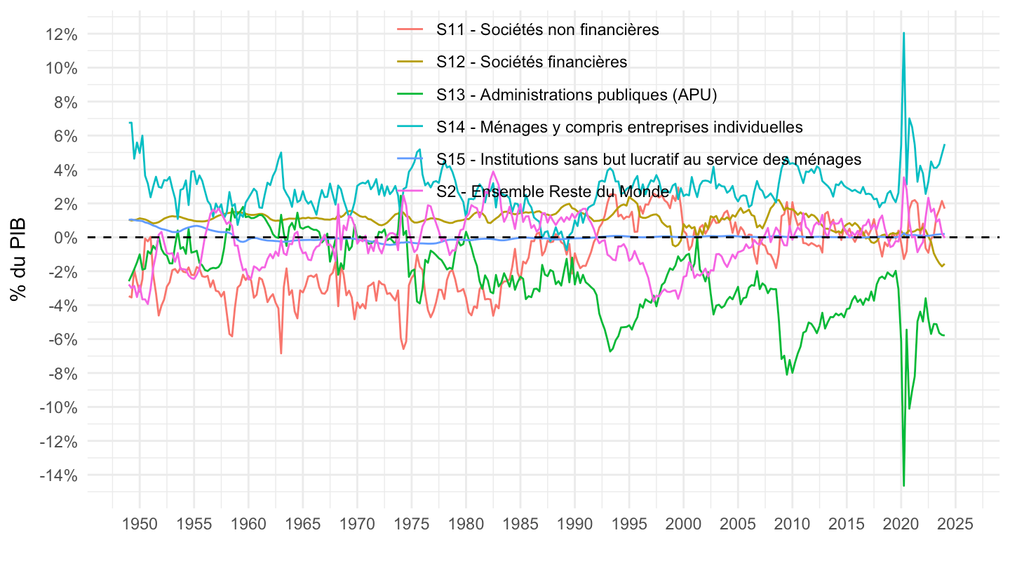
B2 - Excédent brut d’exploitation
Tous
Code
`CNT-2020-CSI` %>%
  filter(OPERATION == "B2",
         FREQ == "T") %>%

  quarter_to_date %>%
  left_join(gdp_quarterly, by = "date") %>%
  ggplot + geom_line(aes(x = date, y = OBS_VALUE/gdp, color = `Sect-Inst`)) +
  theme_minimal() + xlab("") + ylab("% du PIB") +
  scale_x_date(breaks = seq(1940, 2100, 5) %>% paste0("-01-01") %>% as.Date,
               labels = date_format("%Y")) +
  scale_y_continuous(breaks = 0.01*seq(-100, 500, 2),
                labels = percent_format(accuracy = 1)) +
  theme(legend.position = c(0.6, 0.7),
        legend.title = element_blank()) +
  geom_hline(yintercept = 0, linetype = "dashed")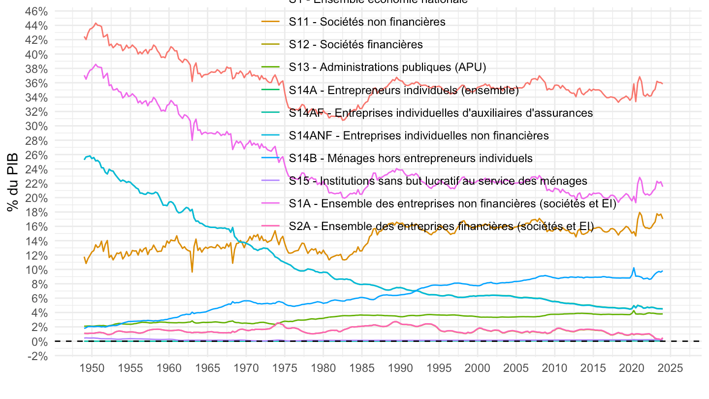
S1A, S1, S2A
Code
`CNT-2020-CSI` %>%
  filter(OPERATION == "B2",
        `SECT-INST` %in% c("S1A", "S1", "S2A"),
         FREQ == "T") %>%

  quarter_to_date %>%
  left_join(gdp_quarterly, by = "date") %>%
  ggplot + geom_line(aes(x = date, y = OBS_VALUE/gdp, color = `Sect-Inst`)) +
  theme_minimal() + xlab("") + ylab("% du PIB") +
  scale_x_date(breaks = seq(1940, 2100, 5) %>% paste0("-01-01") %>% as.Date,
               labels = date_format("%Y")) +
  scale_y_continuous(breaks = 0.01*seq(-100, 500, 2),
                labels = percent_format(accuracy = 1)) +
  theme(legend.position = c(0.6, 0.9),
        legend.title = element_blank()) +
  geom_hline(yintercept = 0, linetype = "dashed")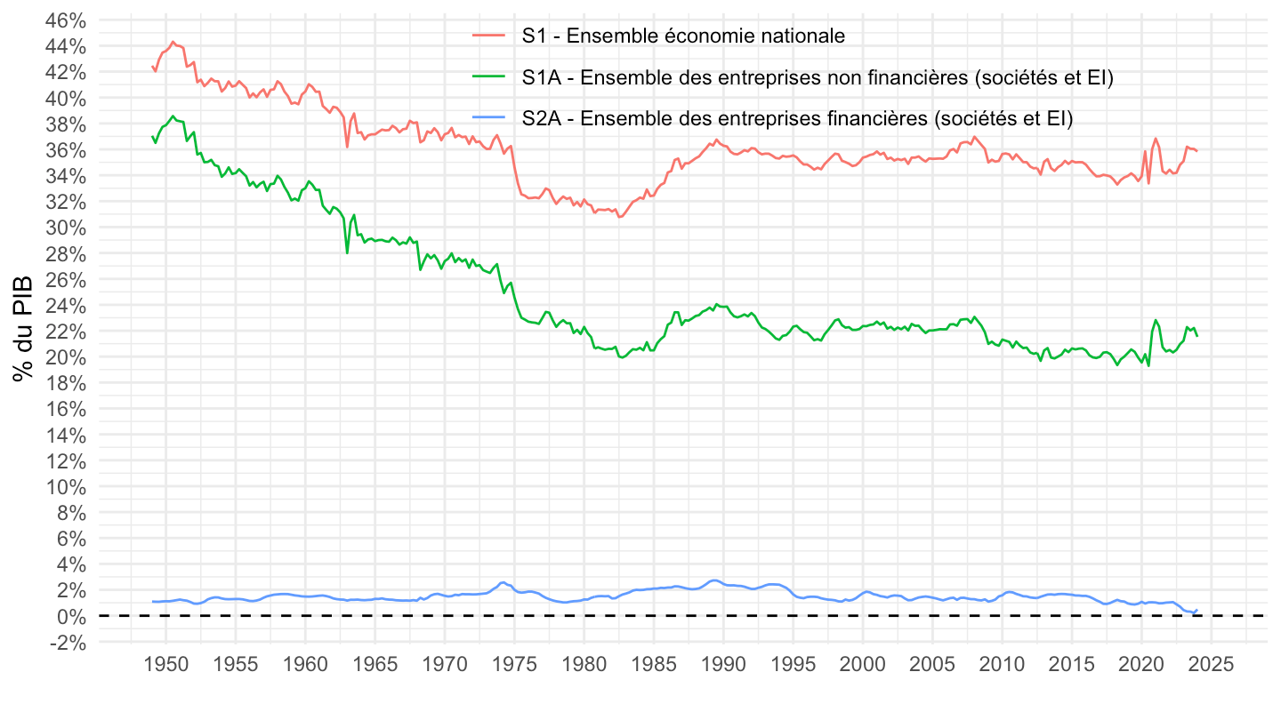
% de la VA du secteur
All
Code
`CNT-2020-CSI` %>%
  filter(OPERATION %in% c("B2", "B1")) %>%


  quarter_to_date() %>%
  select(date, OBS_VALUE, OPERATION, `SECT-INST`, `Sect-Inst`) %>%
  spread(OPERATION, OBS_VALUE) %>%
  ggplot + geom_line(aes(x = date, y = B2/B1, color = `Sect-Inst`)) +
  theme_minimal() +  xlab("") + ylab("Excédent d'exploitation / VA") +
  scale_x_date(breaks = as.Date(paste0(seq(1940, 2100, 5), "-01-01")),
               labels = date_format("%Y")) +
  scale_y_continuous(breaks = 0.01*seq(0, 100, 5),
                     labels = scales::percent_format(accuracy = 1)) +
  theme(legend.position = c(0.6, 0.7),
        legend.title = element_blank())
S1A, S1, S2A
Code
`CNT-2020-CSI` %>%
  filter(OPERATION %in% c("B2", "B1"),
        `SECT-INST` %in% c("S1A", "S1", "S2A")) %>%


  quarter_to_date() %>%
  select(date, OBS_VALUE, OPERATION, `SECT-INST`, `Sect-Inst`) %>%
  spread(OPERATION, OBS_VALUE) %>%
  ggplot + geom_line(aes(x = date, y = B2/B1, color = `Sect-Inst`)) +
  theme_minimal() +  xlab("") + ylab("Excédent d'exploitation / VA") +
  scale_x_date(breaks = as.Date(paste0(seq(1940, 2100, 5), "-01-01")),
               labels = date_format("%Y")) +
  scale_y_continuous(breaks = 0.01*seq(0, 100, 5),
                     labels = scales::percent_format(accuracy = 1)) +
  theme(legend.position = c(0.35, 0.2),
        legend.title = element_blank())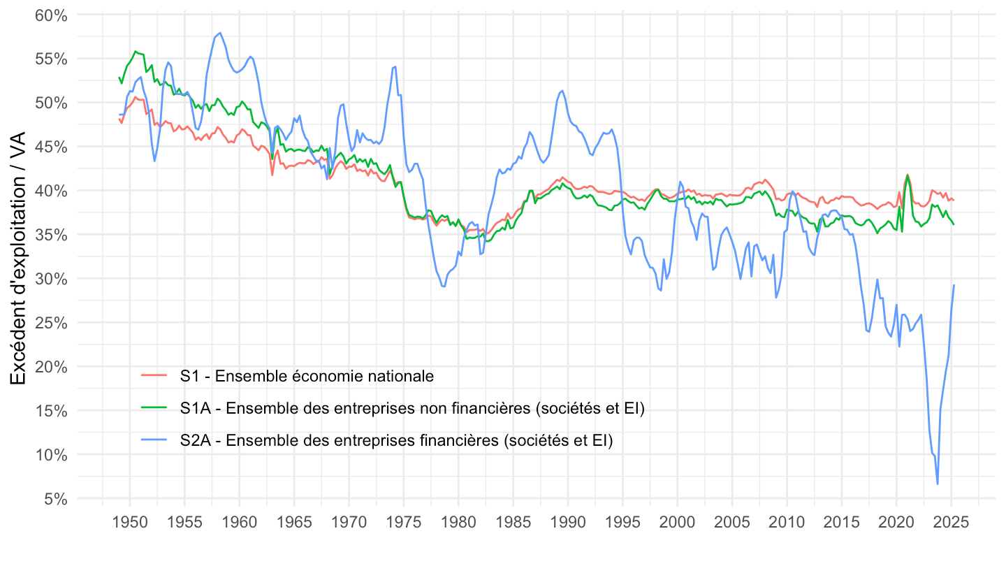
S11, S12, S14
Code
`CNT-2020-CSI` %>%
  filter(OPERATION == "B9NF",
         FREQ == "T",
         `SECT-INST` %in% c("S11", "S12", "S14")) %>%

  quarter_to_date %>%
  left_join(gdp_quarterly, by = "date") %>%
  ggplot + geom_line(aes(x = date, y = OBS_VALUE/gdp, color = `Sect-Inst`)) +
  theme_minimal() + xlab("") + ylab("% du PIB") +
  scale_x_date(breaks = seq(1940, 2100, 5) %>% paste0("-01-01") %>% as.Date,
               labels = date_format("%Y")) +
  scale_y_continuous(breaks = 0.01*seq(-100, 500, 2),
                labels = percent_format(accuracy = 1)) +
  theme(legend.position = c(0.6, 0.9),
        legend.title = element_blank()) +
  geom_hline(yintercept = 0, linetype = "dashed")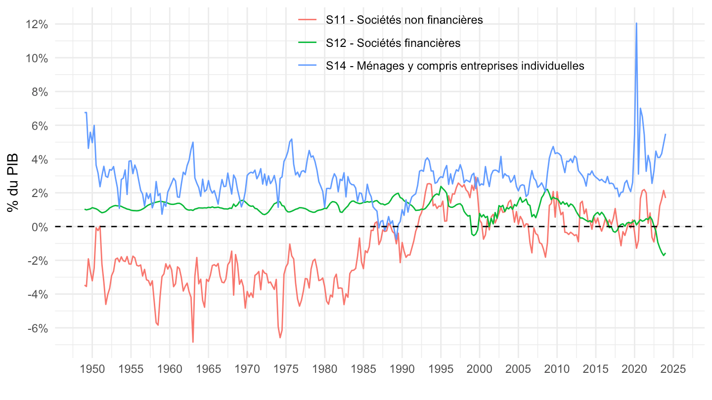
S12 - Sociétés financières
D1/B1G - Rémunération des salariés
Code
`CNT-2020-CSI` %>%
  filter(`SECT-INST` == "S12",
         OPERATION %in% c("D1", "B1")) %>%
  quarter_to_date() %>%
  select(date, OBS_VALUE, OPERATION) %>%
  spread(OPERATION, OBS_VALUE) %>%
  ggplot + geom_line(aes(x = date, y = D1/B1)) +
  theme_minimal() +  xlab("") + ylab("Part de la rémunération des salariés des SNF") +
  scale_x_date(breaks = as.Date(paste0(seq(1940, 2100, 5), "-01-01")),
               labels = date_format("%Y")) +
  scale_y_continuous(breaks = 0.01*seq(-0, 90, 5),
                     labels = scales::percent_format(accuracy = 1))
B2/B1G - Excédent d’exploitation
Code
`CNT-2020-CSI` %>%
  filter(`SECT-INST` == "S12",
         OPERATION %in% c("B2", "B1")) %>%
  quarter_to_date() %>%
  select(date, OBS_VALUE, OPERATION) %>%
  spread(OPERATION, OBS_VALUE) %>%
  ggplot + geom_line(aes(x = date, y = B2/B1)) +
  theme_minimal() +  xlab("") + ylab("") +
  scale_x_date(breaks = as.Date(paste0(seq(1940, 2100, 5), "-01-01")),
               labels = date_format("%Y")) +
  scale_y_continuous(breaks = 0.01*seq(0, 90, 5),
                     labels = scales::percent_format(accuracy = 1))
(D292+D39)/B1
All
Code
`CNT-2020-CSI` %>%
  filter(`SECT-INST` == "S12",
         OPERATION %in% c("D292", "B1", "D39")) %>%
  quarter_to_date() %>%
  select(date, OBS_VALUE, OPERATION) %>%
  spread(OPERATION, OBS_VALUE) %>%
  ggplot + geom_line(aes(x = date, y = (D292+D39)/B1)) +
  theme_minimal() +  xlab("") + ylab("Impôts - Subventions sur la production") +
  scale_x_date(breaks = as.Date(paste0(seq(1940, 2100, 5), "-01-01")),
               labels = date_format("%Y")) +
  scale_y_continuous(breaks = 0.01*seq(-2, 90, 1),
                     labels = scales::percent_format(accuracy = 1)) +
  geom_hline(yintercept = 0, linetype = "dashed", color = "red")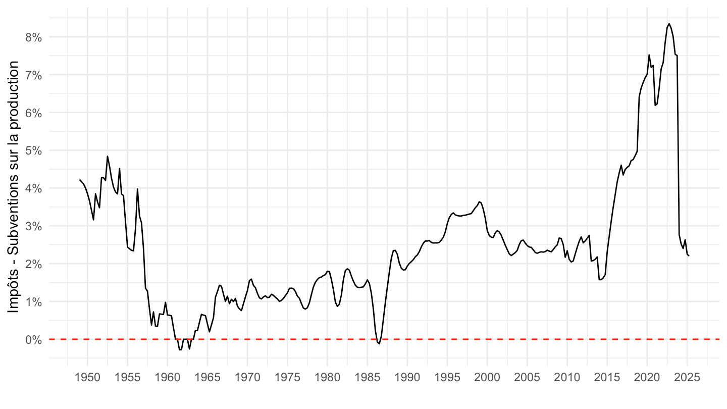
2000-
Code
`CNT-2020-CSI` %>%
  filter(`SECT-INST` == "S12",
         OPERATION %in% c("D292", "B1", "D39")) %>%
  quarter_to_date() %>%
  filter(date >= as.Date("2000-01-01")) %>%
  select(date, OBS_VALUE, OPERATION) %>%
  spread(OPERATION, OBS_VALUE) %>%
  ggplot + geom_line(aes(x = date, y = (D292+D39)/B1)) +
  theme_minimal() +  xlab("") + ylab("Impôts - Subventions sur la production") +
  scale_x_date(breaks = as.Date(paste0(seq(1940, 2100, 5), "-01-01")),
               labels = date_format("%Y")) +
  scale_y_continuous(breaks = 0.01*seq(-2, 90, 1),
                     labels = scales::percent_format(accuracy = 1)) +
  geom_hline(yintercept = 0, linetype = "dashed", color = "red")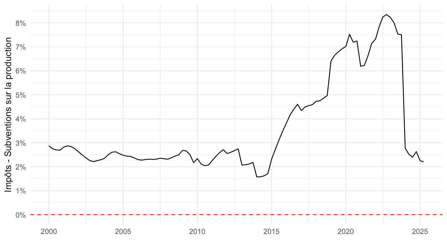
Investissement et taux de marge
Investissement total
Code
`CNT-2020-PIB-EQB-RF` %>%
  filter(FREQ == "T",
         VALORISATION == "V",
         OPERATION %in% c( "P51", "PIB")) %>%
  quarter_to_date %>%
  select(date, OPERATION, OBS_VALUE) %>%
  spread(OPERATION, OBS_VALUE) %>%
  transmute(date,
         value = P51/PIB,
         Variable = "Investissement (% du PIB)") %>%
  bind_rows(`CNT-2020-CSI` %>%
              filter(`SECT-INST` == "S11",
                     OPERATION %in% c("B2", "B1")) %>%
              quarter_to_date() %>%
              select(date, OBS_VALUE, OPERATION) %>%
              spread(OPERATION, OBS_VALUE) %>%
              transmute(date, value = B2/B1,
                        Variable = "Taux de marge")) %>%
  ggplot(.) + theme_minimal() + ylab("") + xlab("") +
  geom_line(aes(x = date, y = value, color = Variable)) +
  theme(legend.title = element_blank(),
        legend.position = c(0.3, 0.9)) +
  scale_x_date(breaks = seq(1950, 2100, 10) %>% paste0("-01-01") %>% as.Date,
               labels = date_format("%Y")) +
  scale_color_manual(values = viridis(3)[1:2]) +
  scale_y_continuous(breaks = 0.01*seq(0, 100, 2),
                     labels = scales::percent_format(accuracy = 1)) +
    geom_rect(data = data_frame(start = as.Date("1983-01-01"),
                                end = as.Date("1992-12-31")),
              aes(xmin = start, xmax = end, ymin = -Inf, ymax = +Inf),
              fill = viridis(4)[4], alpha = 0.2)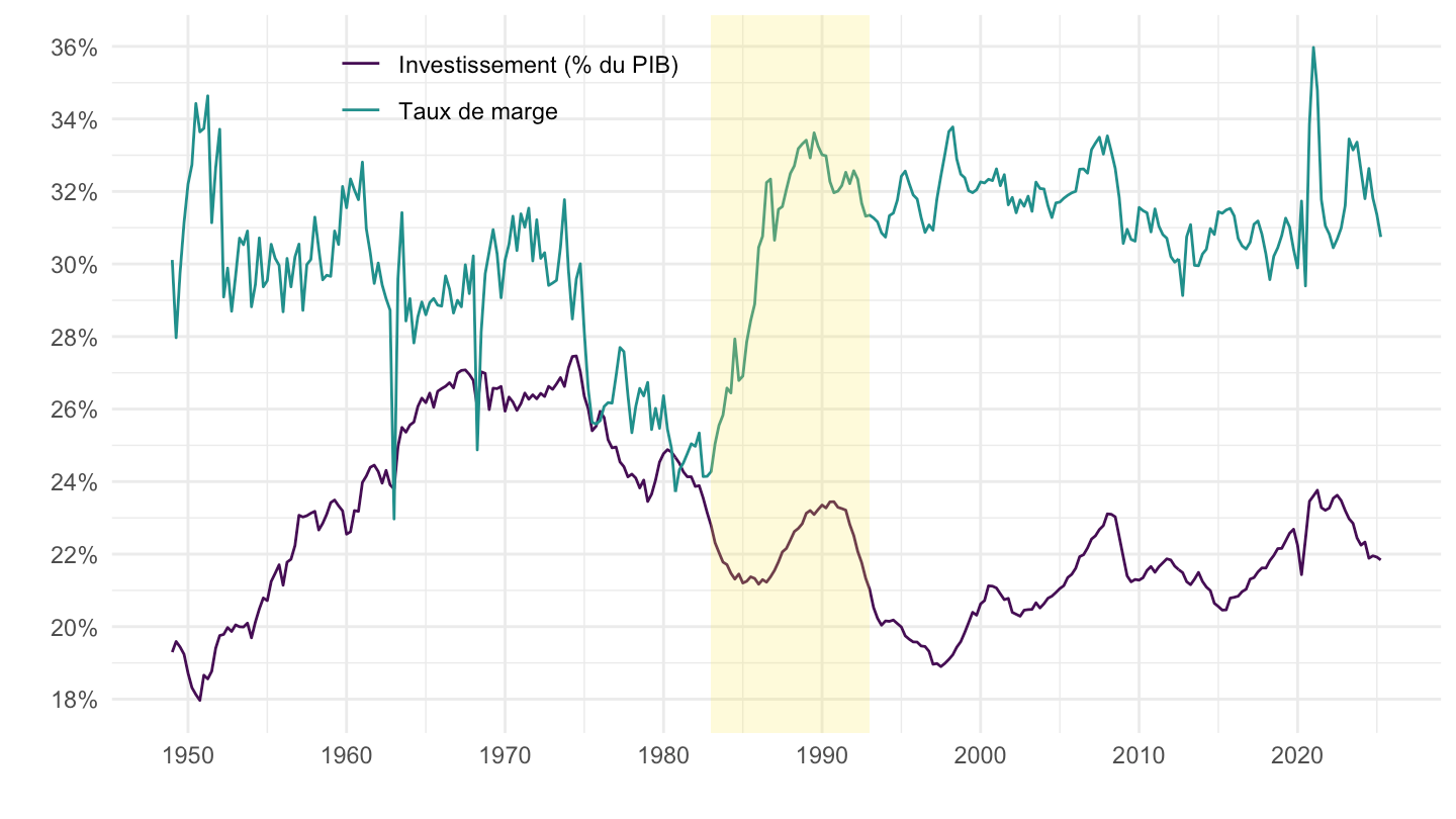
Sociétés non Financières
Tous
Code
`CNT-2020-PIB-EQB-RF` %>%
  filter(FREQ == "T",
         VALORISATION == "V",
         OPERATION %in% c( "P51S", "PIB")) %>%
  quarter_to_date %>%
  select(date, OPERATION, OBS_VALUE) %>%
  spread(OPERATION, OBS_VALUE) %>%
  transmute(date,
         value = P51S/PIB,
         Variable = "Investissement des Sociétés non Financières (% du PIB)") %>%
  bind_rows(`CNT-2020-CSI` %>%
              filter(`SECT-INST` == "S11",
                     OPERATION %in% c("B2", "B1")) %>%
              quarter_to_date() %>%
              select(date, OBS_VALUE, OPERATION) %>%
              spread(OPERATION, OBS_VALUE) %>%
              transmute(date, value = B2/B1,
                        Variable = "Taux de marge des Sociétés non Financières")) %>%
  ggplot(.) + theme_minimal() + ylab("") + xlab("") +
  geom_line(aes(x = date, y = value, color = Variable)) +
  theme(legend.title = element_blank(),
        legend.position = c(0.3, 0.35)) +
  scale_x_date(breaks = seq(1950, 2100, 10) %>% paste0("-01-01") %>% as.Date,
               labels = date_format("%Y")) +
  scale_color_manual(values = viridis(3)[1:2]) +
  scale_y_continuous(breaks = 0.01*seq(0, 100, 2),
                     labels = scales::percent_format(accuracy = 1)) +
    geom_rect(data = data_frame(start = as.Date("1983-01-01"),
                                end = as.Date("1992-12-31")),
              aes(xmin = start, xmax = end, ymin = -Inf, ymax = +Inf),
              fill = viridis(4)[4], alpha = 0.2)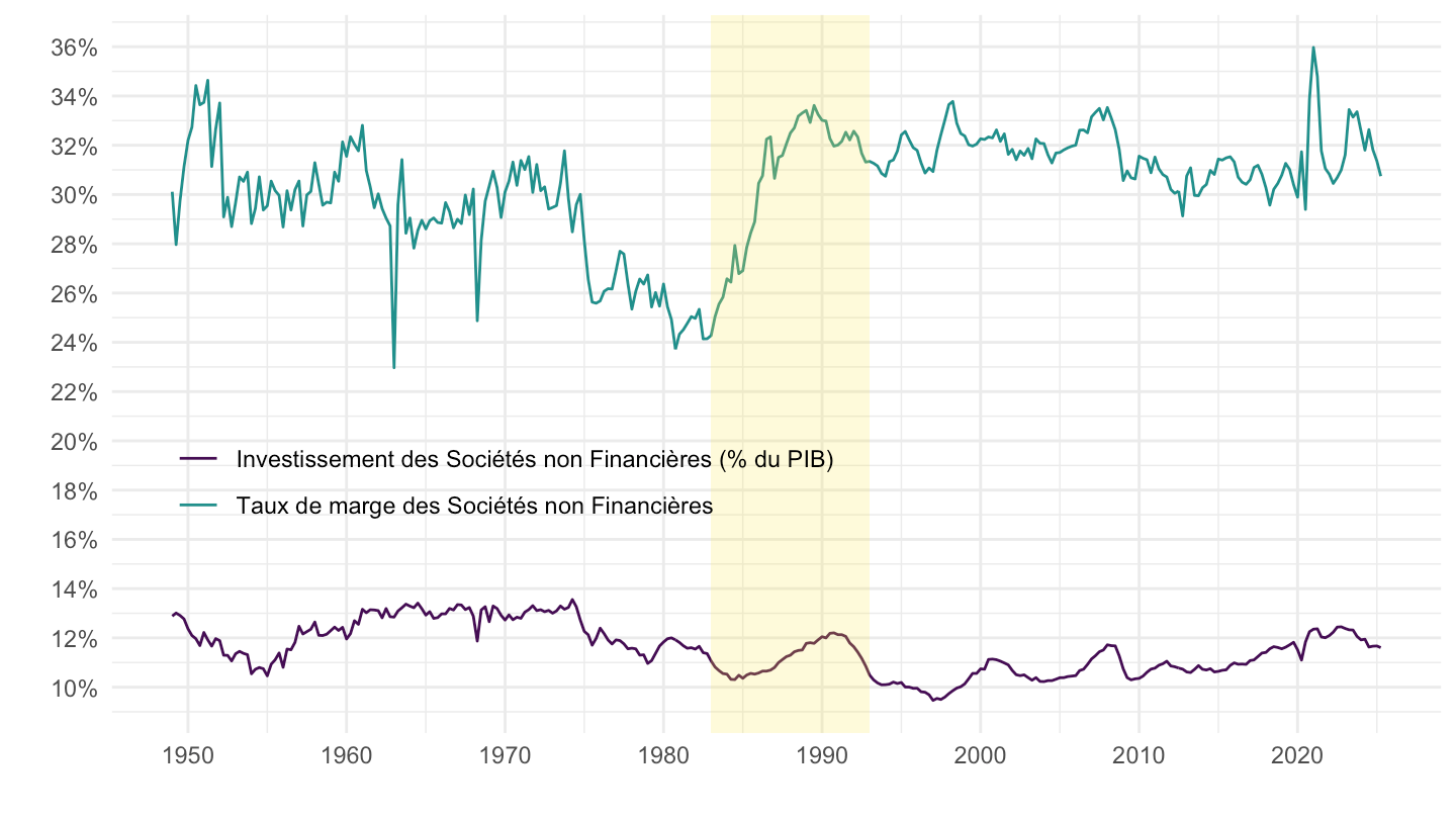
Marges: comparer différents secteurs
B2/B1G - Excédent d’exploitation
S1A - Entreprises non financières
B2/B1G - Excédent d’exploitation
All
Code
`CNT-2020-CSI` %>%
  filter(`SECT-INST` == "S1A",
         OPERATION %in% c("B2", "B1")) %>%

  quarter_to_date() %>%
  select(date, OBS_VALUE, OPERATION) %>%
  spread(OPERATION, OBS_VALUE) %>%
  ggplot + geom_line(aes(x = date, y = B2/B1)) +
  theme_minimal() +  xlab("") + ylab("Excédent d'exploitation / VA, Sociétés non financières") +
  scale_x_date(breaks = as.Date(paste0(seq(1940, 2100, 5), "-01-01")),
               labels = date_format("%Y")) +
  scale_y_continuous(breaks = 0.01*seq(-2, 90, 1),
                     labels = scales::percent_format(accuracy = 1)) +
    geom_rect(data = data_frame(start = as.Date("2017-07-01"),
                                end = as.Date("2021-12-31")),
              aes(xmin = start, xmax = end, ymin = -Inf, ymax = +Inf),
              fill = viridis(4)[4], alpha = 0.2)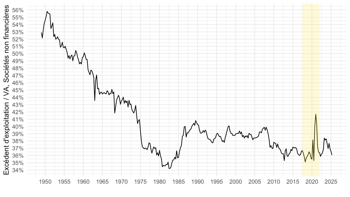
5 ans
Code
`CNT-2020-CSI` %>%
  filter(`SECT-INST` == "S1A",
         OPERATION %in% c("B2", "B1")) %>%

  quarter_to_date() %>%
  select(date, OBS_VALUE, OPERATION) %>%
  spread(OPERATION, OBS_VALUE) %>%
  mutate(obsValue = B2/B1,
         obsValue_mean = zoo::rollmean(obsValue, 16, fill = NA, align = "right")) %>%
  ggplot + geom_line(aes(x = date, y = obsValue_mean)) +
  theme_minimal() +  xlab("") + ylab("Excédent d'exploitation / VA, SNF, moyenne sur 4 ans") +
  scale_x_date(breaks = as.Date(paste0(seq(1940, 2100, 5), "-01-01")),
               labels = date_format("%Y")) +
  scale_y_continuous(breaks = 0.01*seq(-2, 90, 1),
                     labels = scales::percent_format(accuracy = 1)) +
    geom_rect(data = data_frame(start = as.Date("2014-08-26"),
                                end = as.Date("2021-12-31")),
              aes(xmin = start, xmax = end, ymin = -Inf, ymax = +Inf),
              fill = viridis(4)[4], alpha = 0.2) +
  geom_vline(xintercept = as.Date("2014-08-26"), linetype = "dashed") +
  geom_vline(xintercept = as.Date("2017-05-07"), linetype = "dashed")
S11 - Sociétés non financières
D1/B1G - Rémunération des salariés
Code
`CNT-2020-CSI` %>%
  filter(`SECT-INST` == "S11",
         OPERATION %in% c("D1", "B1")) %>%
  quarter_to_date() %>%
  select(date, OBS_VALUE, OPERATION) %>%
  spread(OPERATION, OBS_VALUE) %>%
  ggplot + geom_line(aes(x = date, y = D1/B1)) +
  theme_minimal() +  xlab("") + ylab("Part de la rémunération des salariés des SNF") +
  scale_x_date(breaks = as.Date(paste0(seq(1940, 2100, 5), "-01-01")),
               labels = date_format("%Y")) +
  scale_y_continuous(breaks = 0.01*seq(-2, 90, 1),
                     labels = scales::percent_format(accuracy = 1))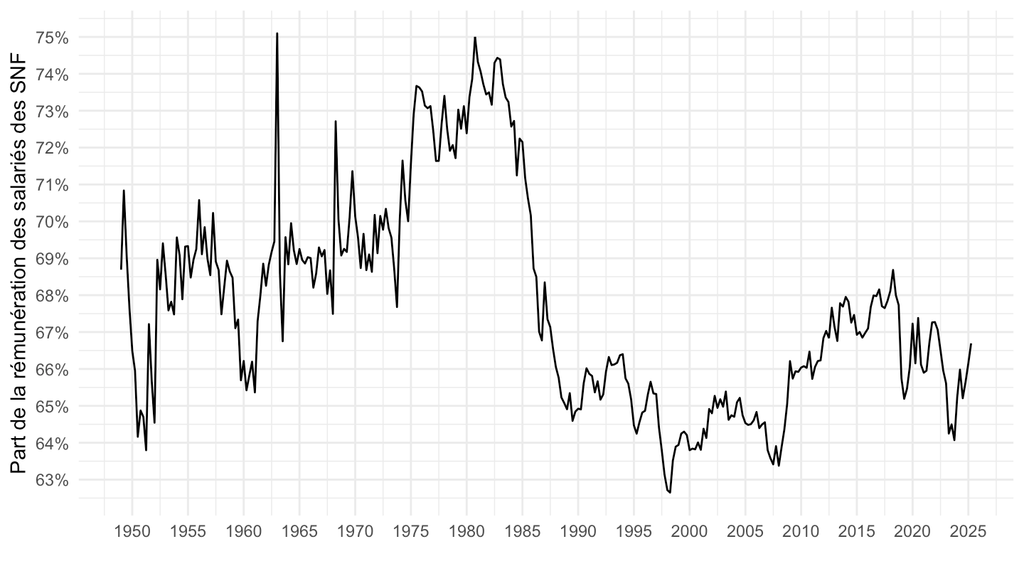
B2/B1G - Excédent d’exploitation
Taux de marge en 2021
Code
ig_b("insee", "ENTFRA23", "F9", "table1")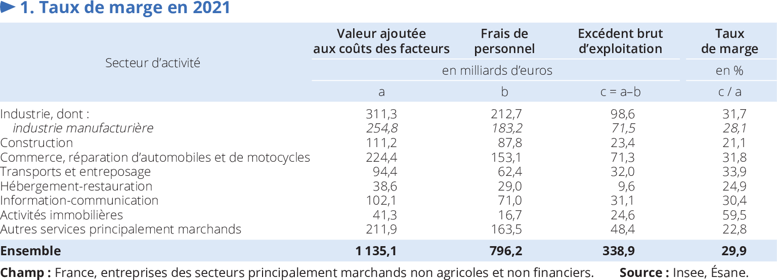
All
1949-
Code
`CNT-2020-CSI` %>%
  filter(`SECT-INST` == "S11",
         OPERATION %in% c("B2", "B1")) %>%

  quarter_to_date() %>%
  select(date, OBS_VALUE, OPERATION) %>%
  spread(OPERATION, OBS_VALUE) %>%
  mutate(value = B2/B1) %>%
  ggplot + geom_line(aes(x = date, y = value)) +
  theme_minimal() +  xlab("") + ylab("Excédent d'exploitation / VA, Sociétés non financières") +
  scale_x_date(breaks = as.Date(paste0(seq(1940, 2100, 5), "-01-01")),
               labels = date_format("%Y")) +
  scale_y_continuous(breaks = 0.01*seq(-2, 90, 1),
                     labels = scales::percent_format(accuracy = 1))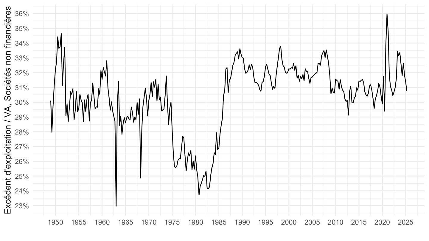
1990-
Code
`CNT-2020-CSI` %>%
  filter(`SECT-INST` == "S11",
         OPERATION %in% c("B2", "B1")) %>%

  quarter_to_date() %>%
  filter(date >= as.Date("1990-01-01")) %>%
  select(date, OBS_VALUE, OPERATION) %>%
  spread(OPERATION, OBS_VALUE) %>%
  mutate(value = B2/B1) %>%
  ggplot + geom_line(aes(x = date, y = value)) +
  theme_minimal() +  xlab("") + ylab("Excédent d'exploitation / VA, Sociétés non financières") +
  scale_x_date(breaks = as.Date(paste0(seq(1940, 2100, 5), "-01-01")),
               labels = date_format("%Y")) +
  scale_y_continuous(breaks = 0.01*seq(-2, 90, 1),
                     labels = scales::percent_format(accuracy = 1))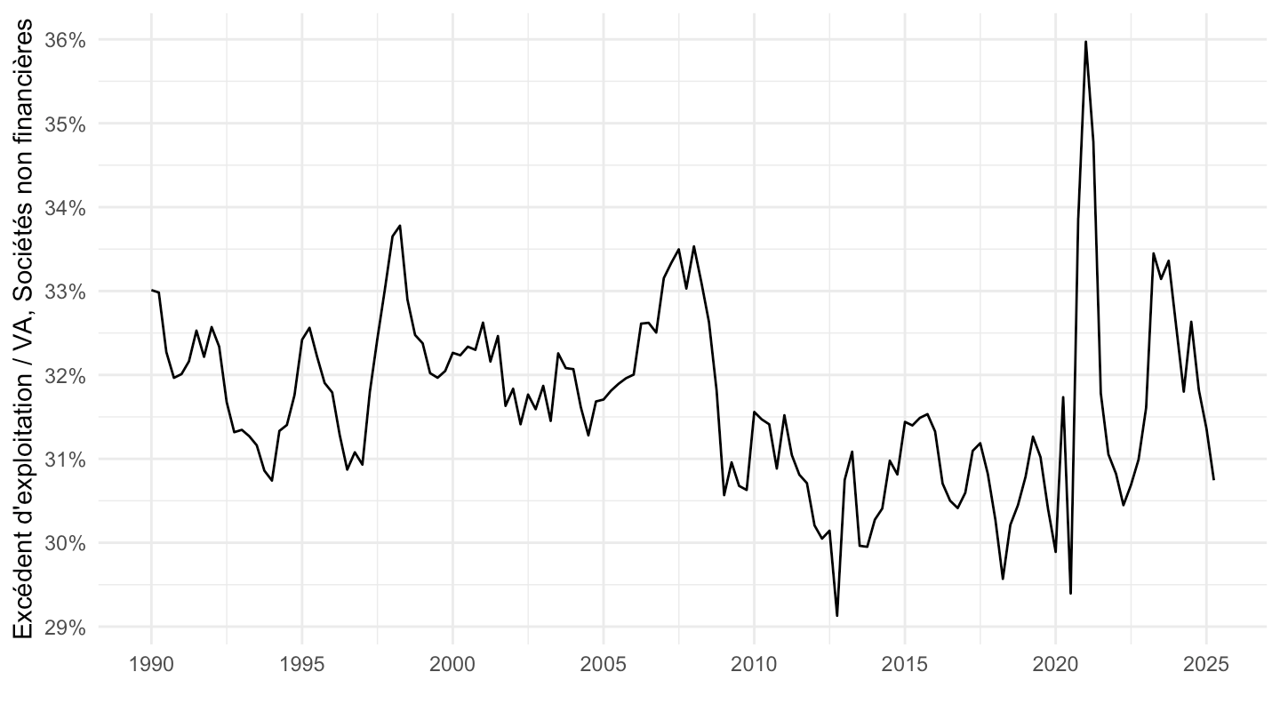
2010-
Code
`CNT-2020-CSI` %>%
  filter(`SECT-INST` == "S11",
         OPERATION %in% c("B2", "B1")) %>%

  quarter_to_date() %>%
  filter(date >= as.Date("2010-01-01")) %>%
  select(date, OBS_VALUE, OPERATION) %>%
  spread(OPERATION, OBS_VALUE) %>%
  mutate(value = B2/B1) %>%
  ggplot + geom_line(aes(x = date, y = value)) +
  theme_minimal() +  xlab("") + ylab("Excédent d'exploitation / VA, Sociétés non financières") +
  scale_x_date(breaks = as.Date(paste0(seq(1940, 2100, 5), "-01-01")),
               labels = date_format("%Y")) +
  scale_y_continuous(breaks = 0.01*seq(-2, 90, 1),
                     labels = scales::percent_format(accuracy = 1))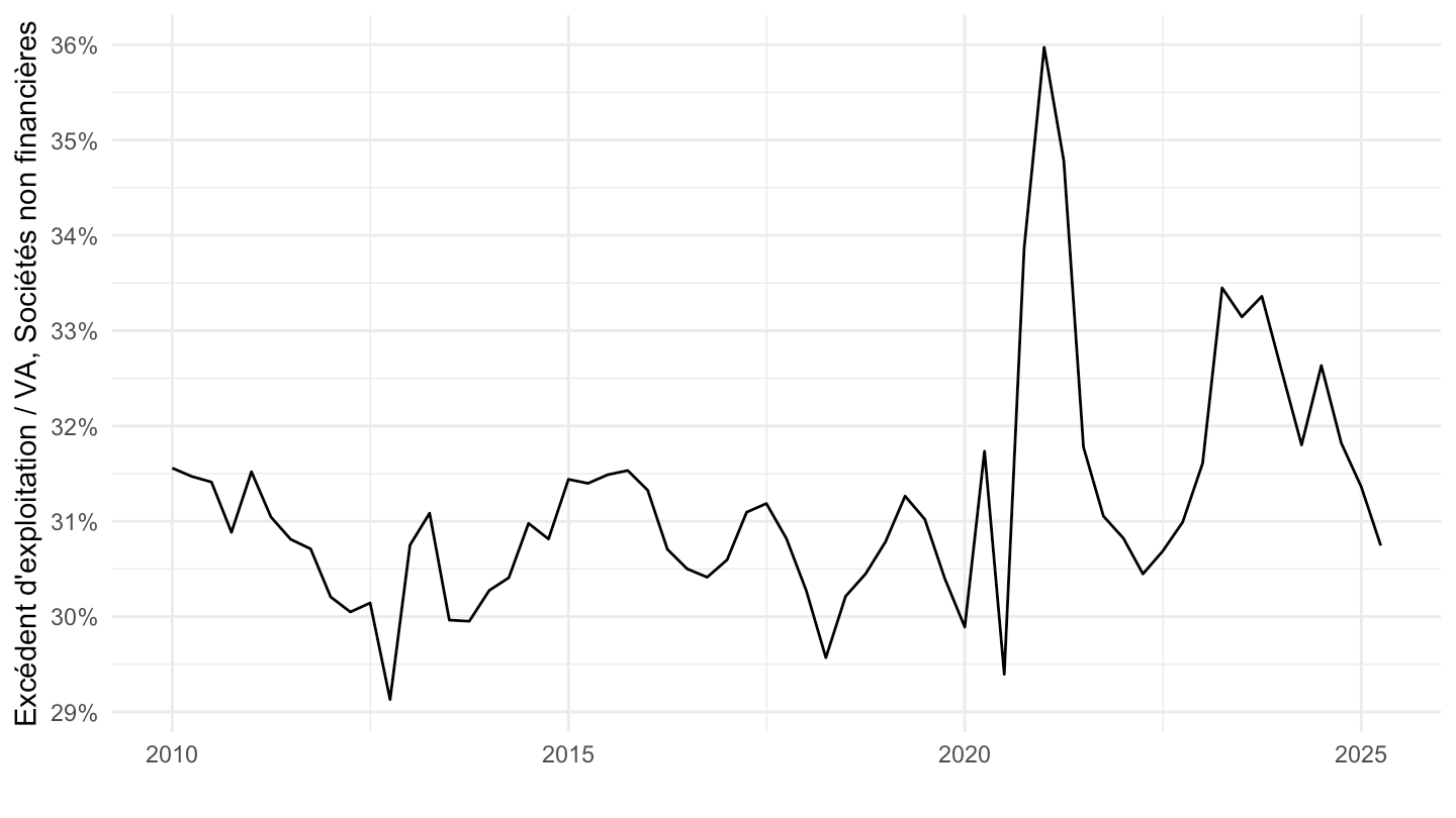
1 an
Code
`CNT-2020-CSI` %>%
  filter(`SECT-INST` == "S11",
         OPERATION %in% c("B2", "B1")) %>%

  quarter_to_date() %>%
  select(date, OBS_VALUE, OPERATION) %>%
  spread(OPERATION, OBS_VALUE) %>%
  mutate(obsValue = B2/B1,
         obsValue_mean = zoo::rollmean(obsValue, 4, fill = NA, align = "right")) %>%
  ggplot + geom_line(aes(x = date, y = obsValue_mean)) +
  theme_minimal() +  xlab("") + ylab("Excédent d'exploitation / VA, SNF, moyenne sur 1 an") +
  scale_x_date(breaks = as.Date(paste0(seq(1940, 2100, 5), "-01-01")),
               labels = date_format("%Y")) +
  scale_y_continuous(breaks = 0.01*seq(-2, 90, 1),
                     labels = scales::percent_format(accuracy = 1)) +
    geom_rect(data = data_frame(start = as.Date("2014-08-26"),
                                end = as.Date("2021-12-31")),
              aes(xmin = start, xmax = end, ymin = -Inf, ymax = +Inf),
              fill = viridis(4)[4], alpha = 0.2) +
  geom_vline(xintercept = as.Date("2014-08-26"), linetype = "dashed") +
  geom_vline(xintercept = as.Date("2017-05-07"), linetype = "dashed")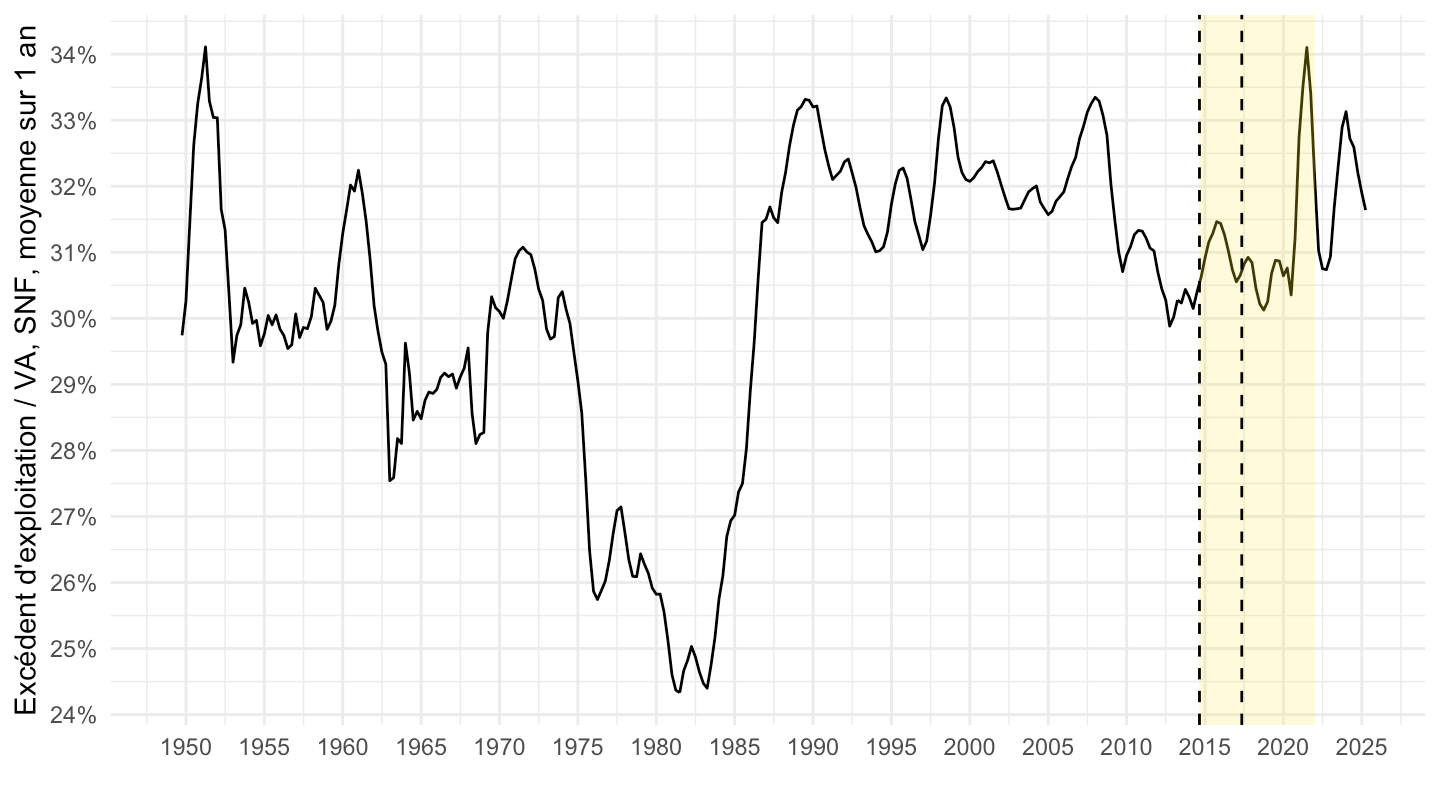
2 ans
Code
`CNT-2020-CSI` %>%
  filter(`SECT-INST` == "S11",
         OPERATION %in% c("B2", "B1")) %>%

  quarter_to_date() %>%
  select(date, OBS_VALUE, OPERATION) %>%
  spread(OPERATION, OBS_VALUE) %>%
  mutate(obsValue = B2/B1,
         obsValue_mean = zoo::rollmean(obsValue, 8, fill = NA, align = "right")) %>%
  ggplot + geom_line(aes(x = date, y = obsValue_mean)) +
  theme_minimal() +  xlab("") + ylab("Excédent d'exploitation / VA, SNF, moyenne sur 2 ans") +
  scale_x_date(breaks = as.Date(paste0(seq(1940, 2100, 5), "-01-01")),
               labels = date_format("%Y")) +
  scale_y_continuous(breaks = 0.01*seq(-2, 90, 1),
                     labels = scales::percent_format(accuracy = 1)) +
    geom_rect(data = data_frame(start = as.Date("2014-08-26"),
                                end = as.Date("2021-12-31")),
              aes(xmin = start, xmax = end, ymin = -Inf, ymax = +Inf),
              fill = viridis(4)[4], alpha = 0.2) +
  geom_vline(xintercept = as.Date("2014-08-26"), linetype = "dashed") +
  geom_vline(xintercept = as.Date("2017-05-07"), linetype = "dashed")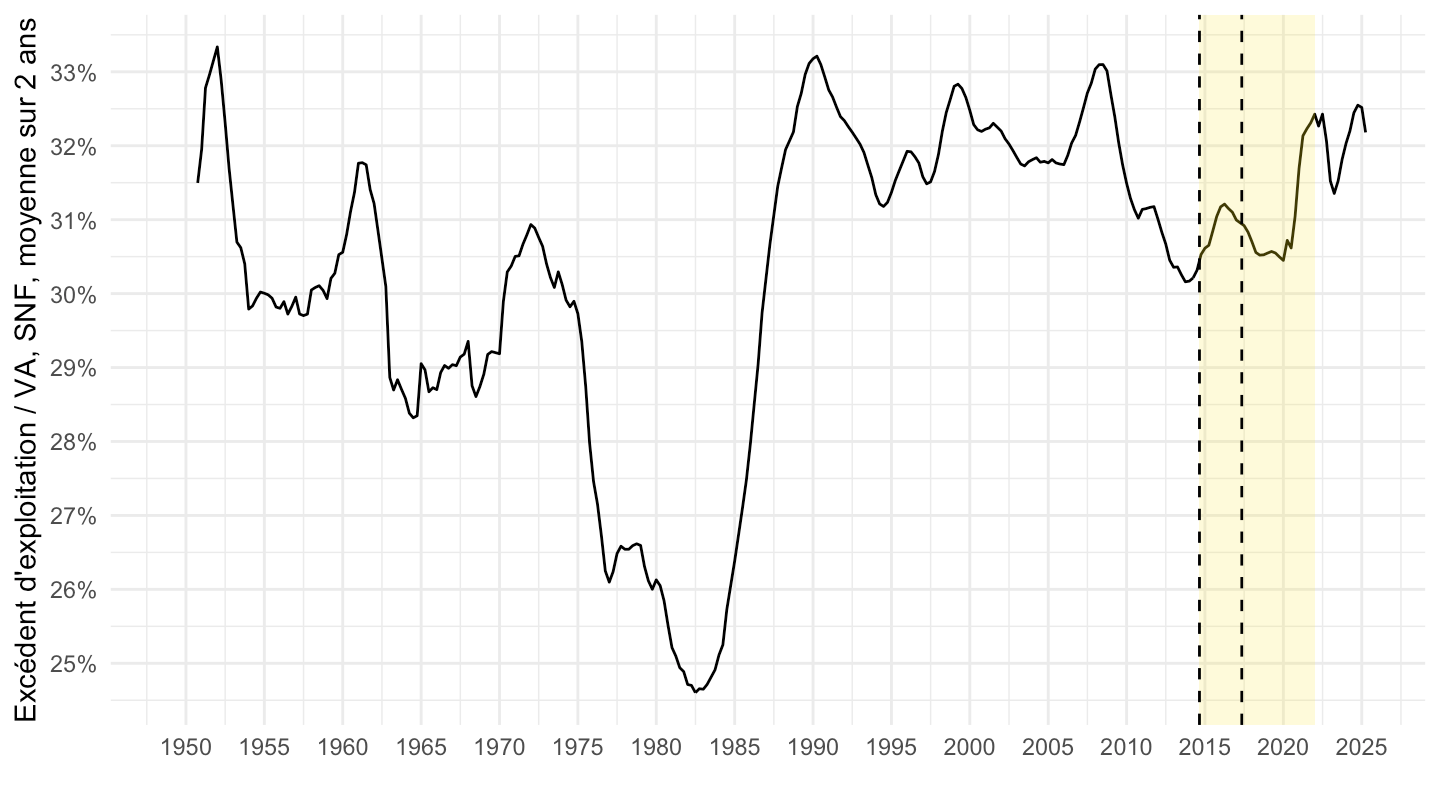
3 ans
Code
`CNT-2020-CSI` %>%
  filter(`SECT-INST` == "S11",
         OPERATION %in% c("B2", "B1")) %>%

  quarter_to_date() %>%
  select(date, OBS_VALUE, OPERATION) %>%
  spread(OPERATION, OBS_VALUE) %>%
  mutate(obsValue = B2/B1,
         obsValue_mean = zoo::rollmean(obsValue, 12, fill = NA, align = "right")) %>%
  ggplot + geom_line(aes(x = date, y = obsValue_mean)) +
  theme_minimal() +  xlab("") + ylab("Excédent d'exploitation / VA, SNF, moyenne sur 3 ans") +
  scale_x_date(breaks = as.Date(paste0(seq(1940, 2100, 5), "-01-01")),
               labels = date_format("%Y")) +
  scale_y_continuous(breaks = 0.01*seq(-2, 90, 1),
                     labels = scales::percent_format(accuracy = 1)) +
    geom_rect(data = data_frame(start = as.Date("2014-08-26"),
                                end = as.Date("2021-12-31")),
              aes(xmin = start, xmax = end, ymin = -Inf, ymax = +Inf),
              fill = viridis(4)[4], alpha = 0.2) +
  geom_vline(xintercept = as.Date("2014-08-26"), linetype = "dashed") +
  geom_vline(xintercept = as.Date("2017-05-07"), linetype = "dashed")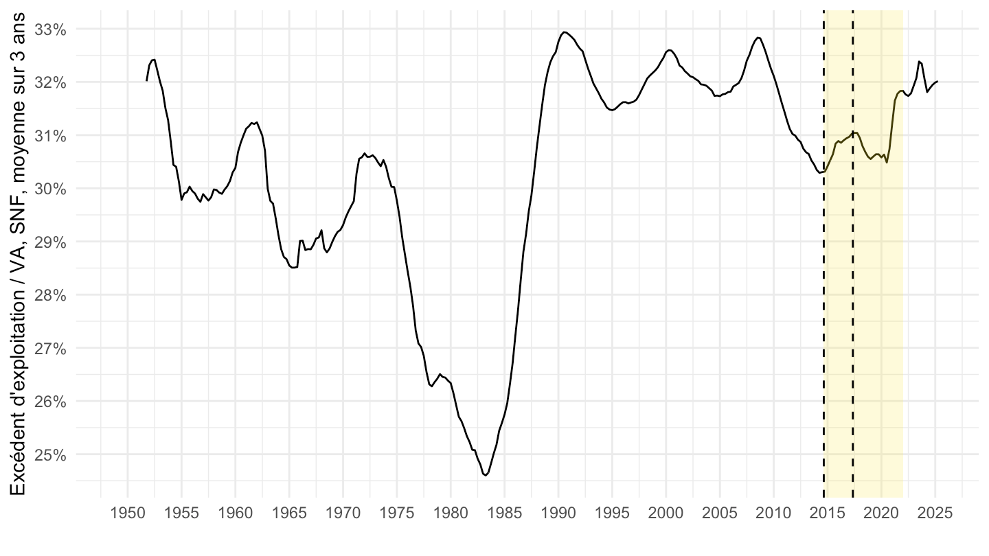
4 ans
Code
`CNT-2020-CSI` %>%
  filter(`SECT-INST` == "S11",
         OPERATION %in% c("B2", "B1")) %>%

  quarter_to_date() %>%
  select(date, OBS_VALUE, OPERATION) %>%
  spread(OPERATION, OBS_VALUE) %>%
  mutate(obsValue = B2/B1,
         obsValue_mean = zoo::rollmean(obsValue, 16, fill = NA, align = "right")) %>%
  ggplot + geom_line(aes(x = date, y = obsValue_mean)) +
  theme_minimal() +  xlab("") + ylab("Excédent d'exploitation / VA, SNF, moyenne sur 4 ans") +
  scale_x_date(breaks = as.Date(paste0(seq(1940, 2100, 5), "-01-01")),
               labels = date_format("%Y")) +
  scale_y_continuous(breaks = 0.01*seq(-2, 90, 1),
                     labels = scales::percent_format(accuracy = 1)) +
    geom_rect(data = data_frame(start = as.Date("2014-08-26"),
                                end = as.Date("2021-12-31")),
              aes(xmin = start, xmax = end, ymin = -Inf, ymax = +Inf),
              fill = viridis(4)[4], alpha = 0.2) +
  geom_vline(xintercept = as.Date("2014-08-26"), linetype = "dashed") +
  geom_vline(xintercept = as.Date("2017-05-07"), linetype = "dashed")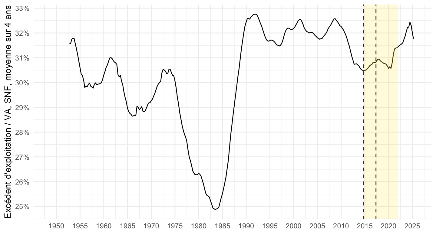
5 ans
Code
`CNT-2020-CSI` %>%
  filter(`SECT-INST` == "S11",
         OPERATION %in% c("B2", "B1")) %>%

  quarter_to_date() %>%
  select(date, OBS_VALUE, OPERATION) %>%
  spread(OPERATION, OBS_VALUE) %>%
  mutate(obsValue = B2/B1,
         obsValue_mean = zoo::rollmean(obsValue, 20, fill = NA, align = "right")) %>%
  ggplot + geom_line(aes(x = date, y = obsValue_mean)) +
  theme_minimal() +  xlab("") + ylab("Excédent d'exploitation / VA, SNF, moyenne sur 5 ans") +
  scale_x_date(breaks = as.Date(paste0(seq(1940, 2100, 5), "-01-01")),
               labels = date_format("%Y")) +
  scale_y_continuous(breaks = 0.01*seq(-2, 90, 1),
                     labels = scales::percent_format(accuracy = 1)) +
    geom_rect(data = data_frame(start = as.Date("2014-08-26"),
                                end = as.Date("2021-12-31")),
              aes(xmin = start, xmax = end, ymin = -Inf, ymax = +Inf),
              fill = viridis(4)[4], alpha = 0.2) +
  geom_vline(xintercept = as.Date("2014-08-26"), linetype = "dashed") +
  geom_vline(xintercept = as.Date("2017-05-07"), linetype = "dashed")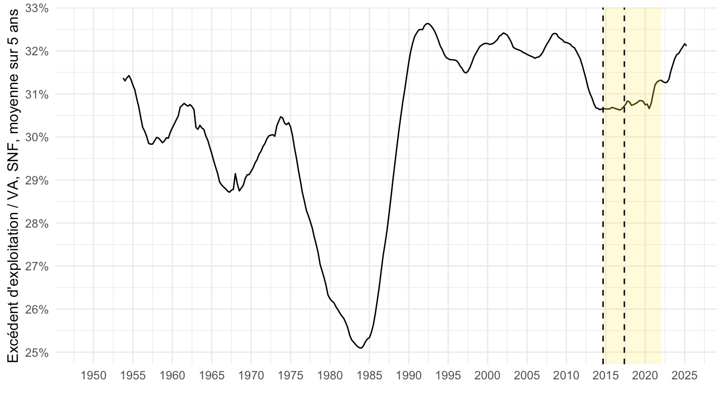
P51/B1G
Code
`CNT-2020-CSI` %>%
  filter(`SECT-INST` == "S11",
         OPERATION %in% c("P51", "B1")) %>%
  quarter_to_date() %>%
  select(date, OBS_VALUE, OPERATION) %>%
  spread(OPERATION, OBS_VALUE) %>%
  ggplot + geom_line(aes(x = date, y = P51/B1)) +
  theme_minimal() +  xlab("") + ylab("") +
  scale_x_date(breaks = as.Date(paste0(seq(1940, 2100, 5), "-01-01")),
               labels = date_format("%Y")) +
  scale_y_continuous(breaks = 0.01*seq(-2, 90, 1),
                     labels = scales::percent_format(accuracy = 1))
(D292+D39)/B1
All
Code
`CNT-2020-CSI` %>%
  filter(`SECT-INST` == "S11",
         OPERATION %in% c("D292", "B1", "D39")) %>%
  quarter_to_date() %>%
  select(date, OBS_VALUE, OPERATION) %>%
  spread(OPERATION, OBS_VALUE) %>%
  ggplot + geom_line(aes(x = date, y = (D292+D39)/B1)) +
  theme_minimal() +  xlab("") + ylab("Impôts - Subventions sur la production") +
  scale_x_date(breaks = as.Date(paste0(seq(1940, 2100, 5), "-01-01")),
               labels = date_format("%Y")) +
  scale_y_continuous(breaks = 0.01*seq(-2, 90, 1),
                     labels = scales::percent_format(accuracy = 1)) +
  geom_hline(yintercept = 0, linetype = "dashed", color = "red")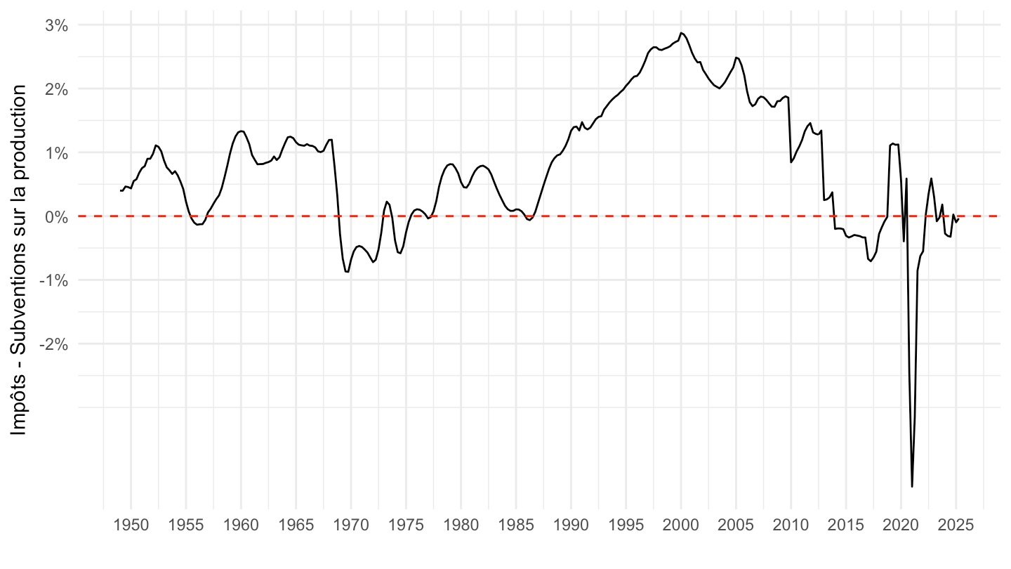
2000-
Code
`CNT-2020-CSI` %>%
  filter(`SECT-INST` == "S11",
         OPERATION %in% c("D292", "B1", "D39")) %>%
  quarter_to_date() %>%
  filter(date >= as.Date("2000-01-01")) %>%
  select(date, OBS_VALUE, OPERATION) %>%
  spread(OPERATION, OBS_VALUE) %>%
  ggplot + geom_line(aes(x = date, y = (D292+D39)/B1)) +
  theme_minimal() +  xlab("") + ylab("Impôts - Subventions sur la production") +
  scale_x_date(breaks = as.Date(paste0(seq(1940, 2100, 5), "-01-01")),
               labels = date_format("%Y")) +
  scale_y_continuous(breaks = 0.01*seq(-2, 90, 1),
                     labels = scales::percent_format(accuracy = 1)) +
  geom_hline(yintercept = 0, linetype = "dashed", color = "red")
Autres mesures
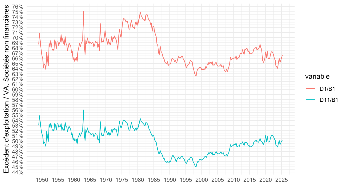
D1, D11: Brut et super brut
Code
`CNT-2020-CSI` %>%
  filter(`SECT-INST` == "S11",
         OPERATION %in% c("D1", "B1", "D11")) %>%

  quarter_to_date() %>%
  select(date, OBS_VALUE, OPERATION) %>%
  spread(OPERATION, OBS_VALUE) %>%
  transmute(date,
             `D1/B1` = D1/B1,
         `D11/B1` = D11/B1) %>%
  gather(variable, value, -date) %>%
  ggplot + geom_line(aes(x = date, y = value, color = variable)) +
  theme_minimal() +  xlab("") + ylab("Excédent d'exploitation / VA, Sociétés non financières") +
  scale_x_date(breaks = as.Date(paste0(seq(1940, 2100, 5), "-01-01")),
               labels = date_format("%Y")) +
  scale_y_continuous(breaks = 0.01*seq(-2, 90, 1),
                     labels = scales::percent_format(accuracy = 1))