| source | dataset | Title | .html | .rData |
|---|---|---|---|---|
| insee | CNT-2020-PIB-EQB-RF | Équilibre du produit intérieur brut | 2026-07-04 | 2026-06-20 |
Équilibre du produit intérieur brut
Données - INSEE
Info
Info
Données sur la macroéconomie en France
| source | dataset | Title | .html | .rData |
|---|---|---|---|---|
| bdf | CFT | Comptes Financiers Trimestriels | 2026-07-04 | 2025-03-09 |
| insee | CNA-2014-CONSO-SI | Dépenses de consommation finale par secteur institutionnel | 2026-07-04 | 2026-07-04 |
| insee | CNA-2014-CSI | Comptes des secteurs institutionnels | 2026-07-04 | 2026-07-04 |
| insee | CNA-2014-FBCF-BRANCHE | Formation brute de capital fixe (FBCF) par branche | 2026-07-04 | 2026-07-04 |
| insee | CNA-2014-FBCF-SI | Formation brute de capital fixe (FBCF) par secteur institutionnel | 2026-07-04 | 2026-07-04 |
| insee | CNA-2014-RDB | Revenu et pouvoir d’achat des ménages | 2026-07-04 | 2026-07-04 |
| insee | CNA-2020-CONSO-MEN | Consommation des ménages | 2026-07-04 | 2025-09-30 |
| insee | CNA-2020-PIB | Produit intérieur brut (PIB) et ses composantes | 2026-07-04 | 2025-05-28 |
| insee | CNT-2014-CB | Comptes des branches | 2026-07-04 | 2026-07-04 |
| insee | CNT-2014-CSI | Comptes de secteurs institutionnels | 2026-07-04 | 2026-07-04 |
| insee | CNT-2014-OPERATIONS | Opérations sur biens et services | 2026-07-04 | 2026-07-04 |
| insee | CNT-2014-PIB-EQB-RF | Équilibre du produit intérieur brut | 2026-07-04 | 2026-07-04 |
| insee | CONSO-MENAGES-2020 | Consommation des ménages en biens | 2026-07-04 | 2026-07-04 |
| insee | ICA-2015-IND-CONS | Indices de chiffre d'affaires dans l'industrie et la construction | 2026-07-04 | 2026-07-04 |
| insee | conso-mensuelle | Consommation de biens, données mensuelles | 2026-07-04 | 2023-07-04 |
| insee | t_1101 | 1.101 – Le produit intérieur brut et ses composantes à prix courants (En milliards d'euros) | 2026-07-04 | 2022-01-02 |
| insee | t_1102 | 1.102 – Le produit intérieur brut et ses composantes en volume aux prix de l'année précédente chaînés (En milliards d'euros 2014) | 2026-07-04 | 2020-10-30 |
| insee | t_1105 | 1.105 – Produit intérieur brut - les trois approches à prix courants (En milliards d'euros) - t_1105 | 2026-07-04 | 2020-10-30 |
LAST_UPDATE
Code
`CNT-2020-PIB-EQB-RF` %>%
  group_by(LAST_UPDATE) %>%
  summarise(Nobs = n()) %>%
  arrange(desc(LAST_UPDATE)) %>%
print_table_conditional()| LAST_UPDATE | Nobs |
|---|---|
| 2026-05-29 | 20493 |
| 2026-02-27 | 76 |
LAST_COMPILE
| LAST_COMPILE |
|---|
| 2026-07-04 |
Last
Code
`CNT-2020-PIB-EQB-RF` %>%
  filter(TIME_PERIOD == max(TIME_PERIOD)) %>%
  select(TIME_PERIOD, TITLE_FR, OBS_VALUE) %>%
  print_table_conditional()
Nobs
Code
`CNT-2020-PIB-EQB-RF` %>%
  left_join(OPERATION,  by = "OPERATION") %>%
  group_by(OPERATION, Operation, CNA_PRODUIT) %>%
  summarise(Nobs = n()) %>%
  arrange(-Nobs) %>%
  print_table_conditional()
TITLE_FR
Code
`CNT-2020-PIB-EQB-RF` %>%
  group_by(IDBANK, TITLE_FR) %>%
  summarise(Nobs = n()) %>%
  arrange(-Nobs) %>%
  print_table_conditional()
VALORISATION
Code
`CNT-2020-PIB-EQB-RF` %>%
  left_join(VALORISATION,  by = "VALORISATION") %>%
  group_by(VALORISATION, Valorisation) %>%
  summarise(Nobs = n()) %>%
  arrange(-Nobs) %>%
print_table_conditional()| VALORISATION | Valorisation | Nobs |
|---|---|---|
| L | Volumes aux prix de l'année précédente chaînés | 10990 |
| V | Valeurs aux prix courants | 7725 |
| SO | Sans objet | 1854 |
OPERATION
All
Code
`CNT-2020-PIB-EQB-RF` %>%
  left_join(OPERATION,  by = "OPERATION") %>%
  group_by(OPERATION, Operation) %>%
  summarise(Nobs = n()) %>%
  arrange(-Nobs) %>%
print_table_conditional()| OPERATION | Operation | Nobs |
|---|---|---|
| P3 | P3 - Dépense de consommation finale | 2462 |
| PIB | PIB - Produit intérieur brut | 1002 |
| DINTF | Demande intérieure totale finale | 922 |
| DINTFHS | Demande intérieure totale finale hors stocks | 922 |
| P31 | P31 - Dépense de consommation finale individuelle | 922 |
| P32 | P32 - Dépense de consommation finale collective | 922 |
| P4 | P4 - Consommation finale effective | 922 |
| P51 | P51 - Formation brute de capital fixe | 922 |
| P51B | P51B - FBCF des entreprises financières (y compris entreprises individuelles) | 922 |
| P51G | P51G - Formation brute de capital fixe | 922 |
| P51M | P51M - FBCF des ménages (hors entreprises individuelles) | 922 |
| P51P | P51P - FBCF des ISBLSM | 922 |
| P51S | P51S - FBCF des entreprises non financières (y compris entreprises individuelles) | 922 |
| P6 | P6 - Exportations de biens et services | 922 |
| P7 | P7 - Importations de biens et services | 922 |
| P54 | P54 - Stocks et acquisitions moins cession d'objets de valeur | 613 |
| SOLDE | SOLDE - Solde extérieur total | 613 |
| P52 | P52 - Variation de stocks | 494 |
| D11 | D11 - Salaires et traitements bruts | 309 |
| D121 | D121 - Cotisations sociales effectives à la charge des employeurs | 309 |
| D122 | D122 - Cotisations sociales imputées à la charge des employeurs | 309 |
| D211 | D211 - Impôts de type 'Taxe à la Valeur Ajoutée' (TVA) | 309 |
| D212 | D212 - Impôts sur les importations autres que la taxe à la valeur ajoutée | 309 |
| D214 | D214 - Autres impôts sur les produits | 309 |
| D291 | D291 - Impôts sur les salaires et la main-d'oeuvre | 309 |
| D292 | D292 - Impôts divers sur la production | 309 |
| D319 | D319 - Autres subventions sur les produits | 309 |
| D39 | D39 - Subventions d'exploitation | 309 |
| P53 | P53 - Acquisitions moins cession d'objets de valeur | 309 |
Volume
Code
`CNT-2020-PIB-EQB-RF` %>%
  filter(FREQ == "T",
         VALORISATION == "L",
         NATURE == "VALEUR_ABSOLUE",
         `SECT-INST` == "SO") %>%
  left_join(OPERATION,  by = "OPERATION") %>%
  group_by(OPERATION, Operation) %>%
  summarise(Nobs = n(),
            Last = last(OBS_VALUE)) %>%
  arrange(-Nobs) %>%
print_table_conditional()| OPERATION | Operation | Nobs | Last |
|---|---|---|---|
| DINTF | Demande intérieure totale finale | 309 | 70368.00 |
| DINTFHS | Demande intérieure totale finale hors stocks | 309 | 68437.00 |
| P3 | P3 - Dépense de consommation finale | 309 | 17988.00 |
| P31 | P31 - Dépense de consommation finale individuelle | 309 | 8703.00 |
| P32 | P32 - Dépense de consommation finale collective | 309 | 9353.00 |
| P4 | P4 - Consommation finale effective | 309 | 56141.00 |
| P6 | P6 - Exportations de biens et services | 309 | 3999.00 |
| P7 | P7 - Importations de biens et services | 309 | 3951.00 |
| PIB | PIB - Produit intérieur brut | 309 | 69933.00 |
| P52 | P52 - Variation de stocks | 185 | 0.54 |
Valeur
Code
`CNT-2020-PIB-EQB-RF` %>%
  filter(FREQ == "T",
         VALORISATION == "V",
         NATURE == "VALEUR_ABSOLUE",
         `SECT-INST` == "SO") %>%
  left_join(OPERATION,  by = "OPERATION") %>%
  group_by(OPERATION, Operation) %>%
  summarise(Nobs = n(),
            Last = last(OBS_VALUE)) %>%
  arrange(-Nobs) %>%
print_table_conditional()| OPERATION | Operation | Nobs | Last |
|---|---|---|---|
| D211 | D211 - Impôts de type 'Taxe à la Valeur Ajoutée' (TVA) | 309 | 231 |
| D212 | D212 - Impôts sur les importations autres que la taxe à la valeur ajoutée | 309 | 4 |
| D214 | D214 - Autres impôts sur les produits | 309 | 153 |
| D319 | D319 - Autres subventions sur les produits | 309 | -27 |
| DINTF | Demande intérieure totale finale | 309 | 3151 |
| DINTFHS | Demande intérieure totale finale hors stocks | 309 | 3030 |
| P3 | P3 - Dépense de consommation finale | 309 | 483 |
| P31 | P31 - Dépense de consommation finale individuelle | 309 | 243 |
| P32 | P32 - Dépense de consommation finale collective | 309 | 239 |
| P4 | P4 - Consommation finale effective | 309 | 2415 |
| P52 | P52 - Variation de stocks | 309 | 120 |
| P53 | P53 - Acquisitions moins cession d'objets de valeur | 309 | 2 |
| P54 | P54 - Stocks et acquisitions moins cession d'objets de valeur | 309 | 122 |
| P6 | P6 - Exportations de biens et services | 309 | 462 |
| P7 | P7 - Importations de biens et services | 309 | 431 |
| PIB | PIB - Produit intérieur brut | 309 | 3182 |
| SOLDE | SOLDE - Solde extérieur total | 309 | 31 |
NATURE
Code
`CNT-2020-PIB-EQB-RF` %>%
  left_join(NATURE, by = "NATURE") %>%
  group_by(NATURE, Nature) %>%
  summarise(Nobs = n()) %>%
  arrange(-Nobs) %>%
print_table_conditional()| NATURE | Nature | Nobs |
|---|---|---|
| VALEUR_ABSOLUE | Valeur absolue | 15017 |
| RATIO | Ratio | 5168 |
| TAUX | Taux | 384 |
FREQ
Code
`CNT-2020-PIB-EQB-RF` %>%
  left_join(FREQ, by = "FREQ") %>%
  group_by(FREQ, Freq) %>%
  summarise(Nobs = n()) %>%
  arrange(-Nobs) %>%
print_table_conditional()| FREQ | Freq | Nobs |
|---|---|---|
| T | NA | 20493 |
| A | Annual | 76 |
UNIT_MEASURE
Code
`CNT-2020-PIB-EQB-RF` %>%
  group_by(UNIT_MEASURE) %>%
  summarise(Nobs = n()) %>%
print_table_conditional()| UNIT_MEASURE | Nobs |
|---|---|
| EUROS | 14832 |
| POURCENT | 384 |
| SO | 5353 |
CNA_PRODUIT
Code
`CNT-2020-PIB-EQB-RF` %>%
  left_join(CNA_PRODUIT, by = "CNA_PRODUIT") %>%
  group_by(CNA_PRODUIT, Cna_produit) %>%
  summarise(Nobs = n()) %>%
  arrange(-Nobs) %>%
print_table_conditional()| CNA_PRODUIT | Cna_produit | Nobs |
|---|---|---|
| D-CNT | Ensemble des biens et services | 12051 |
| SO | Sans objet | 8518 |
TIME_PERIOD
Code
`CNT-2020-PIB-EQB-RF` %>%
  group_by(TIME_PERIOD) %>%
  summarise(Nobs = n()) %>%
  arrange(desc(TIME_PERIOD)) %>%
  print_table_conditional()
Last - 2022-Q1
Tous
Code
`CNT-2020-PIB-EQB-RF` %>%
  filter(TIME_PERIOD == "2022-Q1") %>%
  select_if(~ n_distinct(.) > 1) %>%
  select(-IDBANK, -TITLE_EN) %>%
  arrange(-OBS_VALUE) %>%
  print_table_conditional
% du PIB
Code
`CNT-2020-PIB-EQB-RF` %>%
  filter(FREQ == "T",
         VALORISATION == "V",
         TIME_PERIOD == "2022-Q1") %>%
  select_if(~ n_distinct(.) > 1) %>%
  select(-IDBANK, -TITLE_EN) %>%
  arrange(-OBS_VALUE) %>%
  mutate(`% of GDP` = round(100*OBS_VALUE/OBS_VALUE[OPERATION == "PIB"], 1)) %>%
print_table_conditional| SECT-INST | OPERATION | CNA_PRODUIT | TITLE_FR | OBS_VALUE | % of GDP |
|---|---|---|---|---|---|
| SO | DINTF | SO | Demande intérieure totale finale - Valeur aux prix courants - Série CVS-CJO | 659582 | 101.6 |
| SO | DINTFHS | SO | Demande intérieure totale finale hors stocks - Valeur aux prix courants - Série CVS-CJO | 657978 | 101.3 |
| SO | PIB | SO | Produit intérieur brut total - Valeur aux prix courants - Série CVS-CJO | 649295 | 100.0 |
| SO | P4 | D-CNT | Dépenses de consommation totales - Valeur aux prix courants - Série CVS-CJO | 507187 | 78.1 |
| S14 | P3 | D-CNT | Dépenses de consommation des ménages - Total - Valeur aux prix courants - Série CVS-CJO | 331893 | 51.1 |
| SO | P7 | D-CNT | Importations - Total - Valeur aux prix courants - Série CVS-CJO | 240446 | 37.0 |
| SO | P6 | D-CNT | Exportations - Total - Valeur aux prix courants - Série CVS-CJO | 230158 | 35.4 |
| SO | P3 | SO | Dépenses de consommation des APU - Total - Valeur aux prix courants - Série CVS-CJO | 160461 | 24.7 |
| S0 | P51 | D-CNT | FBCF de l'ensemble des secteurs institutionnels - Total - Valeur aux prix courants - Série CVS-CJO | 150790 | 23.2 |
| SO | P31 | D-CNT | Dépenses de consommation individualisable des APU - Total - Valeur aux prix courants - Série CVS-CJO | 104611 | 16.1 |
| S11 | P51S | D-CNT | Investissement des entreprises non financières - Total - Valeur aux prix courants - Série CVS-CJO | 78216 | 12.0 |
| SO | P32 | D-CNT | Dépenses de consommation collective des APU - Total - Valeur aux prix courants - Série CVS-CJO | 55850 | 8.6 |
| SO | D211 | D-CNT | TVA - Total - Valeur aux prix courants - Série CVS-CJO | 48215 | 7.4 |
| S14 | P51M | D-CNT | FBCF des ménages - Total - Valeur aux prix courants - Série CVS-CJO | 38055 | 5.9 |
| SO | D214 | D-CNT | Autres impôts sur les produits - Total - Valeur aux prix courants - Série CVS-CJO | 30013 | 4.6 |
| S13 | P51G | D-CNT | FBCF des administrations publiques - Total - Valeur aux prix courants - Série CVS-CJO | 26566 | 4.1 |
| S15 | P3 | D-CNT | Dépenses de consommation des ISBLSM - Total - Valeur aux prix courants - Série CVS-CJO | 14833 | 2.3 |
| S12 | P51B | D-CNT | FBCF des sociétés financières - Total - Valeur aux prix courants - Série CVS-CJO | 6583 | 1.0 |
| SO | P54 | D-CNT | Stocks et acquisitions moins cessions d'objets de valeur - Total - Valeur aux prix courants - Série CVS-CJO | 1604 | 0.2 |
| S15 | P51P | D-CNT | FBCF des ISBLSM - Total - Valeur aux prix courants - Série CVS-CJO | 1372 | 0.2 |
| SO | P52 | D-CNT | Variation des stocks - Total - Valeur aux prix courants - Série CVS-CJO | 1352 | 0.2 |
| SO | D212 | D-CNT | Impôts sur importations - Total - Valeur aux prix courants - Série CVS-CJO | 829 | 0.1 |
| SO | P53 | D-CNT | Acquisitions moins cessions d'objets de valeur - Total - Valeur aux prix courants - Série CVS-CJO | 253 | 0.0 |
| SO | D319 | D-CNT | Subventions - Total - Valeur aux prix courants - Série CVS-CJO | -5903 | -0.9 |
| SO | SOLDE | SO | Solde extérieur total - Valeur aux prix courants - Série CVS-CJO | -10287 | -1.6 |
Deflators
All
Code
`CNT-2020-PIB-EQB-RF` %>%
  filter(OPERATION %in% c("PIB", "P3", "P4"),
         VALORISATION %in% c("V", "L"),
         NATURE == "VALEUR_ABSOLUE") %>%
  select_if(~ n_distinct(.) > 1) %>%
  select(-IDBANK, -TITLE_EN) %>%
  rowwise() %>%
  mutate(date = TIME_PERIOD_to_date(TIME_PERIOD)) %>%
  arrange(desc(date)) %>%
  group_by(OPERATION, `SECT-INST`, date) %>%
  summarise(deflator = 100*OBS_VALUE[VALORISATION == "V"]/OBS_VALUE[VALORISATION == "L"]) %>%
  ungroup %>%
  left_join(OPERATION, by = "OPERATION") %>%
  left_join(`SECT-INST`, by = "SECT-INST") %>%
  mutate(variable = paste0(OPERATION, " - ", `Sect-Inst`)) %>%
  ggplot + geom_line(aes(x = date, y = deflator, color = variable)) +
  theme_minimal() + xlab("") + ylab("") +
  scale_x_date(breaks = seq(1920, 2100, 5) %>% paste0("-01-01") %>% as.Date,
               labels = date_format("%Y")) +
  scale_y_log10() +
  theme(legend.position = c(0.5, 0.8),
        legend.title = element_blank())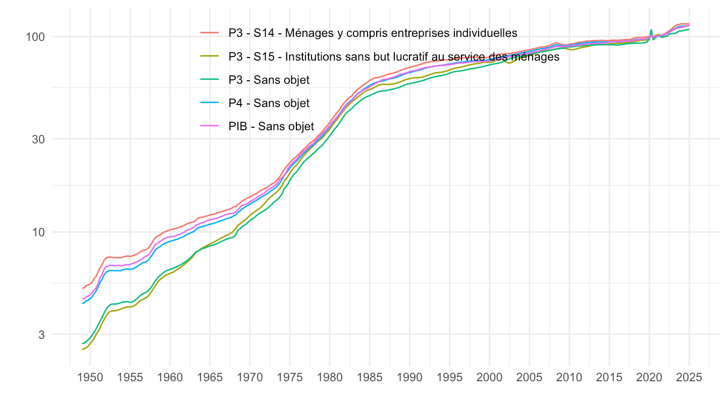
1999-
Code
`CNT-2020-PIB-EQB-RF` %>%
  filter(OPERATION %in% c("PIB", "P3", "P4"),
         VALORISATION %in% c("V", "L"),
         NATURE == "VALEUR_ABSOLUE") %>%
  select_if(~ n_distinct(.) > 1) %>%
  select(-IDBANK, -TITLE_EN) %>%
  rowwise() %>%
  mutate(date = TIME_PERIOD_to_date(TIME_PERIOD)) %>%
  arrange(desc(date)) %>%
  group_by(OPERATION, `SECT-INST`, date) %>%
  summarise(OBS_VALUE = 100*OBS_VALUE[VALORISATION == "V"]/OBS_VALUE[VALORISATION == "L"]) %>%
  ungroup %>%
  left_join(OPERATION, by = "OPERATION") %>%
  left_join(`SECT-INST`, by = "SECT-INST") %>%
  mutate(variable = paste0(OPERATION, " - ", `Sect-Inst`)) %>%
  filter(date >= as.Date("1999-01-01")) %>%

  group_by(variable) %>%
  mutate(OBS_VALUE = 100*OBS_VALUE/OBS_VALUE[1]) %>%
  ggplot + geom_line(aes(x = date, y = OBS_VALUE  , color = variable)) +
  theme_minimal() + xlab("") + ylab("") +
  scale_x_date(breaks = seq(1999, 2100, 5) %>% paste0("-01-01") %>% as.Date,
               labels = date_format("%Y")) +
  scale_y_log10(breaks = seq(100, 200, 5)) +
  theme(legend.position = c(0.5, 0.8),
        legend.title = element_blank())+
  geom_label_repel(data = . %>%
               filter(date == max(date)), aes(date, y = OBS_VALUE, label = round(OBS_VALUE, 1),color = variable))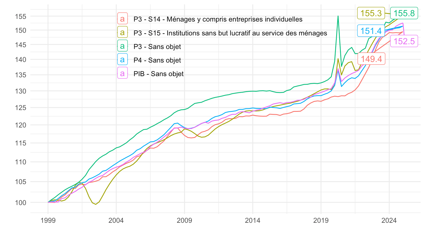
2014-
Code
`CNT-2020-PIB-EQB-RF` %>%
  filter(OPERATION %in% c("PIB", "P3", "P4"),
         VALORISATION %in% c("V", "L"),
         NATURE == "VALEUR_ABSOLUE") %>%
  select_if(~ n_distinct(.) > 1) %>%
  select(-IDBANK, -TITLE_EN) %>%
  rowwise() %>%
  mutate(date = TIME_PERIOD_to_date(TIME_PERIOD)) %>%
  arrange(desc(date)) %>%
  group_by(OPERATION, `SECT-INST`, date) %>%
  summarise(OBS_VALUE = 100*OBS_VALUE[VALORISATION == "V"]/OBS_VALUE[VALORISATION == "L"]) %>%
  ungroup %>%
  left_join(OPERATION, by = "OPERATION") %>%
  left_join(`SECT-INST`, by = "SECT-INST") %>%
  filter(date >= as.Date("2014-01-01")) %>%
  mutate(variable = paste0(OPERATION, " - ", `Sect-Inst`)) %>%
  group_by(variable) %>%
  mutate(OBS_VALUE = 100*OBS_VALUE/OBS_VALUE[1]) %>%
  ggplot + geom_line(aes(x = date, y = OBS_VALUE  , color = variable)) +
  theme_minimal() + xlab("") + ylab("") +
  scale_x_date(breaks = seq(1920, 2100, 1) %>% paste0("-01-01") %>% as.Date,
               labels = date_format("%Y")) +
  scale_y_log10() +
  theme(legend.position = c(0.5, 0.8),
        legend.title = element_blank())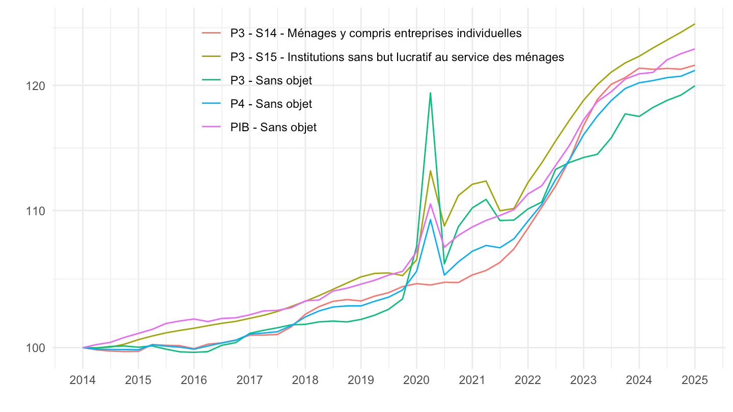
2019-
Code
`CNT-2020-PIB-EQB-RF` %>%
  filter(OPERATION %in% c("PIB", "P3", "P4"),
         VALORISATION %in% c("V", "L"),
         NATURE == "VALEUR_ABSOLUE") %>%
  select_if(~ n_distinct(.) > 1) %>%
  select(-IDBANK, -TITLE_EN) %>%
  rowwise() %>%
  mutate(date = TIME_PERIOD_to_date(TIME_PERIOD)) %>%
  arrange(desc(date)) %>%
  group_by(OPERATION, `SECT-INST`, date) %>%
  summarise(deflator = 100*OBS_VALUE[VALORISATION == "V"]/OBS_VALUE[VALORISATION == "L"]) %>%
  ungroup %>%
  left_join(OPERATION, by = "OPERATION") %>%
  left_join(`SECT-INST`, by = "SECT-INST") %>%
  filter(date >= as.Date("2019-01-01")) %>%
  mutate(variable = paste0(OPERATION, " - ", `Sect-Inst`)) %>%
  ggplot + geom_line(aes(x = date, y = deflator, color = variable)) +
  theme_minimal() + xlab("") + ylab("") +
  scale_x_date(breaks = seq(1920, 2100, 1) %>% paste0("-01-01") %>% as.Date,
               labels = date_format("%Y")) +
  scale_y_log10() +
  theme(legend.position = c(0.5, 0.8),
        legend.title = element_blank())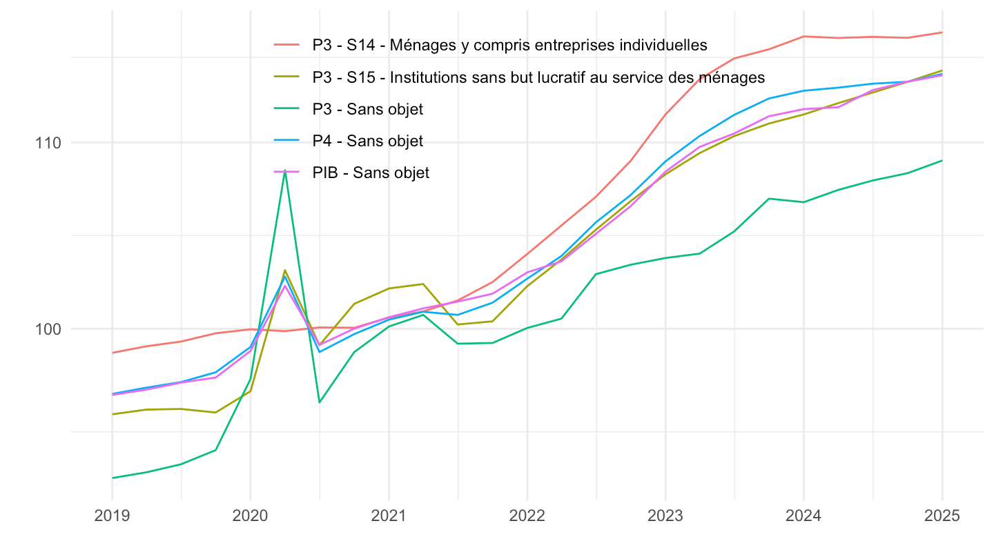
2017T2-
Code
`CNT-2020-PIB-EQB-RF` %>%
  filter(OPERATION %in% c("PIB", "P3", "P4"),
         VALORISATION %in% c("V", "L"),
         NATURE == "VALEUR_ABSOLUE") %>%
  select_if(~ n_distinct(.) > 1) %>%
  select(-IDBANK, -TITLE_EN) %>%
  rowwise() %>%
  mutate(date = TIME_PERIOD_to_date(TIME_PERIOD)) %>%
  arrange(desc(date)) %>%
  group_by(OPERATION, `SECT-INST`, date) %>%
  summarise(OBS_VALUE = 100*OBS_VALUE[VALORISATION == "V"]/OBS_VALUE[VALORISATION == "L"]) %>%
  ungroup %>%
  left_join(OPERATION, by = "OPERATION") %>%
  left_join(`SECT-INST`, by = "SECT-INST") %>%
  mutate(variable = paste0(OPERATION, " - ", `Sect-Inst`)) %>%
  filter(date >= as.Date("2017-04-01")) %>%

  group_by(variable) %>%
  mutate(OBS_VALUE = 100*OBS_VALUE/OBS_VALUE[1]) %>%
  ggplot + geom_line(aes(x = date, y = OBS_VALUE  , color = variable)) +
  theme_minimal() + xlab("") + ylab("") +
  scale_x_date(breaks = seq(1999, 2100, 1) %>% paste0("-01-01") %>% as.Date,
               labels = date_format("%Y")) +
  scale_y_log10(breaks = seq(100, 200, 5)) +
  theme(legend.position = c(0.5, 0.8),
        legend.title = element_blank())+
  geom_label_repel(data = . %>%
               filter(date == max(date)), aes(date, y = OBS_VALUE, label = round(OBS_VALUE, 1),color = variable))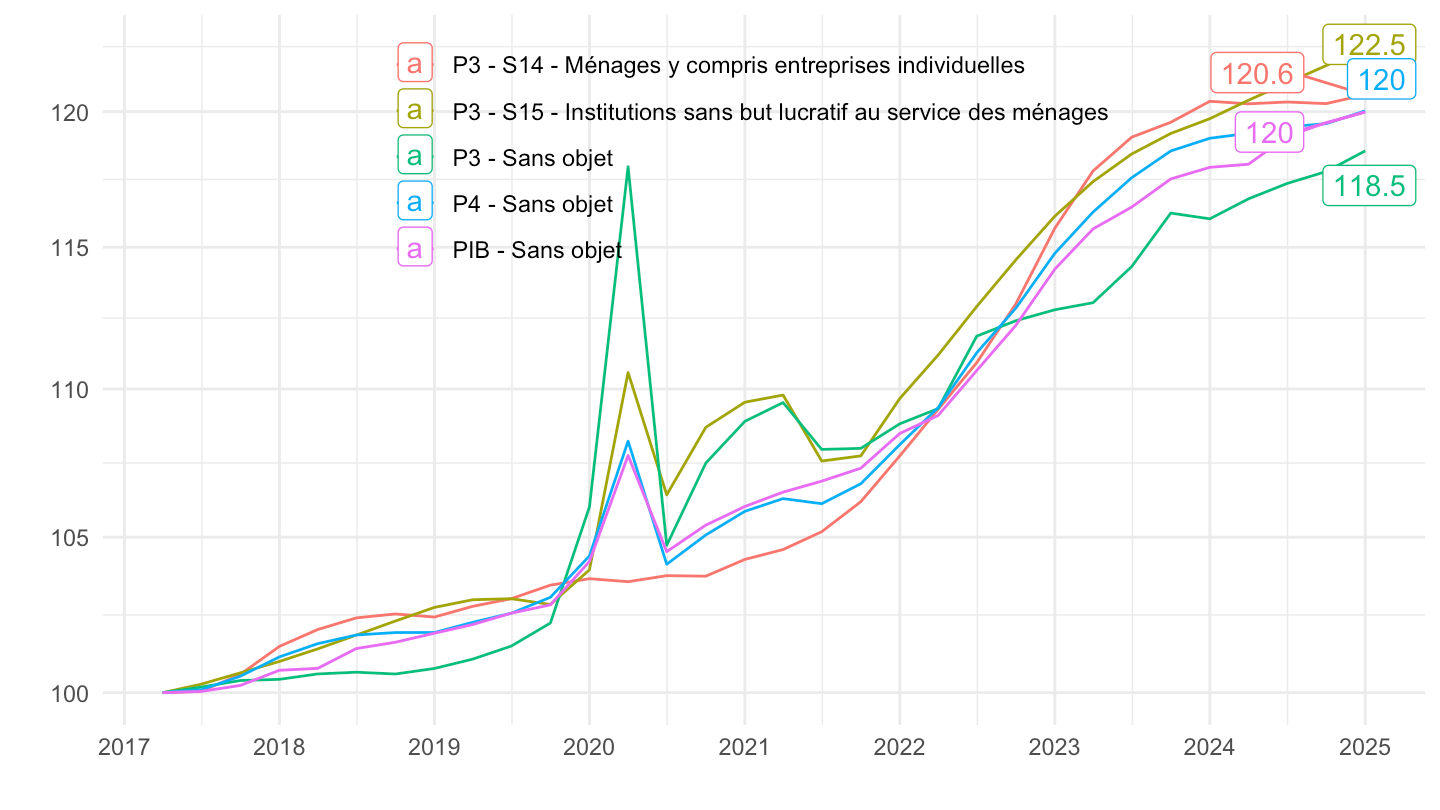
2019T4-
Code
`CNT-2020-PIB-EQB-RF` %>%
  filter(OPERATION %in% c("PIB", "P3", "P4"),
         VALORISATION %in% c("V", "L"),
         NATURE == "VALEUR_ABSOLUE") %>%
  select_if(~ n_distinct(.) > 1) %>%
  select(-IDBANK, -TITLE_EN) %>%
  rowwise() %>%
  mutate(date = TIME_PERIOD_to_date(TIME_PERIOD)) %>%
  arrange(desc(date)) %>%
  group_by(OPERATION, `SECT-INST`, date) %>%
  summarise(OBS_VALUE = 100*OBS_VALUE[VALORISATION == "V"]/OBS_VALUE[VALORISATION == "L"]) %>%
  ungroup %>%
  left_join(OPERATION, by = "OPERATION") %>%
  left_join(`SECT-INST`, by = "SECT-INST") %>%
  mutate(variable = paste0(OPERATION, " - ", `Sect-Inst`)) %>%
  filter(date >= as.Date("2019-10-01")) %>%

  group_by(variable) %>%
  mutate(OBS_VALUE = 100*OBS_VALUE/OBS_VALUE[1]) %>%
  ggplot + geom_line(aes(x = date, y = OBS_VALUE  , color = variable)) +
  theme_minimal() + xlab("") + ylab("") +
  scale_x_date(breaks = seq(1999, 2100, 1) %>% paste0("-01-01") %>% as.Date,
               labels = date_format("%Y")) +
  scale_y_log10(breaks = seq(100, 200, 5)) +
  theme(legend.position = c(0.5, 0.8),
        legend.title = element_blank())+
  geom_label_repel(data = . %>%
               filter(date == max(date)), aes(date, y = OBS_VALUE, label = round(OBS_VALUE, 1),color = variable))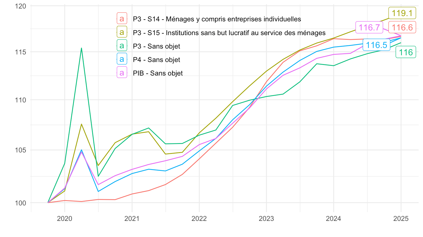
2020-
Code
`CNT-2020-PIB-EQB-RF` %>%
  filter(OPERATION %in% c("PIB", "P3", "P4"),
         VALORISATION %in% c("V", "L"),
         NATURE == "VALEUR_ABSOLUE") %>%
  select_if(~ n_distinct(.) > 1) %>%
  select(-IDBANK, -TITLE_EN) %>%
  rowwise() %>%
  mutate(date = TIME_PERIOD_to_date(TIME_PERIOD)) %>%
  arrange(desc(date)) %>%
  group_by(OPERATION, `SECT-INST`, date) %>%
  summarise(deflator = 100*OBS_VALUE[VALORISATION == "V"]/OBS_VALUE[VALORISATION == "L"]) %>%
  ungroup %>%
  left_join(OPERATION, by = "OPERATION") %>%
  left_join(`SECT-INST`, by = "SECT-INST") %>%
  filter(date >= as.Date("2020-01-01")) %>%
  mutate(variable = paste0(OPERATION, " - ", `Sect-Inst`)) %>%
  ggplot + geom_line(aes(x = date, y = deflator, color = variable)) +
  theme_minimal() + xlab("") + ylab("") +
  scale_x_date(breaks = seq(1920, 2100, 1) %>% paste0("-01-01") %>% as.Date,
               labels = date_format("%Y")) +
  scale_y_log10() +
  theme(legend.position = c(0.5, 0.8),
        legend.title = element_blank())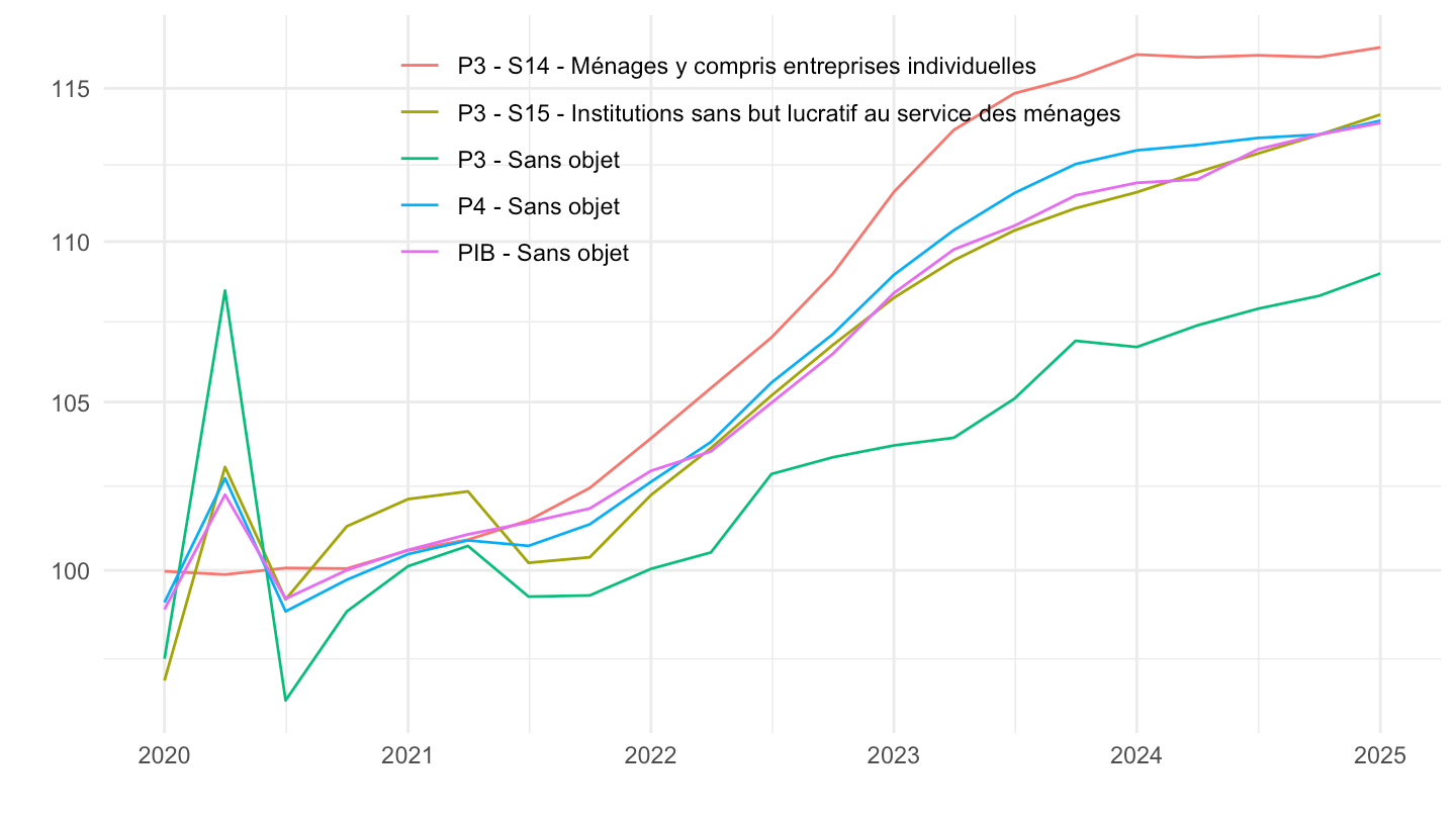
2021-
Code
`CNT-2020-PIB-EQB-RF` %>%
  filter(OPERATION %in% c("PIB", "P3", "P4"),
         VALORISATION %in% c("V", "L"),
         NATURE == "VALEUR_ABSOLUE") %>%
  select_if(~ n_distinct(.) > 1) %>%
  select(-IDBANK, -TITLE_EN) %>%
  rowwise() %>%
  mutate(date = TIME_PERIOD_to_date(TIME_PERIOD)) %>%
  arrange(desc(date)) %>%
  group_by(OPERATION, `SECT-INST`, date) %>%
  summarise(deflator = 100*OBS_VALUE[VALORISATION == "V"]/OBS_VALUE[VALORISATION == "L"]) %>%
  ungroup %>%
  left_join(OPERATION, by = "OPERATION") %>%
  left_join(`SECT-INST`, by = "SECT-INST") %>%
  filter(date >= as.Date("2021-01-01")) %>%
  mutate(variable = paste0(OPERATION, " - ", `Sect-Inst`)) %>%
  group_by(OPERATION, `SECT-INST`) %>%
  mutate(deflator = 100*deflator/deflator[1]) %>%
  ggplot + geom_line(aes(x = date, y = deflator, color = variable)) +
  theme_minimal() + xlab("") + ylab("") +
  scale_x_date(breaks = seq(1920, 2100, 1) %>% paste0("-01-01") %>% as.Date,
               labels = date_format("%Y")) +
  scale_y_log10() +
  theme(legend.position = c(0.5, 0.8),
        legend.title = element_blank())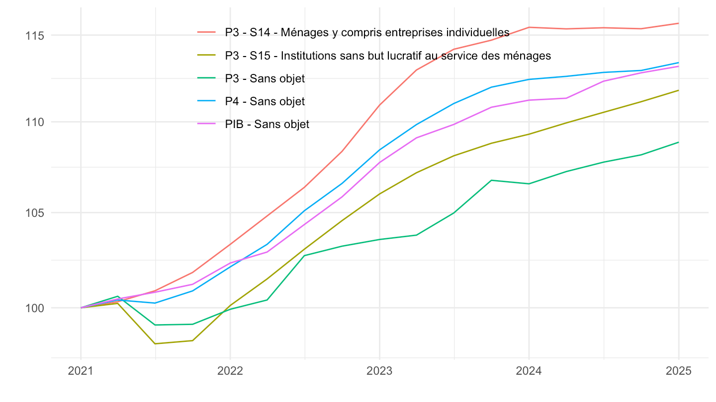
Agrégats
consommation nominale
Code
`CNT-2020-PIB-EQB-RF` %>%
  filter(FREQ == "T",
         VALORISATION == "V",
         OPERATION %in% c("P3", "PIB")) %>%
  quarter_to_date %>%
  filter(date >= as.Date("2021-10-01")) %>%
  group_by(OPERATION, `SECT-INST`) %>%
  arrange(date) %>%
  mutate(OBS_VALUE = OBS_VALUE/OBS_VALUE[1]) %>%
  mutate(TITLE_FR = gsub("- Valeur aux prix courants - Série CVS-CJO", "", TITLE_FR)) %>%
  ggplot() + ylab("% du PIB") + xlab("") + theme_minimal() +
  geom_line(aes(x = date, y = OBS_VALUE, color = TITLE_FR)) +

  scale_x_date(breaks = seq(1920, 2100, 1) %>% paste0("-01-01") %>% as.Date,
               labels = date_format("%Y")) +
  theme(legend.position = c(0.25, 0.4),
        legend.title = element_blank()) +
  scale_y_continuous(breaks = 0.01*seq(0, 300, 5),
                     labels = percent_format(accuracy = 1))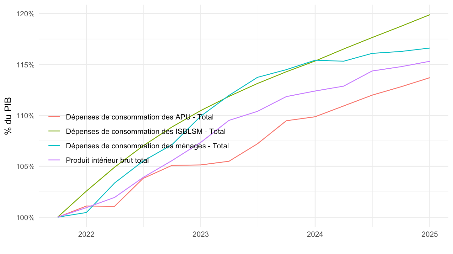
Consommation: P4, P3
All
Code
`CNT-2020-PIB-EQB-RF` %>%
  filter(FREQ == "T",
         VALORISATION == "V",
         OPERATION %in% c("P4", "P3", "PIB")) %>%
  quarter_to_date %>%
  group_by(date) %>%
  mutate(OBS_VALUE = OBS_VALUE/OBS_VALUE[OPERATION == "PIB"]) %>%
  filter(OPERATION != "PIB") %>%
  mutate(TITLE_FR = gsub("- Valeur aux prix courants - Série CVS-CJO", "", TITLE_FR)) %>%
  ggplot() + ylab("% du PIB") + xlab("") + theme_minimal() +
  geom_line(aes(x = date, y = OBS_VALUE, color = TITLE_FR)) +

  scale_x_date(breaks = seq(1920, 2100, 5) %>% paste0("-01-01") %>% as.Date,
               labels = date_format("%Y")) +
  theme(legend.position = c(0.25, 0.4),
        legend.title = element_blank()) +
  scale_y_continuous(breaks = 0.01*seq(0, 300, 5),
                     labels = percent_format(accuracy = 1))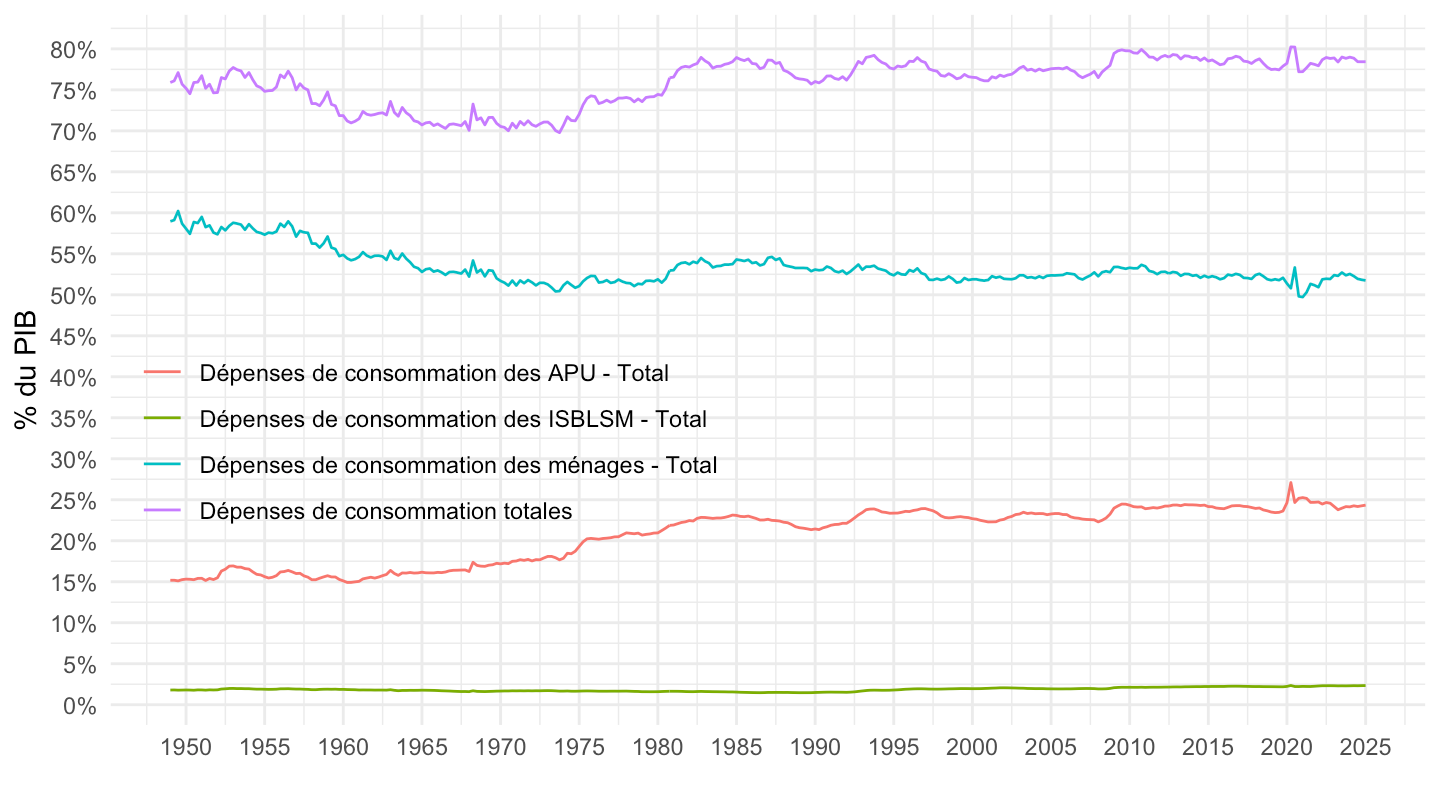
1980-
Code
`CNT-2020-PIB-EQB-RF` %>%
  filter(FREQ == "T",
         VALORISATION == "V",
         OPERATION %in% c("P4", "P3", "PIB")) %>%
  quarter_to_date %>%
  group_by(date) %>%
  mutate(OBS_VALUE = OBS_VALUE/OBS_VALUE[OPERATION == "PIB"]) %>%
  filter(OPERATION != "PIB") %>%
  mutate(TITLE_FR = gsub("- Valeur aux prix courants - Série CVS-CJO", "", TITLE_FR)) %>%
  filter(date >= as.Date("1980-01-01")) %>%
  ggplot() + ylab("% du PIB") + xlab("") + theme_minimal() +
  geom_line(aes(x = date, y = OBS_VALUE, color = TITLE_FR)) +

  scale_x_date(breaks = seq(1920, 2100, 5) %>% paste0("-01-01") %>% as.Date,
               labels = date_format("%Y")) +
  theme(legend.position = c(0.25, 0.4),
        legend.title = element_blank()) +
  scale_y_continuous(breaks = 0.01*seq(0, 300, 5),
                     labels = percent_format(accuracy = 1))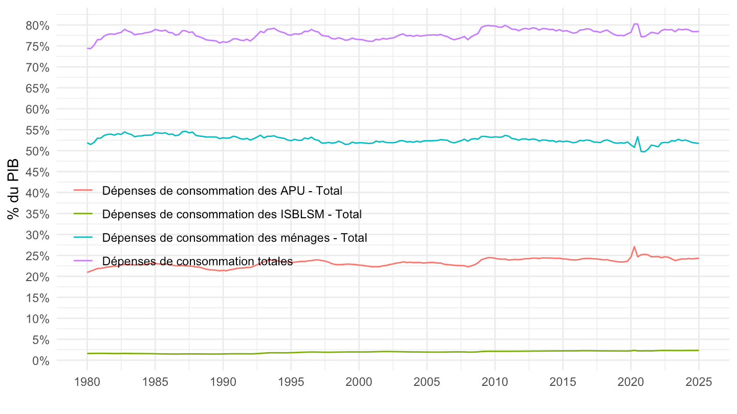
1995-
Code
`CNT-2020-PIB-EQB-RF` %>%
  filter(FREQ == "T",
         VALORISATION == "V",
         OPERATION %in% c("P4", "P3", "PIB")) %>%
  quarter_to_date %>%
  group_by(date) %>%
  mutate(OBS_VALUE = OBS_VALUE/OBS_VALUE[OPERATION == "PIB"]) %>%
  filter(OPERATION != "PIB") %>%
  mutate(TITLE_FR = gsub("- Valeur aux prix courants - Série CVS-CJO", "", TITLE_FR)) %>%
  filter(date >= as.Date("1995-01-01")) %>%
  ggplot() + ylab("% du PIB") + xlab("") + theme_minimal() +
  geom_line(aes(x = date, y = OBS_VALUE, color = TITLE_FR)) +

  scale_x_date(breaks = seq(1920, 2100, 5) %>% paste0("-01-01") %>% as.Date,
               labels = date_format("%Y")) +
  theme(legend.position = c(0.25, 0.4),
        legend.title = element_blank()) +
  scale_y_continuous(breaks = 0.01*seq(0, 300, 5),
                     labels = percent_format(accuracy = 1))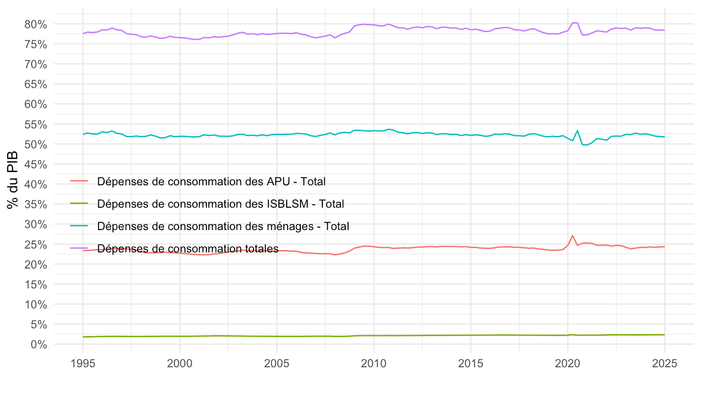
2000-
Code
`CNT-2020-PIB-EQB-RF` %>%
  filter(FREQ == "T",
         VALORISATION == "V",
         OPERATION %in% c("P4", "P3", "PIB")) %>%
  quarter_to_date %>%
  group_by(date) %>%
  mutate(OBS_VALUE = OBS_VALUE/OBS_VALUE[OPERATION == "PIB"]) %>%
  filter(OPERATION != "PIB") %>%
  mutate(TITLE_FR = gsub("- Valeur aux prix courants - Série CVS-CJO", "", TITLE_FR)) %>%
  filter(date >= as.Date("2000-01-01")) %>%
  ggplot() + ylab("% du PIB") + xlab("") + theme_minimal() +
  geom_line(aes(x = date, y = OBS_VALUE, color = TITLE_FR)) +

  scale_x_date(breaks = seq(1920, 2100, 5) %>% paste0("-01-01") %>% as.Date,
               labels = date_format("%Y")) +
  theme(legend.position = c(0.25, 0.4),
        legend.title = element_blank()) +
  scale_y_continuous(breaks = 0.01*seq(0, 300, 5),
                     labels = percent_format(accuracy = 1))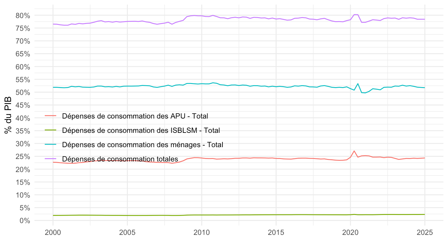
All
Code
`CNT-2020-PIB-EQB-RF` %>%
  filter(FREQ == "T",
         VALORISATION == "V",
         OPERATION %in% c("P31", "P32", "PIB")) %>%
  quarter_to_date %>%
  group_by(date) %>%
  mutate(OBS_VALUE = OBS_VALUE/OBS_VALUE[OPERATION == "PIB"]) %>%
  filter(OPERATION != "PIB") %>%
  mutate(TITLE_FR = gsub("- Valeur aux prix courants - Série CVS-CJO", "", TITLE_FR)) %>%
  ggplot() + ylab("% du PIB") + xlab("") + theme_minimal() +
  geom_line(aes(x = date, y = OBS_VALUE, color = TITLE_FR)) +

  scale_x_date(breaks = seq(1920, 2100, 5) %>% paste0("-01-01") %>% as.Date,
               labels = date_format("%Y")) +
  theme(legend.position = c(0.3, 0.85),
        legend.title = element_blank()) +
  scale_y_continuous(breaks = 0.01*seq(0, 300, 1),
                     labels = percent_format(accuracy = 1))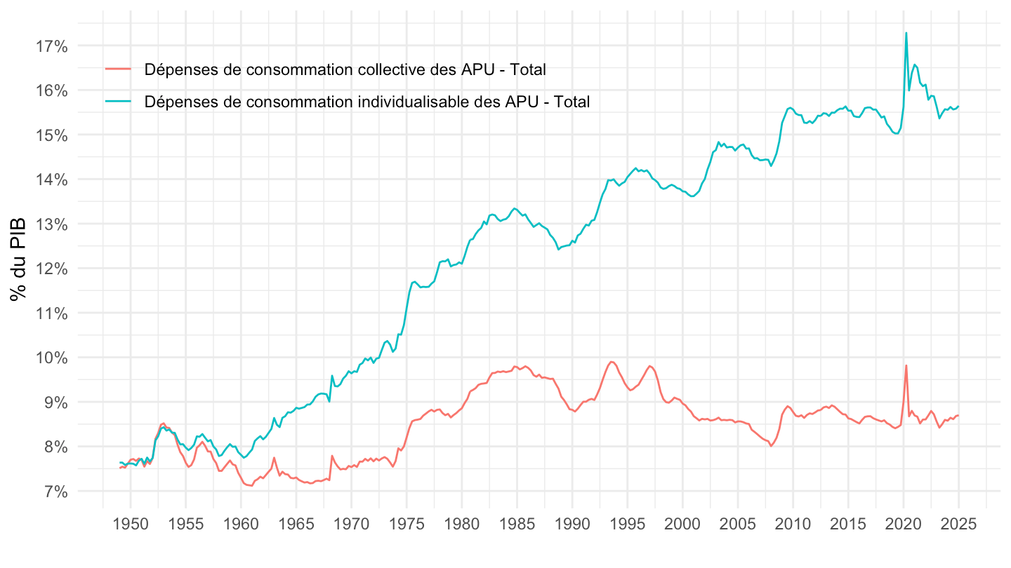
1980-
Code
`CNT-2020-PIB-EQB-RF` %>%
  filter(FREQ == "T",
         VALORISATION == "V",
         OPERATION %in% c("P31", "P32", "PIB")) %>%
  quarter_to_date %>%
  group_by(date) %>%
  mutate(OBS_VALUE = OBS_VALUE/OBS_VALUE[OPERATION == "PIB"]) %>%
  filter(OPERATION != "PIB") %>%
  mutate(TITLE_FR = gsub("- Valeur aux prix courants - Série CVS-CJO", "", TITLE_FR)) %>%
  filter(date >= as.Date("1980-01-01")) %>%
  ggplot() + ylab("% du PIB") + xlab("") + theme_minimal() +
  geom_line(aes(x = date, y = OBS_VALUE, color = TITLE_FR)) +

  scale_x_date(breaks = seq(1920, 2100, 5) %>% paste0("-01-01") %>% as.Date,
               labels = date_format("%Y")) +
  theme(legend.position = c(0.3, 0.85),
        legend.title = element_blank()) +
  scale_y_continuous(breaks = 0.01*seq(0, 300, 1),
                     labels = percent_format(accuracy = 1))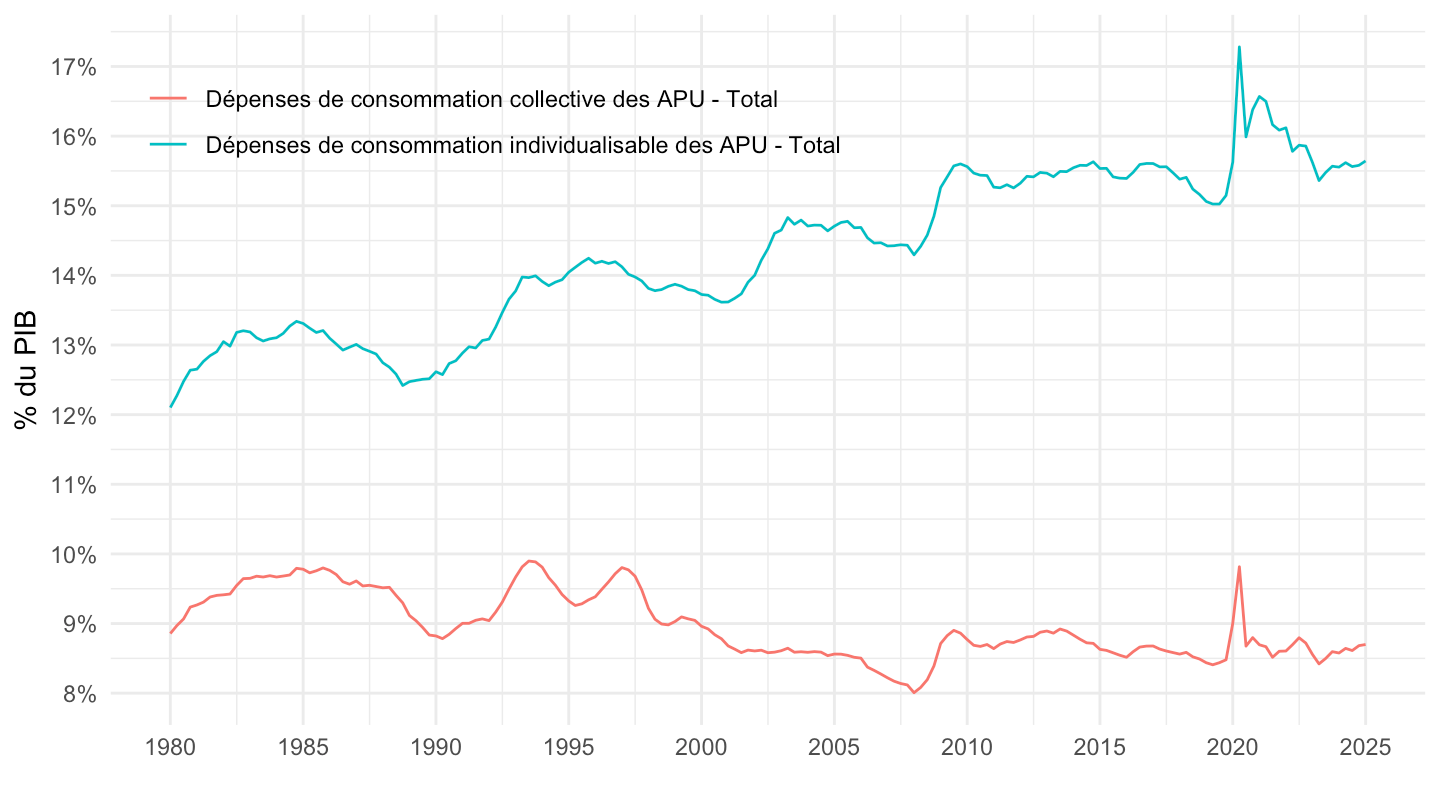
1995-
Code
`CNT-2020-PIB-EQB-RF` %>%
  filter(FREQ == "T",
         VALORISATION == "V",
         OPERATION %in% c("P31", "P32", "PIB")) %>%
  quarter_to_date %>%
  group_by(date) %>%
  mutate(OBS_VALUE = OBS_VALUE/OBS_VALUE[OPERATION == "PIB"]) %>%
  filter(OPERATION != "PIB") %>%
  mutate(TITLE_FR = gsub("- Valeur aux prix courants - Série CVS-CJO", "", TITLE_FR)) %>%
  filter(date >= as.Date("1995-01-01")) %>%
  ggplot() + ylab("% du PIB") + xlab("") + theme_minimal() +
  geom_line(aes(x = date, y = OBS_VALUE, color = TITLE_FR)) +

  scale_x_date(breaks = seq(1920, 2100, 5) %>% paste0("-01-01") %>% as.Date,
               labels = date_format("%Y")) +
  theme(legend.position = c(0.3, 0.85),
        legend.title = element_blank()) +
  scale_y_continuous(breaks = 0.01*seq(0, 300, 1),
                     labels = percent_format(accuracy = 1))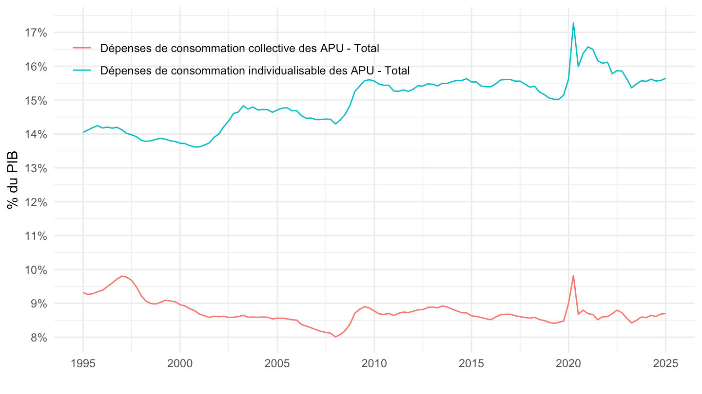
Exports, Imports
All
Code
`CNT-2020-PIB-EQB-RF` %>%
  filter(FREQ == "T",
         VALORISATION == "V",
         OPERATION %in% c("P6", "P7", "PIB")) %>%
  quarter_to_date %>%
  group_by(date) %>%
  mutate(OBS_VALUE = OBS_VALUE/OBS_VALUE[OPERATION == "PIB"]) %>%
  filter(OPERATION != "PIB") %>%
  mutate(TITLE_FR = gsub("- Valeur aux prix courants - Série CVS-CJO", "", TITLE_FR)) %>%
  ggplot() + ylab("% du PIB") + xlab("") + theme_minimal() +
  geom_line(aes(x = date, y = OBS_VALUE, color = TITLE_FR)) +

  scale_x_date(breaks = seq(1920, 2100, 5) %>% paste0("-01-01") %>% as.Date,
               labels = date_format("%Y")) +
  theme(legend.position = c(0.3, 0.85),
        legend.title = element_blank()) +
  scale_y_continuous(breaks = 0.01*seq(0, 300, 2),
                     labels = percent_format(accuracy = 1))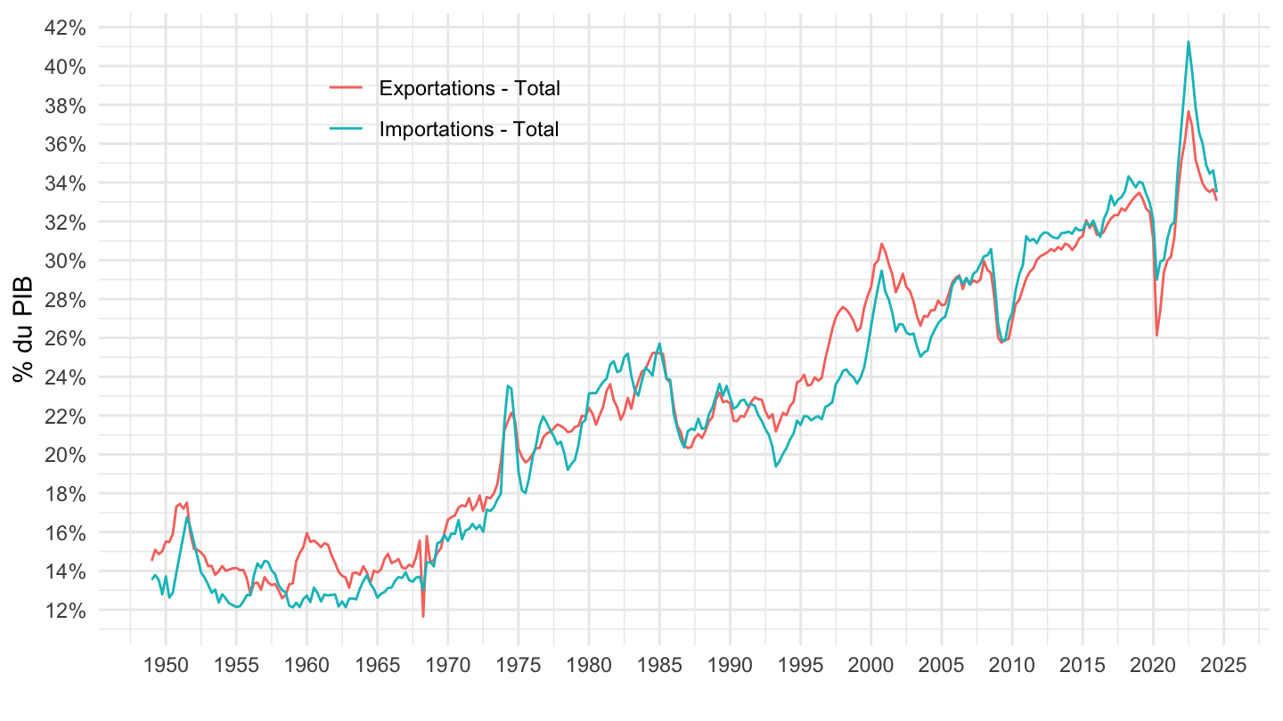
1980-
Code
`CNT-2020-PIB-EQB-RF` %>%
  filter(FREQ == "T",
         VALORISATION == "V",
         OPERATION %in% c("P6", "P7", "PIB")) %>%
  quarter_to_date %>%
  group_by(date) %>%
  mutate(OBS_VALUE = OBS_VALUE/OBS_VALUE[OPERATION == "PIB"]) %>%
  filter(OPERATION != "PIB") %>%
  mutate(TITLE_FR = gsub("- Valeur aux prix courants - Série CVS-CJO", "", TITLE_FR)) %>%
  filter(date >= as.Date("1980-01-01")) %>%
  ggplot() + ylab("% du PIB") + xlab("") + theme_minimal() +
  geom_line(aes(x = date, y = OBS_VALUE, color = TITLE_FR)) +

  scale_x_date(breaks = seq(1920, 2100, 5) %>% paste0("-01-01") %>% as.Date,
               labels = date_format("%Y")) +
  theme(legend.position = c(0.3, 0.85),
        legend.title = element_blank()) +
  scale_y_continuous(breaks = 0.01*seq(0, 300, 2),
                     labels = percent_format(accuracy = 1))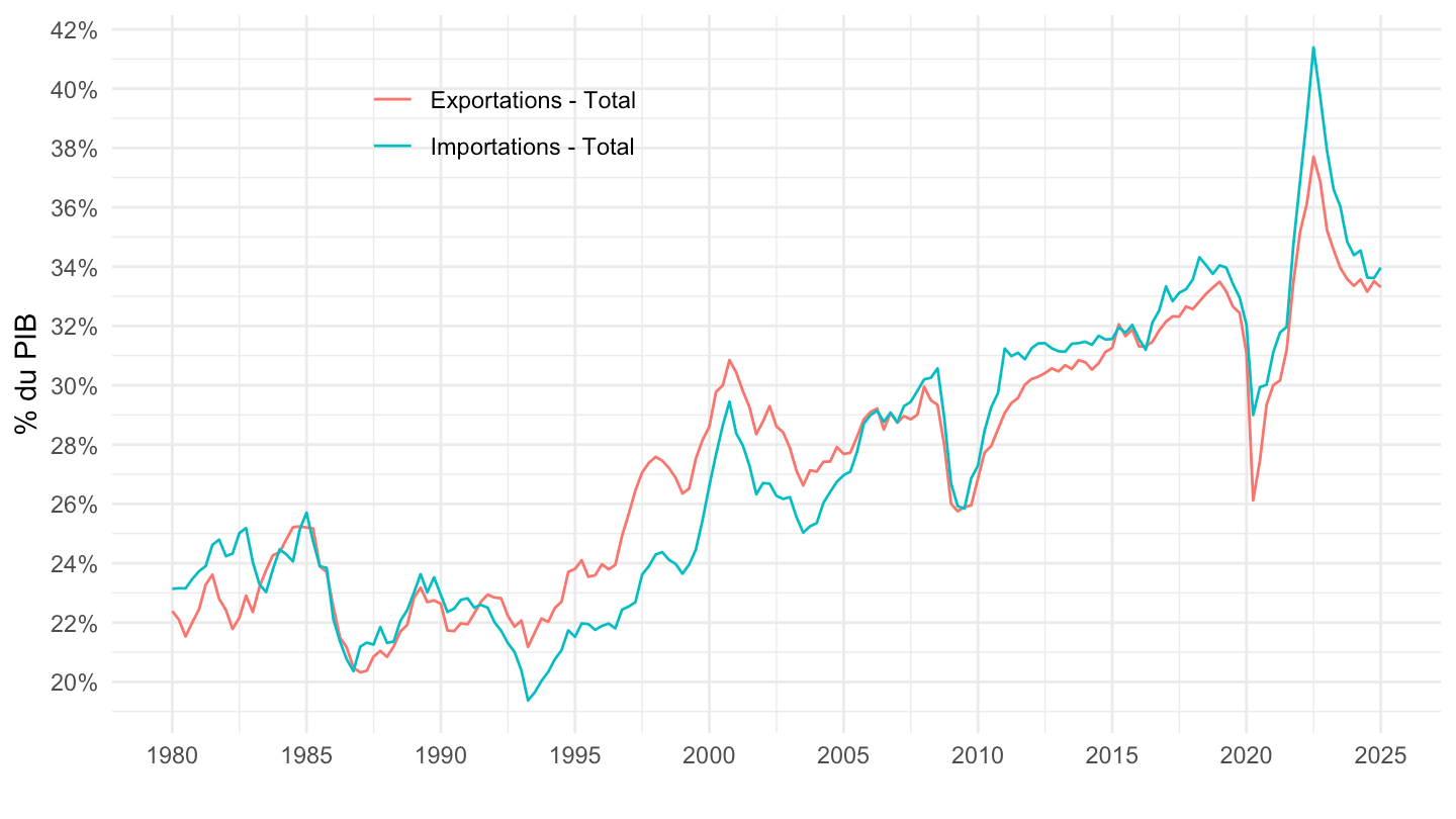
1995-
Code
`CNT-2020-PIB-EQB-RF` %>%
  filter(FREQ == "T",
         VALORISATION == "V",
         OPERATION %in% c("P6", "P7", "PIB")) %>%
  quarter_to_date %>%
  group_by(date) %>%
  mutate(OBS_VALUE = OBS_VALUE/OBS_VALUE[OPERATION == "PIB"]) %>%
  filter(OPERATION != "PIB") %>%
  mutate(TITLE_FR = gsub("- Valeur aux prix courants - Série CVS-CJO", "", TITLE_FR)) %>%
  filter(date >= as.Date("1995-01-01")) %>%
  ggplot() + ylab("% du PIB") + xlab("") + theme_minimal() +
  geom_line(aes(x = date, y = OBS_VALUE, color = TITLE_FR)) +

  scale_x_date(breaks = seq(1920, 2100, 5) %>% paste0("-01-01") %>% as.Date,
               labels = date_format("%Y")) +
  theme(legend.position = c(0.3, 0.85),
        legend.title = element_blank()) +
  scale_y_continuous(breaks = 0.01*seq(0, 300, 2),
                     labels = percent_format(accuracy = 1))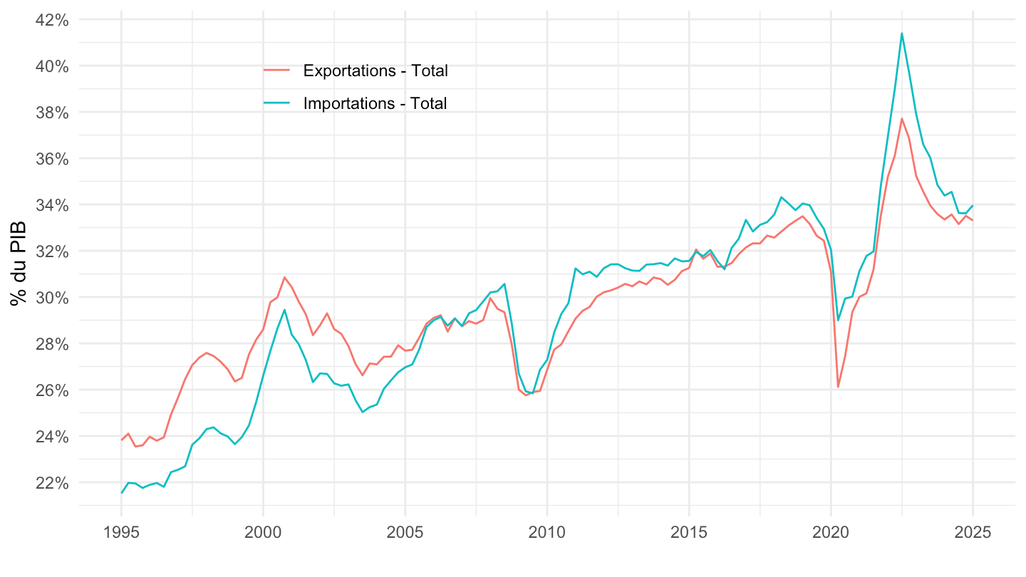
Solde Extérieur
All
Code
`CNT-2020-PIB-EQB-RF` %>%
  filter(FREQ == "T",
         VALORISATION == "V",
         OPERATION %in% c("SOLDE", "PIB")) %>%
  quarter_to_date %>%
  group_by(date) %>%
  mutate(OBS_VALUE = OBS_VALUE/OBS_VALUE[OPERATION == "PIB"]) %>%
  filter(OPERATION != "PIB") %>%
  mutate(TITLE_FR = gsub("- Valeur aux prix courants - Série CVS-CJO", "", TITLE_FR)) %>%
  na.omit %>%
  ggplot() + ylab("% du PIB") + xlab("") + theme_minimal() +
  geom_line(aes(x = date, y = OBS_VALUE, color = TITLE_FR)) +

  scale_x_date(breaks = seq(1920, 2100, 5) %>% paste0("-01-01") %>% as.Date,
               labels = date_format("%Y")) +
  theme(legend.position = c(0.3, 0.85),
        legend.title = element_blank()) +
  scale_y_continuous(breaks = 0.01*seq(-100, 300, 1),
                     labels = percent_format(accuracy = 1))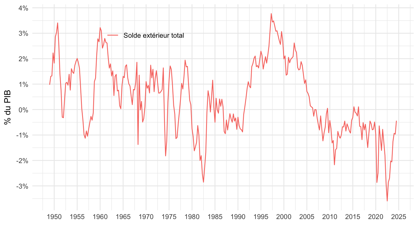
1980-
Code
`CNT-2020-PIB-EQB-RF` %>%
  filter(FREQ == "T",
         VALORISATION == "V",
         OPERATION %in% c("SOLDE", "PIB")) %>%
  quarter_to_date %>%
  group_by(date) %>%
  mutate(OBS_VALUE = OBS_VALUE/OBS_VALUE[OPERATION == "PIB"]) %>%
  filter(OPERATION != "PIB") %>%
  mutate(TITLE_FR = gsub("- Valeur aux prix courants - Série CVS-CJO", "", TITLE_FR)) %>%
  na.omit %>%
  filter(date >= as.Date("1980-01-01")) %>%
  ggplot() + ylab("% du PIB") + xlab("") + theme_minimal() +
  geom_line(aes(x = date, y = OBS_VALUE, color = TITLE_FR)) +

  scale_x_date(breaks = seq(1920, 2100, 5) %>% paste0("-01-01") %>% as.Date,
               labels = date_format("%Y")) +
  theme(legend.position = c(0.3, 0.85),
        legend.title = element_blank()) +
  scale_y_continuous(breaks = 0.01*seq(-100, 300, 1),
                     labels = percent_format(accuracy = 1))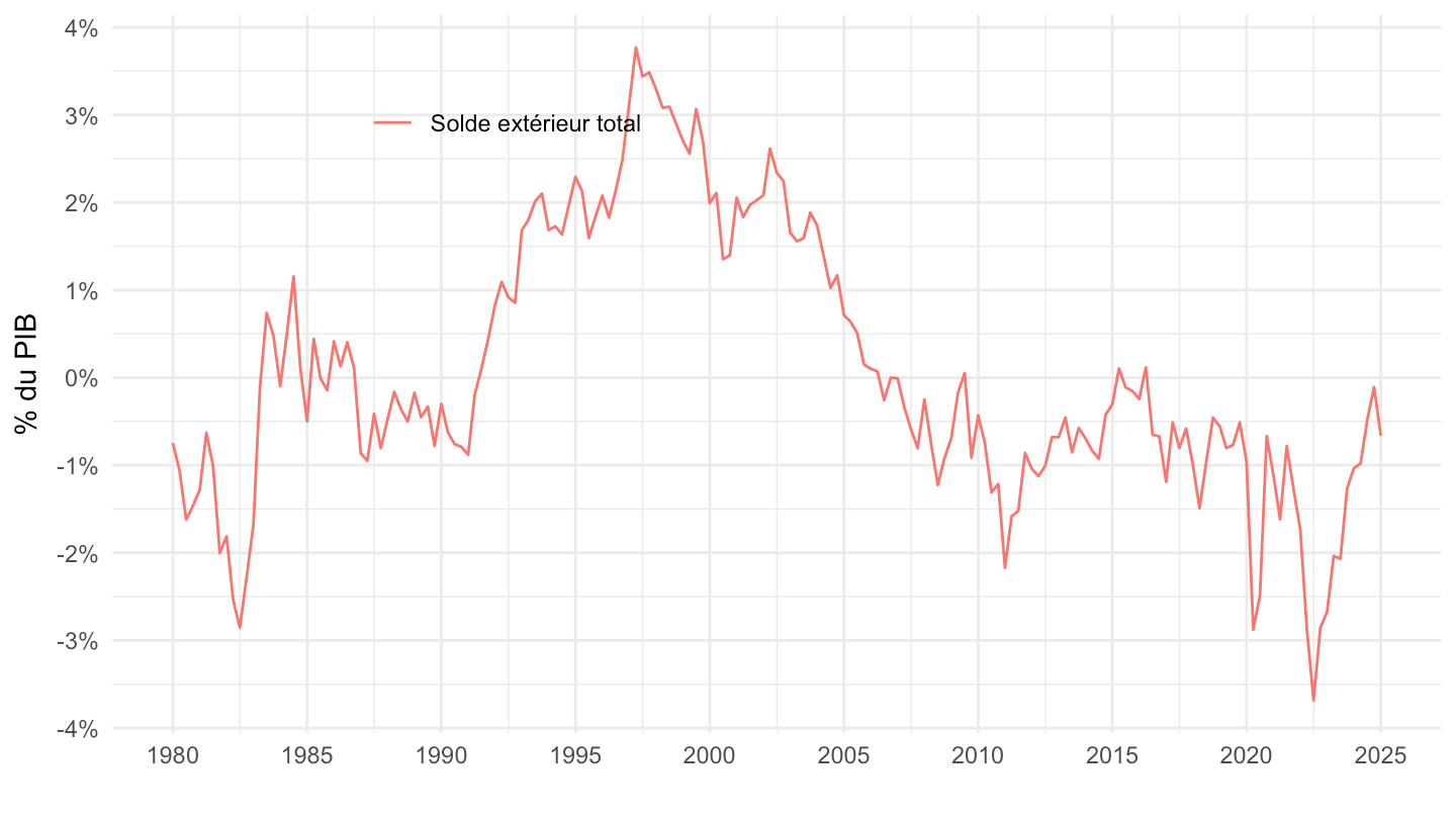
1995-
Code
`CNT-2020-PIB-EQB-RF` %>%
  filter(FREQ == "T",
         VALORISATION == "V",
         OPERATION %in% c("SOLDE", "PIB")) %>%
  quarter_to_date %>%
  group_by(date) %>%
  mutate(OBS_VALUE = OBS_VALUE/OBS_VALUE[OPERATION == "PIB"]) %>%
  filter(OPERATION != "PIB") %>%
  mutate(TITLE_FR = gsub("- Valeur aux prix courants - Série CVS-CJO", "", TITLE_FR)) %>%
  na.omit %>%
  filter(date >= as.Date("1995-01-01")) %>%
  ggplot() + ylab("% du PIB") + xlab("") + theme_minimal() +
  geom_line(aes(x = date, y = OBS_VALUE, color = TITLE_FR)) +

  scale_x_date(breaks = seq(1920, 2100, 5) %>% paste0("-01-01") %>% as.Date,
               labels = date_format("%Y")) +
  theme(legend.position = c(0.3, 0.85),
        legend.title = element_blank()) +
  scale_y_continuous(breaks = 0.01*seq(-100, 300, 1),
                     labels = percent_format(accuracy = 1))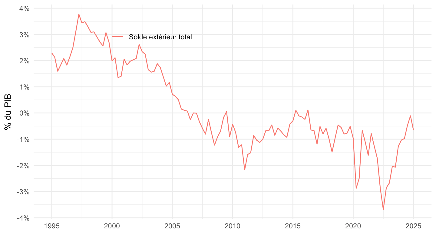
Investissement
All
Tous
Code
`CNT-2020-PIB-EQB-RF` %>%
  filter(FREQ == "T",
         VALORISATION == "V",
         OPERATION %in% c("P51", "P51B", "P51G", "P51M", "P51P", "P51S", "PIB")) %>%
  quarter_to_date %>%
  group_by(date) %>%
  mutate(OBS_VALUE = OBS_VALUE/OBS_VALUE[OPERATION == "PIB"]) %>%
  filter(OPERATION != "PIB") %>%
  mutate(TITLE_FR = gsub("- Valeur aux prix courants - Série CVS-CJO", "", TITLE_FR)) %>%
  ggplot() + ylab("% du PIB") + xlab("") + theme_minimal() +
  geom_line(aes(x = date, y = OBS_VALUE, color = paste(OPERATION, "-", TITLE_FR))) +
  #
  scale_x_date(breaks = seq(1920, 2100, 5) %>% paste0("-01-01") %>% as.Date,
               labels = date_format("%Y")) +
  theme(legend.position = c(0.3, 0.78),
        legend.title = element_blank()) +
  scale_y_continuous(breaks = 0.01*seq(0, 300, 2),
                     labels = percent_format(accuracy = 1))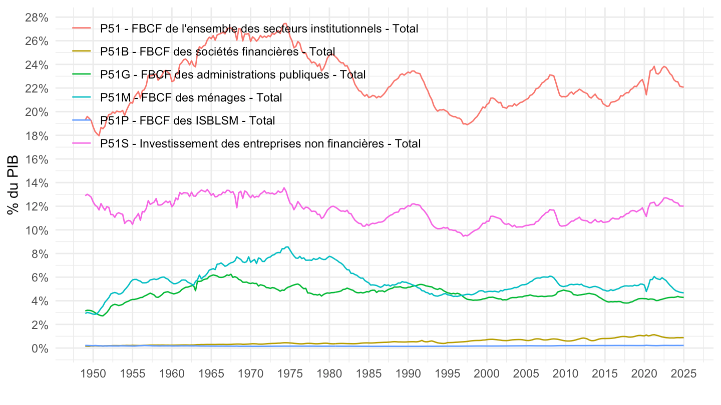
Tous sauf un
Code
`CNT-2020-PIB-EQB-RF` %>%
  filter(FREQ == "T",
         VALORISATION == "V",
         OPERATION %in% c("P51B", "P51G", "P51M", "P51P", "P51S", "PIB")) %>%
  quarter_to_date %>%
  group_by(date) %>%
  mutate(OBS_VALUE = OBS_VALUE/OBS_VALUE[OPERATION == "PIB"]) %>%
  filter(OPERATION != "PIB") %>%
  mutate(TITLE_FR = gsub("- Valeur aux prix courants - Série CVS-CJO", "", TITLE_FR)) %>%
  ggplot() + ylab("% du PIB") + xlab("") + theme_minimal() +
  geom_line(aes(x = date, y = OBS_VALUE, color = paste(OPERATION, "-", TITLE_FR))) +
  #
  scale_x_date(breaks = seq(1920, 2100, 5) %>% paste0("-01-01") %>% as.Date,
               labels = date_format("%Y")) +
  theme(legend.position = c(0.3, 0.78),
        legend.title = element_blank()) +
  scale_y_continuous(breaks = 0.01*seq(0, 300, 2),
                     labels = percent_format(accuracy = 1))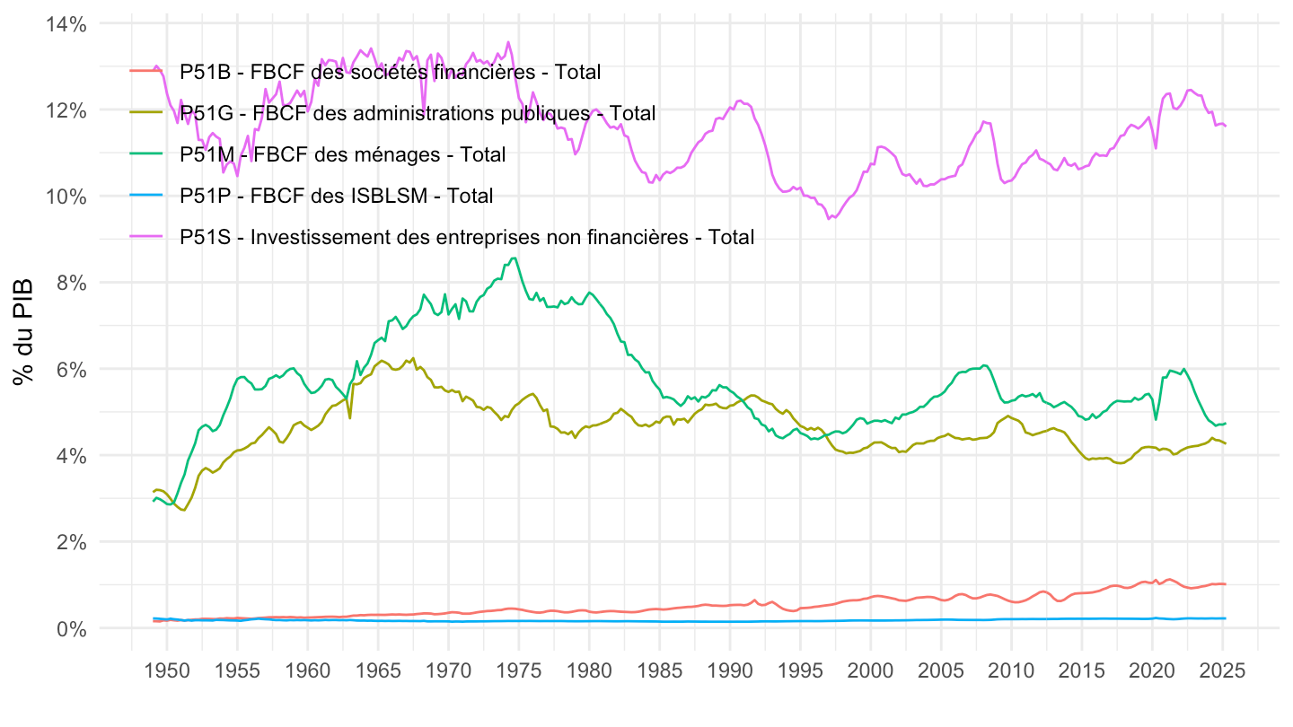
1980-
Code
`CNT-2020-PIB-EQB-RF` %>%
  filter(FREQ == "T",
         VALORISATION == "V",
         OPERATION %in% c("P51", "P51B", "P51G", "P51M", "P51P", "P51S", "PIB")) %>%
  quarter_to_date %>%
  group_by(date) %>%
  mutate(OBS_VALUE = OBS_VALUE/OBS_VALUE[OPERATION == "PIB"]) %>%
  filter(OPERATION != "PIB") %>%
  mutate(TITLE_FR = gsub("- Valeur aux prix courants - Série CVS-CJO", "", TITLE_FR)) %>%
  filter(date >= as.Date("1980-01-01")) %>%
  ggplot() + ylab("% du PIB") + xlab("") + theme_minimal() +
  geom_line(aes(x = date, y = OBS_VALUE, color = TITLE_FR)) +
  #
  scale_x_date(breaks = seq(1920, 2100, 5) %>% paste0("-01-01") %>% as.Date,
               labels = date_format("%Y")) +
  theme(legend.position = c(0.3, 0.8),
        legend.title = element_blank()) +
  scale_y_continuous(breaks = 0.01*seq(0, 300, 2),
                     labels = percent_format(accuracy = 1))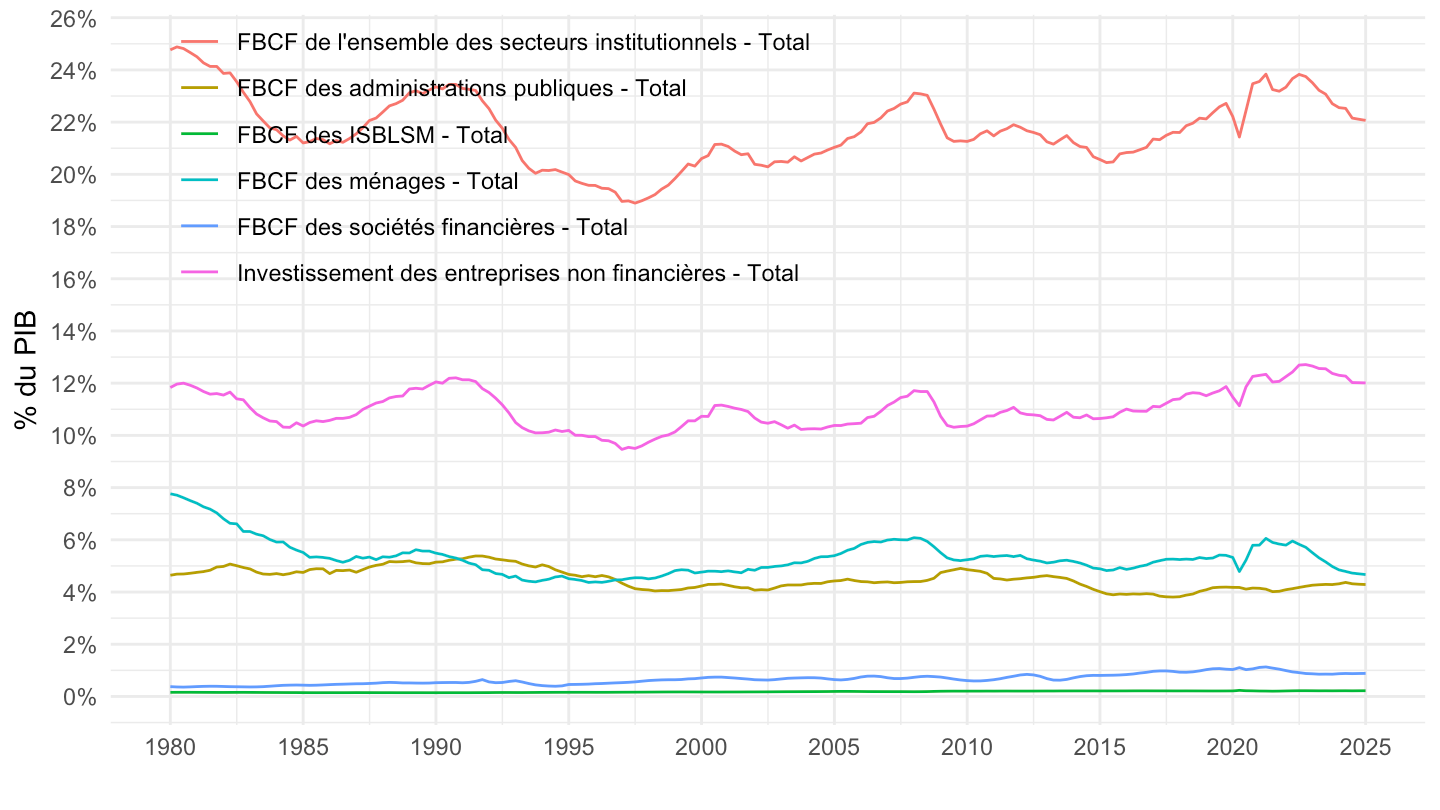
1995-
Code
`CNT-2020-PIB-EQB-RF` %>%
  filter(FREQ == "T",
         VALORISATION == "V",
         OPERATION %in% c("P51", "P51B", "P51G", "P51M", "P51P", "P51S", "PIB")) %>%
  quarter_to_date %>%
  group_by(date) %>%
  mutate(OBS_VALUE = OBS_VALUE/OBS_VALUE[OPERATION == "PIB"]) %>%
  filter(OPERATION != "PIB") %>%
  mutate(TITLE_FR = gsub("- Valeur aux prix courants - Série CVS-CJO", "", TITLE_FR)) %>%
  filter(date >= as.Date("1995-01-01")) %>%
  ggplot() + ylab("% du PIB") + xlab("") + theme_minimal() +
  geom_line(aes(x = date, y = OBS_VALUE, color = TITLE_FR)) +
  #
  scale_x_date(breaks = seq(1920, 2100, 5) %>% paste0("-01-01") %>% as.Date,
               labels = date_format("%Y")) +
  theme(legend.position = c(0.3, 0.8),
        legend.title = element_blank()) +
  scale_y_continuous(breaks = 0.01*seq(0, 300, 2),
                     labels = percent_format(accuracy = 1))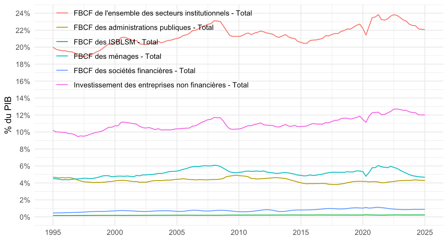
GDP Updates
gdp_quarterly2
Code
gdp_quarterly <- `CNT-2020-PIB-EQB-RF` %>%
  filter(OPERATION == "PIB",
         FREQ == "T",
         VALORISATION == "V") %>%
  quarter_to_date %>%
  arrange(date) %>%
  mutate(date = date + months(3) - days(1)) %>%
  select(date, gdp = OBS_VALUE) %>%
  mutate(gdp = gdp/1000)

save(gdp_quarterly, file = "gdp_quarterly2.RData")

gdp_quarterly %>%
  tail(5) %>%
print_table_conditional()| date | gdp |
|---|---|
| 2025-03-31 | 743.156 |
| 2025-06-30 | 745.098 |
| 2025-09-30 | 750.990 |
| 2025-12-31 | 755.888 |
| 2026-03-31 | 757.264 |
gdp_quarterly3
Code
gdp_quarterly <- `CNT-2020-PIB-EQB-RF` %>%
  filter(OPERATION == "PIB",
         FREQ == "T",
         VALORISATION == "V") %>%
  quarter_to_date %>%
  arrange(date) %>%
  select(date, gdp = OBS_VALUE) %>%
  mutate(gdp = gdp/1000)

save(gdp_quarterly, file = "gdp_quarterly3.RData")

gdp_quarterly %>%
  tail(5) %>%
print_table_conditional()| date | gdp |
|---|---|
| 2025-01-01 | 743.156 |
| 2025-04-01 | 745.098 |
| 2025-07-01 | 750.990 |
| 2025-10-01 | 755.888 |
| 2026-01-01 | 757.264 |
gdp_quarterly4: IDBANK 010565707
Code
gdp_quarterly <- `CNT-2020-PIB-EQB-RF` %>%
  filter(OPERATION == "PIB",
         FREQ == "T",
         VALORISATION == "V") %>%
  quarter_to_date %>%
  arrange(date) %>%
  select(date, gdp = OBS_VALUE)

save(gdp_quarterly, file = "gdp_quarterly4.RData")

gdp_quarterly %>%
  tail(5) %>%
print_table_conditional()| date | gdp |
|---|---|
| 2025-01-01 | 743156 |
| 2025-04-01 | 745098 |
| 2025-07-01 | 750990 |
| 2025-10-01 | 755888 |
| 2026-01-01 | 757264 |
Depuis le Covid-19
PIB valeur
Code
`CNT-2020-PIB-EQB-RF` %>%
  filter(OPERATION %in% c("PIB", "P3", "P31", "P32", "P4"),
         FREQ == "T",
         VALORISATION == "V",
         NATURE == "VALEUR_ABSOLUE",
         `SECT-INST` == "SO") %>%
  left_join(OPERATION,  by = "OPERATION") %>%
  mutate(date = zoo::as.yearqtr(TIME_PERIOD, format = "%Y-Q%q")) %>%
  filter(date >= zoo::as.yearqtr("2019 Q4")) %>%
  select_if(~ n_distinct(.) > 1) %>%
  arrange(date) %>%
  group_by(OPERATION) %>%
  mutate(OBS_VALUE = 100*OBS_VALUE/OBS_VALUE[date == zoo::as.yearqtr("2019 Q4")]) %>%
  ggplot + geom_line(aes(x = date, y = OBS_VALUE, color = Operation)) +
  xlab("") + ylab("") +  theme_minimal() +
  zoo::scale_x_yearqtr(labels = date_format("%YT%q"),
                       breaks = expand.grid(2017:2100, c(2, 4)) %>%
                         mutate(breaks = zoo::as.yearqtr(paste0(Var1, "Q", Var2))) %>%
                         pull(breaks)) +
  scale_y_log10(breaks = seq(0, 200, 5)) +
  theme(legend.position = c(0.7, 0.2),
        legend.title = element_blank(),
        axis.text.x = element_text(angle = 45, vjust = 1, hjust = 1))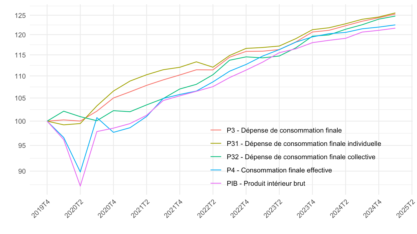
PIB volume
2019-Q4
Code
`CNT-2020-PIB-EQB-RF` %>%
  filter(OPERATION %in% c("PIB", "P3", "P31", "P32", "P4"),
         FREQ == "T",
         VALORISATION == "L",
         NATURE == "VALEUR_ABSOLUE",
         `SECT-INST` == "SO") %>%
  left_join(OPERATION,  by = "OPERATION") %>%
  mutate(date = zoo::as.yearqtr(TIME_PERIOD, format = "%Y-Q%q")) %>%
  filter(date >= zoo::as.yearqtr("2019 Q4")) %>%
  select_if(~ n_distinct(.) > 1) %>%
  arrange(date) %>%
  group_by(OPERATION) %>%
  mutate(OBS_VALUE = 100*OBS_VALUE/OBS_VALUE[date == zoo::as.yearqtr("2019 Q4")]) %>%
  ggplot + geom_line(aes(x = date, y = OBS_VALUE, color = Operation)) +
  xlab("") + ylab("") +  theme_minimal() +
  zoo::scale_x_yearqtr(labels = date_format("%YT%q"),
                       breaks = expand.grid(2017:2100, c(2, 4)) %>%
                         mutate(breaks = zoo::as.yearqtr(paste0(Var1, "Q", Var2))) %>%
                         pull(breaks)) +
  scale_y_log10(breaks = seq(0, 200, 5)) +
  theme(legend.position = c(0.7, 0.2),
        legend.title = element_blank(),
        axis.text.x = element_text(angle = 45, vjust = 1, hjust = 1))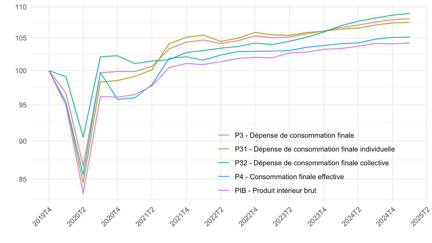
Demande, Demande hors stocks
Code
`CNT-2020-PIB-EQB-RF` %>%
  filter(OPERATION %in% c("PIB", "DINTF", "DINTFHS"),
         FREQ == "T",
         VALORISATION == "L",
         NATURE == "VALEUR_ABSOLUE",
         `SECT-INST` == "SO") %>%
  left_join(OPERATION,  by = "OPERATION") %>%
  mutate(date = zoo::as.yearqtr(TIME_PERIOD, format = "%Y-Q%q")) %>%
  filter(date >= zoo::as.yearqtr("2019 Q4")) %>%
  select_if(~ n_distinct(.) > 1) %>%
  arrange(date) %>%
  group_by(OPERATION) %>%
  mutate(OBS_VALUE = 100*OBS_VALUE/OBS_VALUE[date == zoo::as.yearqtr("2019 Q4")]) %>%
  ggplot + geom_line(aes(x = date, y = OBS_VALUE, color = Operation)) +
  xlab("") + ylab("") +  theme_minimal() +
  zoo::scale_x_yearqtr(labels = date_format("%YT%q"),
                       breaks = expand.grid(2017:2100, c(2, 4)) %>%
                         mutate(breaks = zoo::as.yearqtr(paste0(Var1, "Q", Var2))) %>%
                         pull(breaks)) +
  scale_y_log10(breaks = seq(0, 200, 5)) +
  theme(legend.position = c(0.7, 0.2),
        legend.title = element_blank(),
        axis.text.x = element_text(angle = 45, vjust = 1, hjust = 1))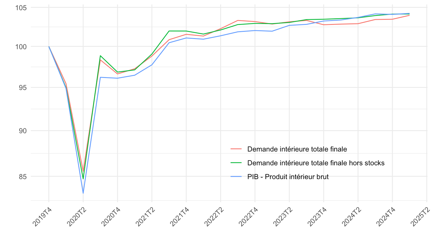
2017-Q2 -
PIB valeur
Code
`CNT-2020-PIB-EQB-RF` %>%
  filter(OPERATION %in% c("PIB", "P3", "P31", "P32", "P4"),
         FREQ == "T",
         VALORISATION == "V",
         NATURE == "VALEUR_ABSOLUE",
         `SECT-INST` == "SO") %>%
  left_join(OPERATION,  by = "OPERATION") %>%
  mutate(date = zoo::as.yearqtr(TIME_PERIOD, format = "%Y-Q%q")) %>%
  filter(date >= zoo::as.yearqtr("2017 Q2")) %>%
  select_if(~ n_distinct(.) > 1) %>%
  arrange(date) %>%
  group_by(OPERATION) %>%
  mutate(OBS_VALUE = 100*OBS_VALUE/OBS_VALUE[date == zoo::as.yearqtr("2017 Q2")]) %>%
  ggplot + geom_line(aes(x = date, y = OBS_VALUE, color = Operation)) +
  xlab("") + ylab("") +  theme_minimal() +
  zoo::scale_x_yearqtr(labels = date_format("%YT%q"),
                       breaks = expand.grid(2017:2100, c(2, 4)) %>%
                         mutate(breaks = zoo::as.yearqtr(paste0(Var1, "Q", Var2))) %>%
                         pull(breaks)) +
  scale_y_log10(breaks = seq(0, 200, 5)) +
  theme(legend.position = c(0.7, 0.2),
        legend.title = element_blank(),
        axis.text.x = element_text(angle = 45, vjust = 1, hjust = 1))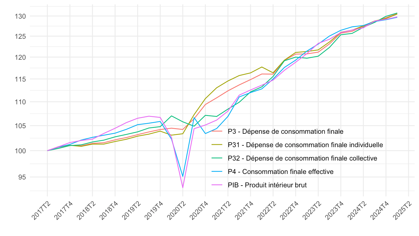
PIB volume
Code
`CNT-2020-PIB-EQB-RF` %>%
  filter(OPERATION %in% c("PIB", "P3", "P31", "P32", "P4"),
         FREQ == "T",
         VALORISATION == "L",
         NATURE == "VALEUR_ABSOLUE",
         `SECT-INST` == "SO") %>%
  left_join(OPERATION,  by = "OPERATION") %>%
  mutate(date = zoo::as.yearqtr(TIME_PERIOD, format = "%Y-Q%q")) %>%
  filter(date >= zoo::as.yearqtr("2017 Q2")) %>%
  select_if(~ n_distinct(.) > 1) %>%
  arrange(date) %>%
  group_by(OPERATION) %>%
  mutate(OBS_VALUE = 100*OBS_VALUE/OBS_VALUE[date == zoo::as.yearqtr("2017 Q2")]) %>%
  ggplot + geom_line(aes(x = date, y = OBS_VALUE, color = Operation)) +
  xlab("") + ylab("") +  theme_minimal() +
  zoo::scale_x_yearqtr(labels = date_format("%YT%q"),
                       breaks = expand.grid(2017:2100, c(2, 4)) %>%
                         mutate(breaks = zoo::as.yearqtr(paste0(Var1, "Q", Var2))) %>%
                         pull(breaks)) +
  scale_y_log10(breaks = seq(0, 200, 5)) +
  theme(legend.position = c(0.7, 0.2),
        legend.title = element_blank(),
        axis.text.x = element_text(angle = 45, vjust = 1, hjust = 1))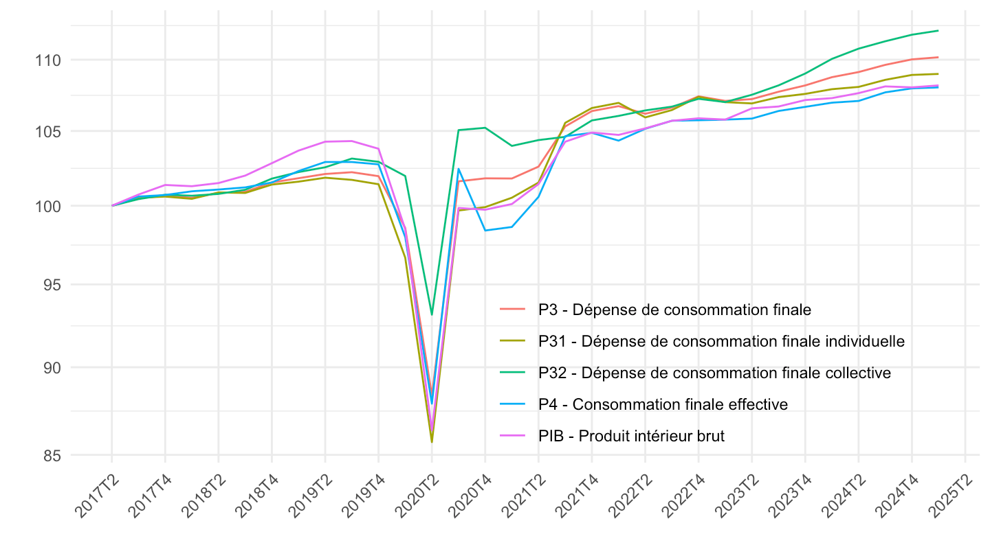
Demande, Demande hors stocks
Code
`CNT-2020-PIB-EQB-RF` %>%
  filter(OPERATION %in% c("PIB", "DINTF", "DINTFHS"),
         FREQ == "T",
         VALORISATION == "L",
         NATURE == "VALEUR_ABSOLUE",
         `SECT-INST` == "SO") %>%
  left_join(OPERATION,  by = "OPERATION") %>%
  mutate(date = zoo::as.yearqtr(TIME_PERIOD, format = "%Y-Q%q")) %>%
  filter(date >= zoo::as.yearqtr("2017 Q2")) %>%
  select_if(~ n_distinct(.) > 1) %>%
  arrange(date) %>%
  group_by(OPERATION) %>%
  mutate(OBS_VALUE = 100*OBS_VALUE/OBS_VALUE[date == zoo::as.yearqtr("2017 Q2")]) %>%
  ggplot + geom_line(aes(x = date, y = OBS_VALUE, color = Operation)) +
  xlab("") + ylab("") +  theme_minimal() +
  zoo::scale_x_yearqtr(labels = date_format("%YT%q"),
                       breaks = expand.grid(2017:2100, c(2, 4)) %>%
                         mutate(breaks = zoo::as.yearqtr(paste0(Var1, "Q", Var2))) %>%
                         pull(breaks)) +
  scale_y_log10(breaks = seq(0, 200, 2)) +
  theme(legend.position = c(0.7, 0.2),
        legend.title = element_blank(),
        axis.text.x = element_text(angle = 45, vjust = 1, hjust = 1))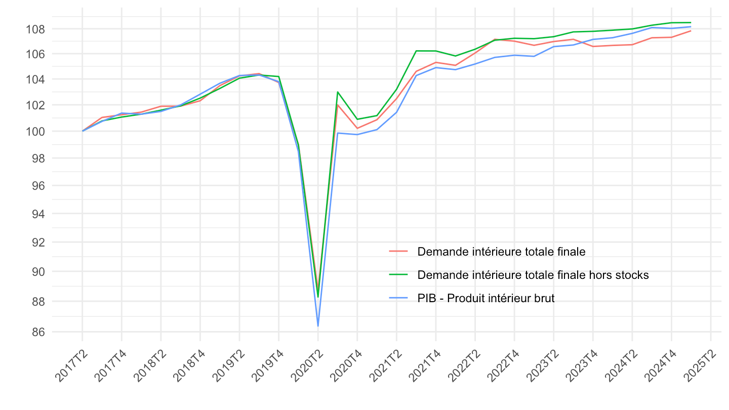
2011-Q1
PIB valeur
Code
`CNT-2020-PIB-EQB-RF` %>%
  filter(OPERATION %in% c("PIB", "P3", "P31", "P32", "P4"),
         FREQ == "T",
         VALORISATION == "V",
         NATURE == "VALEUR_ABSOLUE",
         `SECT-INST` == "SO") %>%
  left_join(OPERATION,  by = "OPERATION") %>%
  mutate(date = zoo::as.yearqtr(TIME_PERIOD, format = "%Y-Q%q")) %>%
  filter(date >= zoo::as.yearqtr("2011 Q1")) %>%
  select_if(~ n_distinct(.) > 1) %>%
  arrange(date) %>%
  group_by(OPERATION) %>%
  mutate(OBS_VALUE = 100*OBS_VALUE/OBS_VALUE[date == zoo::as.yearqtr("2011 Q1")]) %>%
  ggplot + geom_line(aes(x = date, y = OBS_VALUE, color = Operation)) +
  xlab("") + ylab("") +  theme_minimal() +
  zoo::scale_x_yearqtr(labels = date_format("%YT%q"),
                       breaks = expand.grid(2011:2100, c(2, 4)) %>%
                         mutate(breaks = zoo::as.yearqtr(paste0(Var1, "Q", Var2))) %>%
                         pull(breaks)) +
  scale_y_log10(breaks = c(seq(0, 170, 5), 106, 107, 111, 112, 113)) +
  theme(legend.position = c(0.3, 0.8),
        legend.title = element_blank(),
        axis.text.x = element_text(angle = 45, vjust = 1, hjust = 1))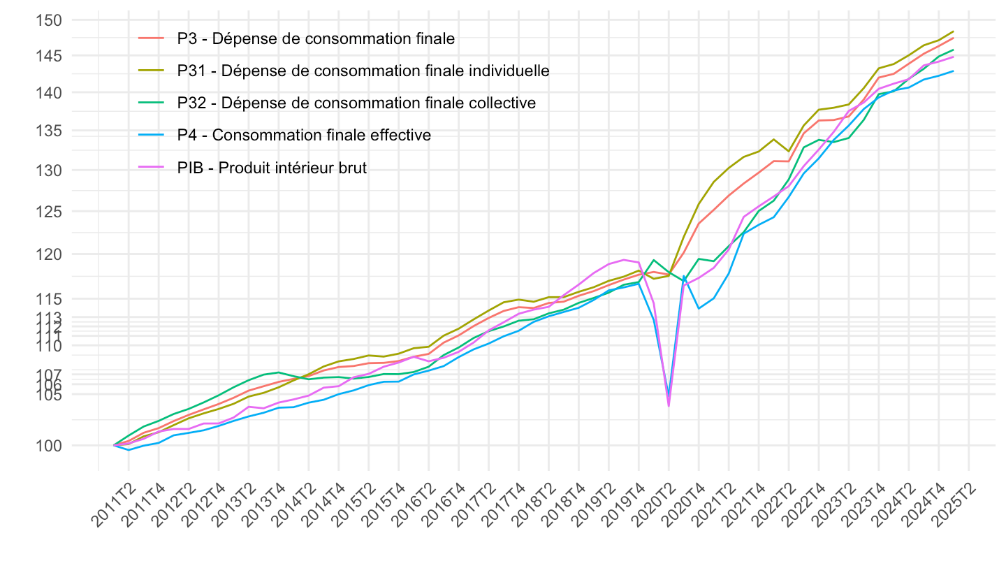
PIB volume
Code
`CNT-2020-PIB-EQB-RF` %>%
  filter(OPERATION %in% c("PIB", "P3", "P31", "P32", "P4"),
         FREQ == "T",
         VALORISATION == "L",
         NATURE == "VALEUR_ABSOLUE",
         `SECT-INST` == "SO") %>%
  left_join(OPERATION,  by = "OPERATION") %>%
  quarter_to_date %>%
  filter(date >= as.Date("2010-01-01")) %>%
  select_if(~ n_distinct(.) > 1) %>%
  arrange(date) %>%
  group_by(OPERATION) %>%
  mutate(OBS_VALUE = 100*OBS_VALUE/OBS_VALUE[date == as.Date("2010-01-01")]) %>%
  ggplot + geom_line(aes(x = date, y = OBS_VALUE, color = Operation)) +
  xlab("") + ylab("") +  theme_minimal() +
  scale_x_date(breaks = "1 year",
               labels = date_format("%Y")) +
  scale_y_log10(breaks = c(seq(0, 180, 5), 106, 107)) +
  theme(legend.position = c(0.3, 0.8),
        legend.title = element_blank())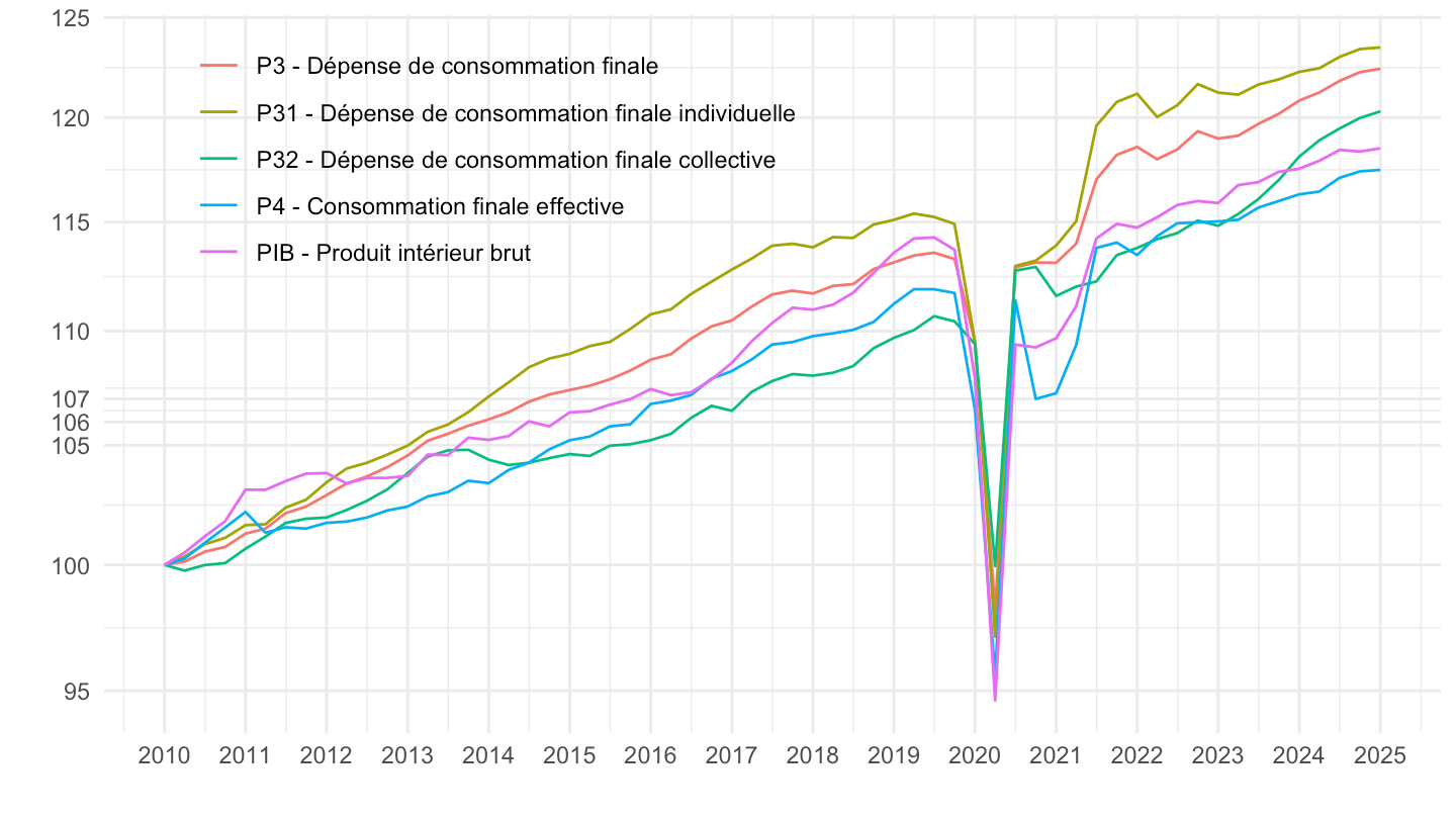
2010-2014
Code
`CNT-2020-PIB-EQB-RF` %>%
  filter(OPERATION %in% c("PIB", "P3", "P31", "P32", "P4"),
         FREQ == "T",
         VALORISATION == "L",
         NATURE == "VALEUR_ABSOLUE",
         `SECT-INST` == "SO") %>%
  left_join(OPERATION,  by = "OPERATION") %>%
  quarter_to_date %>%
  filter(date >= as.Date("2010-01-01")) %>%
  filter(date <= as.Date("2014-01-01")) %>%
  select_if(~ n_distinct(.) > 1) %>%
  arrange(date) %>%
  group_by(OPERATION) %>%
  mutate(OBS_VALUE = 100*OBS_VALUE/OBS_VALUE[date == as.Date("2010-01-01")]) %>%
  ggplot + geom_line(aes(x = date, y = OBS_VALUE, color = Operation)) +
  xlab("") + ylab("") +  theme_minimal() +
  scale_x_date(breaks = "1 year",
               labels = date_format("%Y")) +
  scale_y_log10(breaks = c(seq(100, 180, 1), 106, 107)) +
  theme(legend.position = c(0.3, 0.8),
        legend.title = element_blank())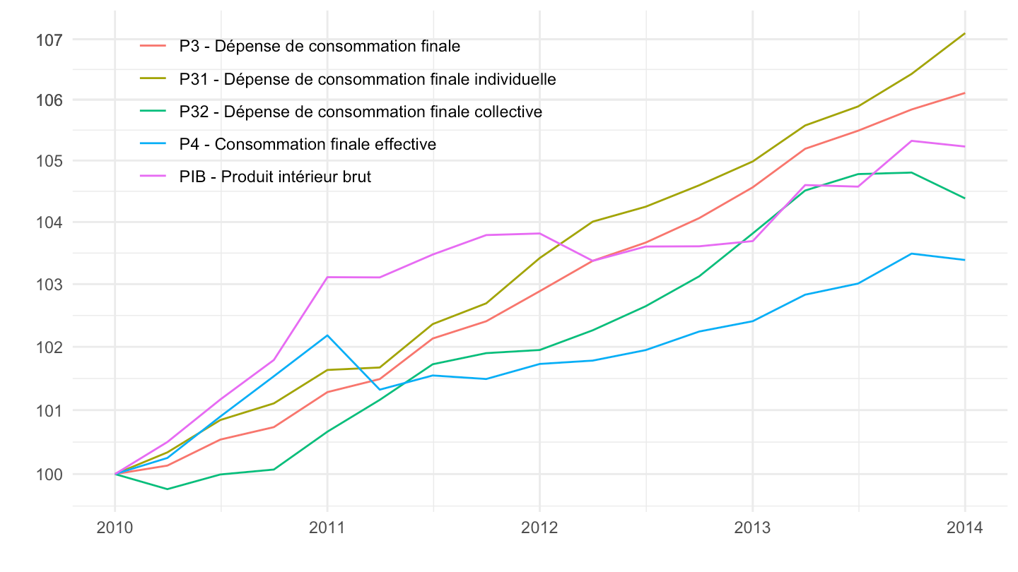
2011-2014
Code
`CNT-2020-PIB-EQB-RF` %>%
  filter(OPERATION %in% c("PIB", "P3", "P31", "P32", "P4"),
         FREQ == "T",
         VALORISATION == "L",
         NATURE == "VALEUR_ABSOLUE",
         `SECT-INST` == "SO") %>%
  left_join(OPERATION,  by = "OPERATION") %>%
  quarter_to_date %>%
  filter(date >= as.Date("2011-01-01")) %>%
  filter(date <= as.Date("2014-01-01")) %>%
  select_if(~ n_distinct(.) > 1) %>%
  arrange(date) %>%
  group_by(OPERATION) %>%
  mutate(OBS_VALUE = 100*OBS_VALUE/OBS_VALUE[date == as.Date("2011-01-01")]) %>%
  ggplot + geom_line(aes(x = date, y = OBS_VALUE, color = Operation)) +
  xlab("") + ylab("") +  theme_minimal() +
  scale_x_date(breaks = "1 year",
               labels = date_format("%Y")) +
  scale_y_log10(breaks = c(seq(100, 180, 1), 106, 107)) +
  theme(legend.position = c(0.3, 0.8),
        legend.title = element_blank())
2011-14
PIB valeur
Code
`CNT-2020-PIB-EQB-RF` %>%
  filter(OPERATION %in% c("PIB", "P3", "P31", "P32", "P4"),
         FREQ == "T",
         VALORISATION == "V",
         NATURE == "VALEUR_ABSOLUE",
         `SECT-INST` == "SO") %>%
  left_join(OPERATION,  by = "OPERATION") %>%
  quarter_to_date %>%
  filter(date >= as.Date("2011-01-01"),
         date <= as.Date("2014-01-01")) %>%
  select_if(~ n_distinct(.) > 1) %>%
  arrange(date) %>%
  group_by(OPERATION) %>%
  mutate(OBS_VALUE = 100*OBS_VALUE/OBS_VALUE[date == as.Date("2011-01-01")]) %>%
  ggplot + geom_line(aes(x = date, y = OBS_VALUE, color = Operation)) +
  xlab("") + ylab("") +  theme_minimal() +
  scale_x_date(breaks = "1 year",
               labels = date_format("%Y")) +
  scale_y_log10(breaks = c(seq(0, 170, 1), 106, 107, 111, 112, 113)) +
  theme(legend.position = c(0.3, 0.8),
        legend.title = element_blank())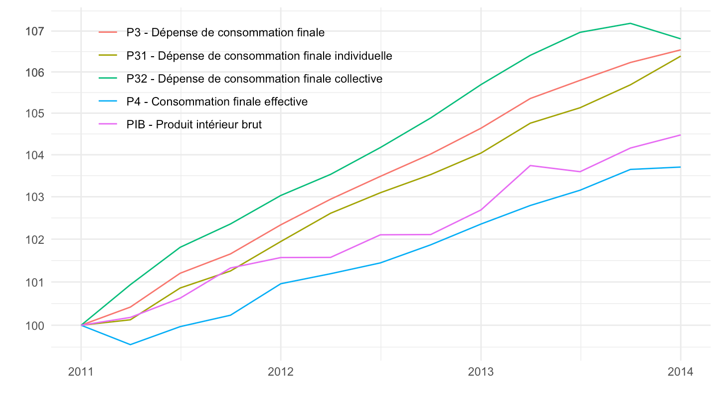
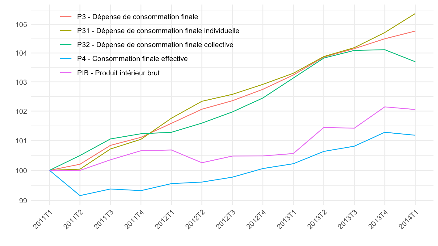
PIB volume
Code
`CNT-2020-PIB-EQB-RF` %>%
  filter(OPERATION %in% c("PIB", "P3", "P31", "P32", "P4"),
         FREQ == "T",
         VALORISATION == "L",
         NATURE == "VALEUR_ABSOLUE",
         `SECT-INST` == "SO") %>%
  left_join(OPERATION,  by = "OPERATION") %>%
  mutate(date = zoo::as.yearqtr(TIME_PERIOD, format = "%Y-Q%q")) %>%
  filter(date >= zoo::as.yearqtr("2011 Q1"),
         date <= zoo::as.yearqtr("2014 Q1")) %>%
  select_if(~ n_distinct(.) > 1) %>%
  arrange(date) %>%
  group_by(OPERATION) %>%
  mutate(OBS_VALUE = 100*OBS_VALUE/OBS_VALUE[date == zoo::as.yearqtr("2011 Q1")]) %>%
  ggplot + geom_line(aes(x = date, y = OBS_VALUE, color = Operation)) +
  xlab("") + ylab("") +  theme_minimal() +
  zoo::scale_x_yearqtr(labels = date_format("%YT%q"),
                       breaks = expand.grid(2011:2100, c(1, 2, 3, 4)) %>%
                         mutate(breaks = zoo::as.yearqtr(paste0(Var1, "Q", Var2))) %>%
                         pull(breaks)) +
  scale_y_log10(breaks = c(seq(0, 170, 1), 106, 107, 111, 112, 113)) +
  theme(legend.position = c(0.3, 0.8),
        legend.title = element_blank(),
        axis.text.x = element_text(angle = 45, vjust = 1, hjust = 1))