| source | dataset | Title | .html | .rData |
|---|---|---|---|---|
| imf | GGXCNL_G01_GDP_PT | Net lending/borrowing (also referred as overall balance) (% of GDP) | 2026-08-10 | 2026-08-01 |
| imf | GGXONLB_G01_GDP_PT | Primary net lending/borrowing (also referred as primary balance) (% of GDP) | 2026-08-10 | 2026-08-01 |
Fiscal Monitor
Data - IMF
Info
Data on public debt
| source | dataset | Title | .html | .rData |
|---|---|---|---|---|
| imf | GGXCNL_G01_GDP_PT | Net lending/borrowing (also referred as overall balance) (% of GDP) | 2026-08-10 | 2026-08-01 |
| eurostat | ei_mfir_m | Interest rates - monthly data | 2026-08-11 | 2026-08-10 |
| eurostat | gov_10q_ggdebt | Quarterly government debt | 2026-08-11 | 2026-08-10 |
| fred | r | Interest Rates | 2026-08-10 | 2026-08-10 |
| fred | saving | Saving - saving | 2026-08-10 | 2026-08-10 |
| gfd | debt | Debt | 2021-08-22 | 2026-08-01 |
| imf | FM | Fiscal Monitor (FM) | 2026-07-25 | 2026-08-10 |
| imf | GGXONLB_G01_GDP_PT | Primary net lending/borrowing (also referred as primary balance) (% of GDP) | 2026-08-10 | 2026-08-01 |
| imf | GGXWDN_G01_GDP_PT | Net debt (% of GDP) | 2026-08-10 | 2026-08-01 |
| imf | HPDD | NA | NA | NA |
| oecd | QASA_TABLE7PSD | Quarterly Sector Accounts - Public Sector Debt, consolidated, nominal value | 2026-08-11 | 2026-08-02 |
| wdi | GC.DOD.TOTL.GD.ZS | Central government debt, total (% of GDP) | 2026-08-10 | 2026-08-10 |
| wdi | GC.XPN.INTP.CN | Interest payments (current LCU) | 2026-08-10 | 2026-08-10 |
| wdi | GC.XPN.INTP.RV.ZS | Interest payments (% of revenue) | 2026-08-10 | 2026-08-10 |
| wdi | GC.XPN.INTP.ZS | Interest payments (% of expense) | 2026-08-10 | 2026-08-10 |
LAST_COMPILE
| LAST_COMPILE |
|---|
| 2026-08-11 |
Last
Code
FM |>
  group_by(date) |>
  summarise(Nobs = n()) |>
  arrange(desc(date)) |>
  head(1) |>
print_table_conditional()| date | Nobs |
|---|---|
| 2030-01-01 | 594 |
Main Datasets
Javascript
Code
INDICATOR |>
  filter(INDICATOR %in% gsub(".qmd$", "", list.files(pattern = "\\.qmd$"))) |>
  mutate(html = paste0('<a  target=_blank href=', INDICATOR, '.html > html </a>')) %>%
  {if (is_html_output()) datatable(., filter = 'top', rownames = F, escape = F) else .}
Flat
Code
INDICATOR |>
  filter(INDICATOR %in% gsub(".qmd$", "", list.files(pattern = "\\.qmd$"))) |>
  mutate(html = paste0("[html](", INDICATOR, '.html)')) %>%
{if (is_html_output()) print_table(.) else .}| INDICATOR | Indicator | html |
|---|---|---|
| GGCB_G01_PGDP_PT | Cyclically adjusted balance (% of potential GDP) | [html] |
| GGCBP_G01_PGDP_PT | Cyclically adjusted primary balance (% of potential GDP) | [html] |
| G_XWDG_G01_GDP_PT | Gross debt (% of GDP) | [html] |
| GGXWDN_G01_GDP_PT | Net debt (% of GDP) | [html] |
| GGXCNL_G01_GDP_PT | Net lending/borrowing (also referred as overall balance) (% of GDP) | [html] |
| GGXONLB_G01_GDP_PT | Primary net lending/borrowing (also referred as primary balance) (% of GDP) | [html] |
Other Datasets
Code
INDICATOR |>
  filter(!(INDICATOR %in% gsub(".qmd$", "", list.files(pattern = "\\.qmd$")))) %>%
  {if (is_html_output()) datatable(., filter = 'top', rownames = F) else .}
Interest payment
Italy, France, Germany
Code
GGXCNL_G01_GDP_PT |>
  bind_rows(GGXONLB_G01_GDP_PT) |>
  filter(REF_AREA %in% c("IT", "FR", "DE")) |>
  left_join(REF_AREA, by = "REF_AREA") |>
  year_to_date2() |>
  spread(INDICATOR, OBS_VALUE) |>
  transmute(date, Ref_area, OBS_VALUE = GGXCNL_G01_GDP_PT - GGXONLB_G01_GDP_PT) |>
  left_join(colors, by = c("Ref_area" = "country")) |>
  mutate(OBS_VALUE = OBS_VALUE/100) |>
  rename(Counterpart_area = Ref_area) |>
  #filter(date <= as.Date("2021-01-01")) %>%
  ggplot() + geom_line(aes(x = date, y = OBS_VALUE, color = color)) +
  theme_minimal() + xlab("") + ylab("Interest payments, % of GDP") +
  scale_color_identity() + add_flags +
  scale_x_date(breaks = seq(1920, 2100, 5) |> paste0("-01-01") |> as.Date(),
               labels = date_format("%Y")) +
  theme(legend.position = c(0.63, 0.9),
        legend.title = element_blank()) +
  scale_y_continuous(breaks = 0.01*seq(-60, 60, 1),
                     labels = scales::percent_format(accuracy = 1)) +
  geom_hline(yintercept = 0, linetype = "dashed", color = "black")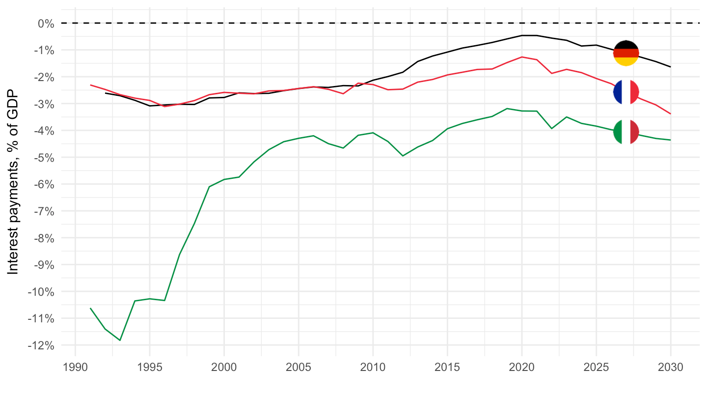
Portugal, Spain, Greece
Code
GGXCNL_G01_GDP_PT |>
  bind_rows(GGXONLB_G01_GDP_PT) |>
  filter(REF_AREA %in% c("PT", "ES", "GR")) |>
  left_join(REF_AREA, by = "REF_AREA") |>
  year_to_date2() |>
  spread(INDICATOR, OBS_VALUE) |>
  transmute(date, Ref_area, OBS_VALUE = GGXCNL_G01_GDP_PT - GGXONLB_G01_GDP_PT) |>
  left_join(colors, by = c("Ref_area" = "country")) |>
  mutate(OBS_VALUE = OBS_VALUE/100) |>
  rename(Counterpart_area = Ref_area) |>
  #filter(date <= as.Date("2021-01-01")) %>%
  ggplot() + geom_line(aes(x = date, y = OBS_VALUE, color = color)) +
  theme_minimal() + xlab("") + ylab("Interest payments, % of GDP") +
  scale_color_identity() + add_flags +
  scale_x_date(breaks = seq(1920, 2100, 5) |> paste0("-01-01") |> as.Date(),
               labels = date_format("%Y")) +
  theme(legend.position = c(0.63, 0.9),
        legend.title = element_blank()) +
  scale_y_continuous(breaks = 0.01*seq(-60, 60, 1),
                     labels = scales::percent_format(accuracy = 1)) +
  geom_hline(yintercept = 0, linetype = "dashed", color = "black")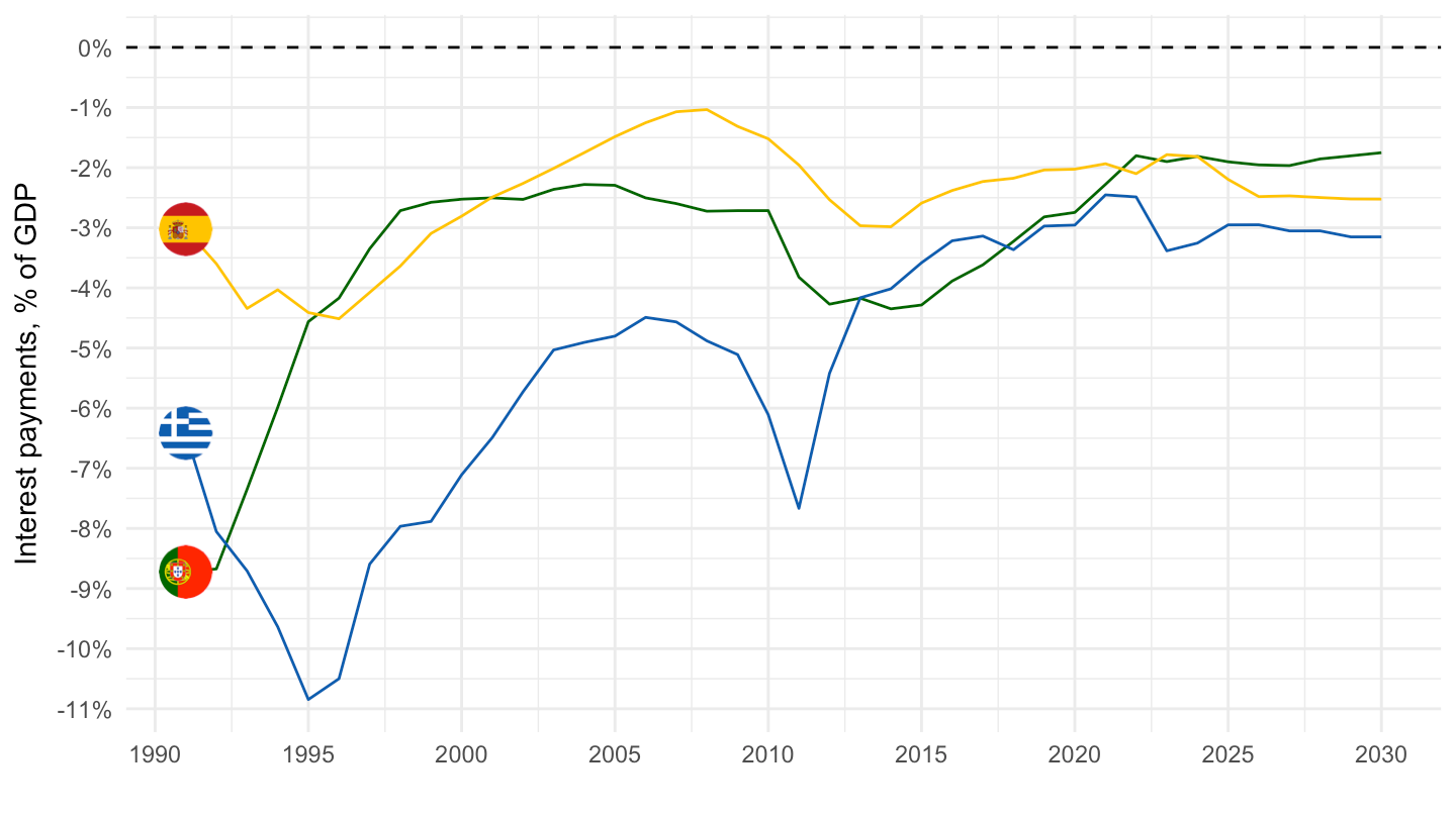
Primary / Total lending borrowing
Italy, France, Germany
Same
Code
GGXCNL_G01_GDP_PT |>
  bind_rows(GGXONLB_G01_GDP_PT) |>
  filter(REF_AREA %in% c("IT", "FR", "DE")) |>
  left_join(REF_AREA, by = "REF_AREA") |>
  year_to_date2() |>
  left_join(colors, by = c("Ref_area" = "country")) |>
  left_join(INDICATOR, by = "INDICATOR") |>
  mutate(OBS_VALUE = OBS_VALUE/100) |>
  rename(Counterpart_area = Ref_area) |>
  #filter(date <= as.Date("2021-01-01")) %>%
  ggplot() + geom_line(aes(x = date, y = OBS_VALUE, color = color, linetype = Indicator)) +
  theme_minimal() + xlab("") + ylab("Deficit, % of GDP") +
  scale_color_identity() + add_flags +
  scale_x_date(breaks = seq(1920, 2100, 5) |> paste0("-01-01") |> as.Date(),
               labels = date_format("%Y")) +
  theme(legend.position = c(0.63, 0.9),
        legend.title = element_blank()) +
  scale_y_continuous(breaks = 0.01*seq(-60, 60, 1),
                     labels = scales::percent_format(accuracy = 1)) +
  geom_hline(yintercept = 0, linetype = "dashed", color = "black")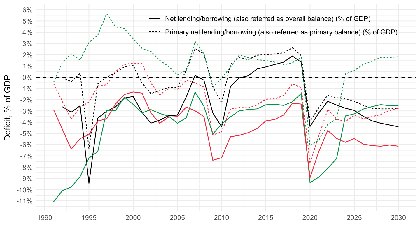
Facet Indicator
Without interest payments
Code
GGXCNL_G01_GDP_PT |>
  bind_rows(GGXONLB_G01_GDP_PT) |>
  filter(REF_AREA %in% c("IT", "FR", "DE")) |>
  left_join(REF_AREA, by = "REF_AREA") |>
  year_to_date2() |>
  left_join(colors, by = c("Ref_area" = "country")) |>
  left_join(INDICATOR, by = "INDICATOR") |>
  mutate(OBS_VALUE = OBS_VALUE/100) |>
  rename(Counterpart_area = Ref_area) |>
  mutate(Indicator = gsub("\\(also", "\n \\(also", Indicator)) |>
  ggplot() + geom_line(aes(x = date, y = OBS_VALUE, color = color)) +
  theme_minimal() + xlab("") + ylab("Deficit, % of GDP") +
  scale_color_identity() + add_flags +
  scale_x_date(breaks = seq(1920, 2100, 5) |> paste0("-01-01") |> as.Date(),
               labels = date_format("%Y")) +
  theme(legend.position = c(0.63, 0.9),
        legend.title = element_blank()) +
  scale_y_continuous(breaks = 0.01*seq(-60, 60, 1),
                     labels = scales::percent_format(accuracy = 1)) +
  geom_hline(yintercept = 0, linetype = "dashed", color = "black") +
  facet_wrap(~ Indicator)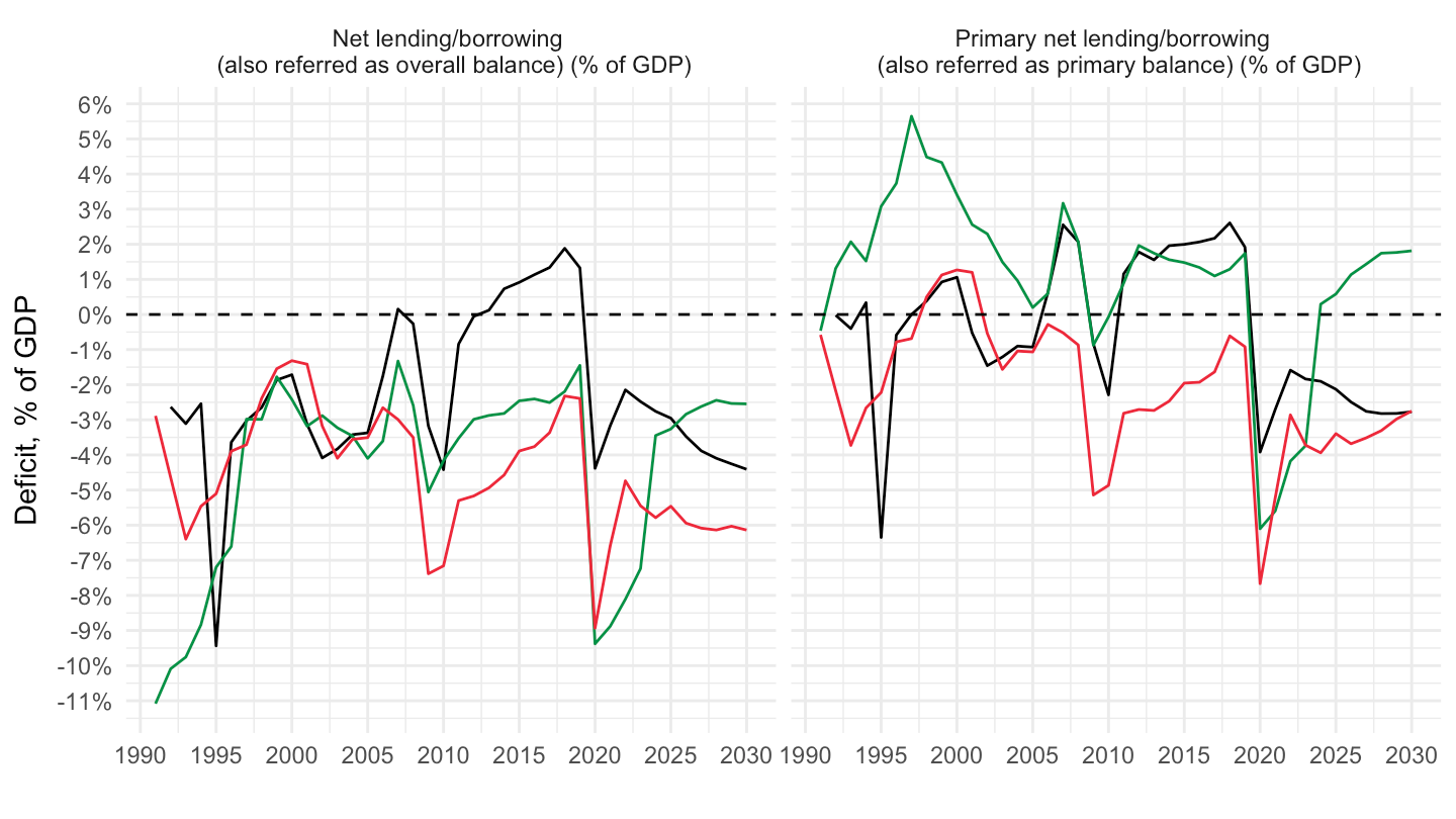
With interest payments
Code
GGXCNL_G01_GDP_PT |>
  bind_rows(GGXONLB_G01_GDP_PT) |>
  filter(REF_AREA %in% c("IT", "FR", "DE")) |>
  left_join(REF_AREA, by = "REF_AREA") |>
  year_to_date2() |>
  left_join(colors, by = c("Ref_area" = "country")) |>
  spread(INDICATOR, OBS_VALUE) |>
  mutate(GGXCIP_G01_GDP_PT = GGXCNL_G01_GDP_PT - GGXONLB_G01_GDP_PT) |>
  gather(INDICATOR, OBS_VALUE, GGXCIP_G01_GDP_PT, GGXCIP_G01_GDP_PT, GGXCNL_G01_GDP_PT, GGXONLB_G01_GDP_PT) |>
  left_join(tribble(~ INDICATOR, ~ Indicator,
                    "GGXCIP_G01_GDP_PT", "Interest payments (% of GDP)",
                    "GGXCNL_G01_GDP_PT", "Overall balance (% of GDP)",
                    "GGXONLB_G01_GDP_PT", "Primary balance (% of GDP)"), by = "INDICATOR") |>
  mutate(Indicator = factor(Indicator, levels = c("Overall balance (% of GDP)", "Interest payments (% of GDP)", "Primary balance (% of GDP)"))) |>
  mutate(OBS_VALUE = OBS_VALUE/100) |>
  rename(Counterpart_area = Ref_area) |>
  ggplot() + geom_line(aes(x = date, y = OBS_VALUE, color = color)) +
  theme_minimal() + xlab("") + ylab("% of GDP") +
  scale_color_identity() + add_flags +
  scale_x_date(breaks = seq(1920, 2100, 5) |> paste0("-01-01") |> as.Date(),
               labels = date_format("%Y")) +
  theme(legend.position = c(0.63, 0.9),
        legend.title = element_blank(),
        axis.text.x = element_text(angle = 45, vjust = 1, hjust = 1)) +
  scale_y_continuous(breaks = 0.01*seq(-60, 60, 1),
                     labels = scales::percent_format(accuracy = 1)) +
  geom_hline(yintercept = 0, linetype = "dashed", color = "black") +
  facet_wrap(~ Indicator)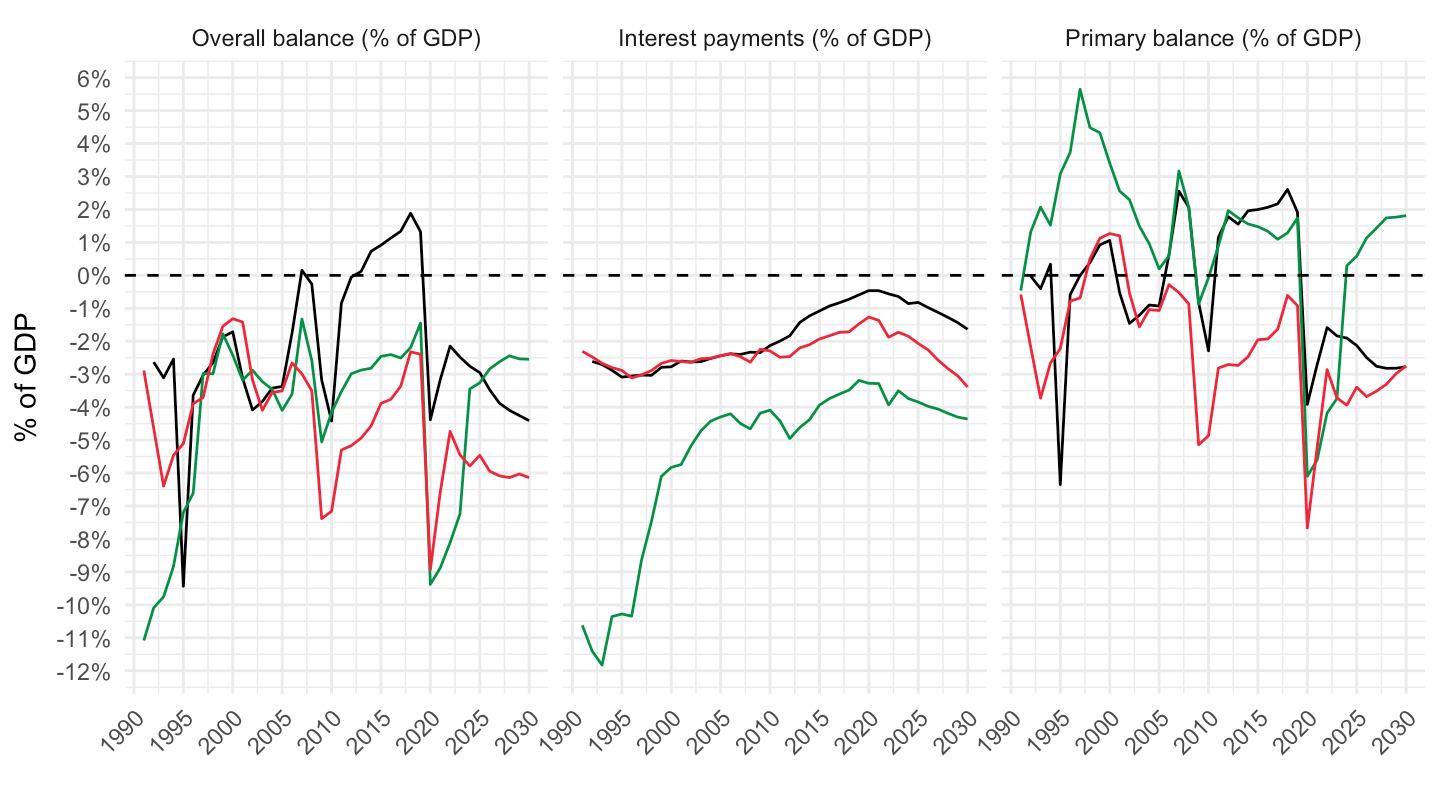
Facet country
Without interest payments
Code
GGXCNL_G01_GDP_PT |>
  bind_rows(GGXONLB_G01_GDP_PT) |>
  filter(REF_AREA %in% c("IT", "FR", "DE")) |>
  left_join(REF_AREA, by = "REF_AREA") |>
  year_to_date2() |>
  left_join(INDICATOR, by = "INDICATOR") |>
  mutate(OBS_VALUE = OBS_VALUE/100) |>
  ggplot() + geom_line(aes(x = date, y = OBS_VALUE, color = Indicator)) +
  theme_minimal() + xlab("") + ylab("Deficit, % of GDP") +
  scale_x_date(breaks = seq(1920, 2100, 5) |> paste0("-01-01") |> as.Date(),
               labels = date_format("%Y")) +
  theme(legend.position = c(0.35, 0.9),
        legend.title = element_blank(),
        axis.text.x = element_text(angle = 45, vjust = 1, hjust = 1)) +
  scale_y_continuous(breaks = 0.01*seq(-60, 60, 1),
                     labels = scales::percent_format(accuracy = 1)) +
  geom_hline(yintercept = 0, linetype = "dashed", color = "black") +
  facet_wrap(~ Ref_area)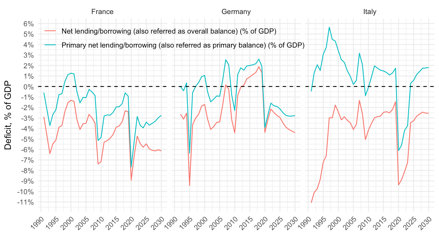
With interest payments
Code
GGXCNL_G01_GDP_PT |>
  bind_rows(GGXONLB_G01_GDP_PT) |>
  filter(REF_AREA %in% c("IT", "FR", "DE")) |>
  left_join(REF_AREA, by = "REF_AREA") |>
  year_to_date2() |>
  spread(INDICATOR, OBS_VALUE) |>
  mutate(GGXCIP_G01_GDP_PT = GGXCNL_G01_GDP_PT - GGXONLB_G01_GDP_PT) |>
  gather(INDICATOR, OBS_VALUE, GGXCIP_G01_GDP_PT, GGXCIP_G01_GDP_PT, GGXCNL_G01_GDP_PT, GGXONLB_G01_GDP_PT) |>
  left_join(tribble(~ INDICATOR, ~ Indicator,
                    "GGXCIP_G01_GDP_PT", "Interest payments (% of GDP)",
                    "GGXCNL_G01_GDP_PT", "Overall balance (% of GDP)",
                    "GGXONLB_G01_GDP_PT", "Primary balance (% of GDP)"), by = "INDICATOR") |>
  mutate(Indicator = factor(Indicator, levels = c("Overall balance (% of GDP)", "Interest payments (% of GDP)", "Primary balance (% of GDP)"))) |>
  mutate(OBS_VALUE = OBS_VALUE/100) |>
  ggplot() + geom_line(aes(x = date, y = OBS_VALUE, color = Indicator)) +
  theme_minimal() + xlab("") + ylab("Deficit, % of GDP") +
  scale_x_date(breaks = seq(1920, 2100, 5) |> paste0("-01-01") |> as.Date(),
               labels = date_format("%Y")) +
  theme(legend.position = c(0.35, 0.9),
        legend.title = element_blank(),
        axis.text.x = element_text(angle = 45, vjust = 1, hjust = 1)) +
  scale_y_continuous(breaks = 0.01*seq(-60, 60, 1),
                     labels = scales::percent_format(accuracy = 1)) +
  geom_hline(yintercept = 0, linetype = "dashed", color = "black") +
  facet_wrap(~ Ref_area)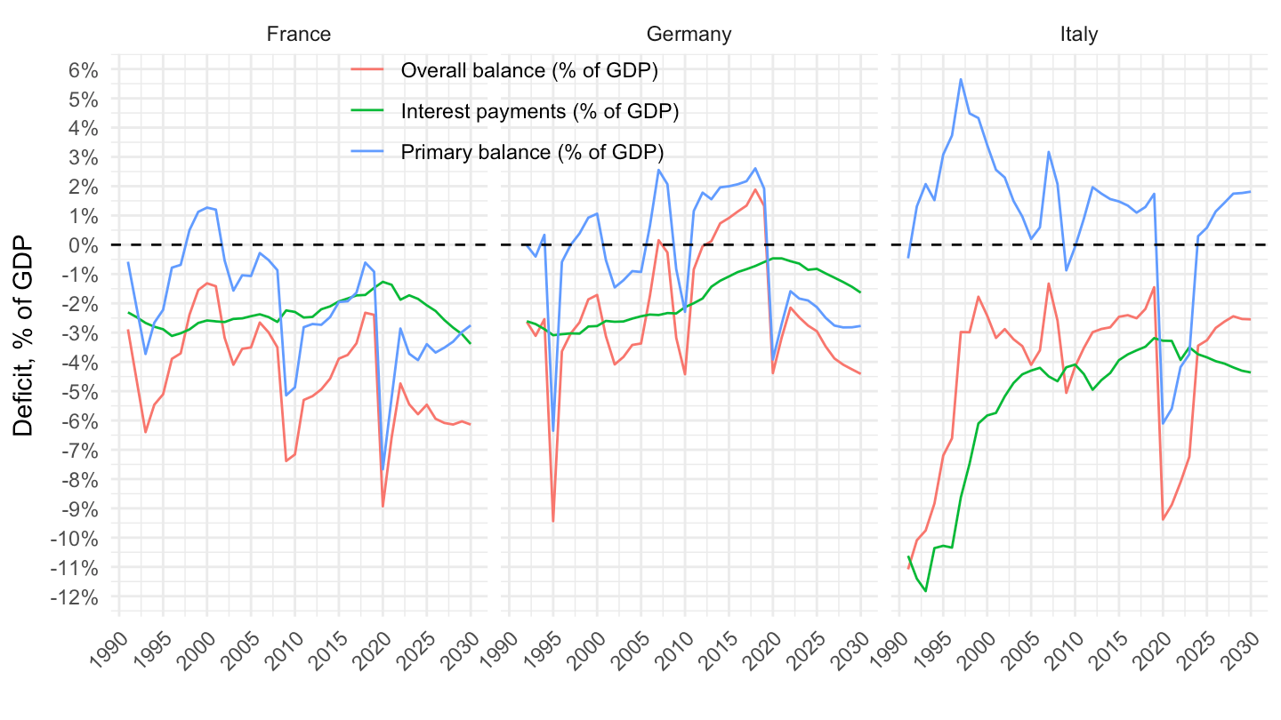
Interest Payments, Primary / Total lending
9 Biggest
Original
All
Code
GGXCNL_G01_GDP_PT |>
  bind_rows(GGXONLB_G01_GDP_PT) |>
  filter(REF_AREA %in% c("DE","FR","IT",  "ES", "NL", "BE", "AT", "PT", "FI")) |>
  left_join(REF_AREA, by = "REF_AREA") |>
  year_to_date2() |>
  spread(INDICATOR, OBS_VALUE) |>
  mutate(GGXCIP_G01_GDP_PT = GGXCNL_G01_GDP_PT - GGXONLB_G01_GDP_PT) |>
  gather(INDICATOR, OBS_VALUE, GGXCIP_G01_GDP_PT, GGXCIP_G01_GDP_PT, GGXCNL_G01_GDP_PT, GGXONLB_G01_GDP_PT) |>
  left_join(tribble(~ INDICATOR, ~ Indicator,
                    "GGXCIP_G01_GDP_PT", "Interest payments (% of GDP)",
                    "GGXCNL_G01_GDP_PT", "Overall balance (% of GDP)",
                    "GGXONLB_G01_GDP_PT", "Primary balance (% of GDP)"), by = "INDICATOR") |>
  mutate(Indicator = factor(Indicator, levels = c("Overall balance (% of GDP)", "Interest payments (% of GDP)", "Primary balance (% of GDP)"))) |>
  mutate(OBS_VALUE = OBS_VALUE/100) |>
  ggplot() + geom_line(aes(x = date, y = OBS_VALUE, color = Indicator)) +
  theme_minimal() + xlab("") + ylab("Deficit, % of GDP") +
  scale_x_date(breaks = seq(1920, 2100, 5) |> paste0("-01-01") |> as.Date(),
               labels = date_format("%Y")) +
  theme(legend.position = "top",
        legend.title = element_blank(),
        axis.text.x = element_text(angle = 45, vjust = 1, hjust = 1)) +
  scale_y_continuous(breaks = 0.01*seq(-60, 60, 5),
                     labels = scales::percent_format(accuracy = 1)) +
  geom_hline(yintercept = 0, linetype = "dashed", color = "black") +
  facet_wrap(~ Ref_area)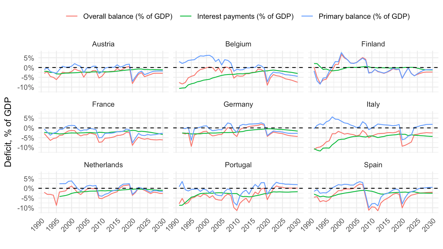
2005-2015
Code
GGXCNL_G01_GDP_PT |>
  bind_rows(GGXONLB_G01_GDP_PT) |>
  filter(REF_AREA %in% c("DE","FR","IT",  "ES", "NL", "BE", "AT", "PT", "FI")) |>
  left_join(REF_AREA, by = "REF_AREA") |>
  year_to_date2() |>
  filter(date >= as.Date("2007-01-01"),
         date <= as.Date("2014-01-01")) |>
  spread(INDICATOR, OBS_VALUE) |>
  mutate(GGXCIP_G01_GDP_PT = GGXCNL_G01_GDP_PT - GGXONLB_G01_GDP_PT) |>
  gather(INDICATOR, OBS_VALUE, GGXCIP_G01_GDP_PT, GGXCIP_G01_GDP_PT, GGXCNL_G01_GDP_PT, GGXONLB_G01_GDP_PT) |>
  left_join(tribble(~ INDICATOR, ~ Indicator,
                    "GGXCIP_G01_GDP_PT", "Interest payments (% of GDP)",
                    "GGXCNL_G01_GDP_PT", "Overall balance (% of GDP)",
                    "GGXONLB_G01_GDP_PT", "Primary balance (% of GDP)"), by = "INDICATOR") |>
  mutate(Indicator = factor(Indicator, levels = c("Overall balance (% of GDP)", "Interest payments (% of GDP)", "Primary balance (% of GDP)"))) |>
  mutate(OBS_VALUE = OBS_VALUE/100) |>
  ggplot() + geom_line(aes(x = date, y = OBS_VALUE, color = Indicator)) +
  theme_minimal() + xlab("") + ylab("Deficit, % of GDP") +
  scale_x_date(breaks = seq(1920, 2100, 1) |> paste0("-01-01") |> as.Date(),
               labels = date_format("%Y")) +
  theme(legend.position = "top",
        legend.title = element_blank(),
        axis.text.x = element_text(angle = 45, vjust = 1, hjust = 1)) +
  scale_y_continuous(breaks = 0.01*seq(-60, 60, 5),
                     labels = scales::percent_format(accuracy = 1)) +
  geom_hline(yintercept = 0, linetype = "dashed", color = "black") +
  facet_wrap(~ Ref_area)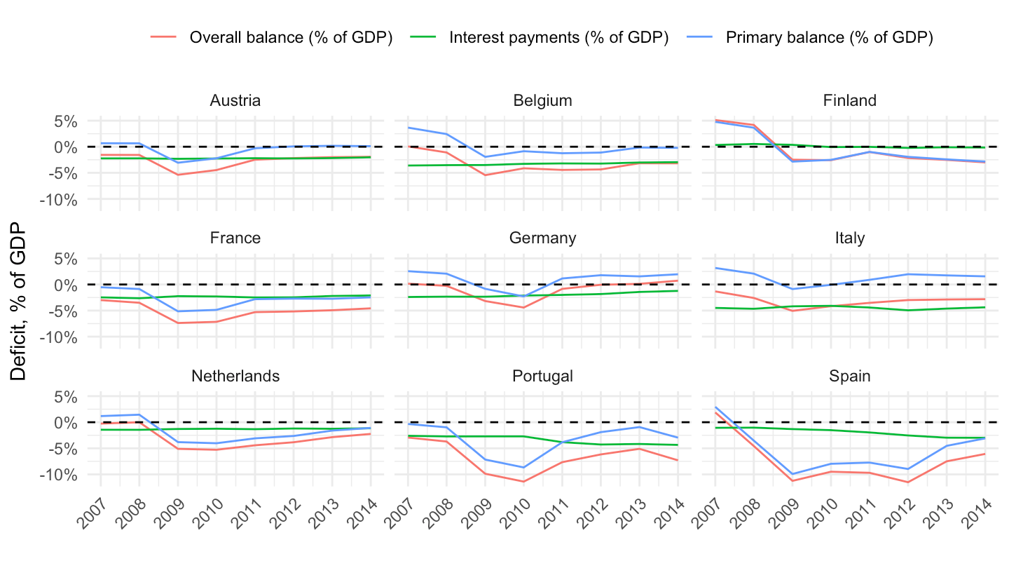
Only interest payments
Code
GGXCNL_G01_GDP_PT |>
  bind_rows(GGXONLB_G01_GDP_PT) |>
  filter(REF_AREA %in% c("DE","FR","IT",  "ES", "NL", "BE", "AT", "PT", "FI")) |>
  left_join(REF_AREA, by = "REF_AREA") |>
  year_to_date2() |>
  filter(date >= as.Date("2007-01-01"),
         date <= as.Date("2014-01-01")) |>
  spread(INDICATOR, OBS_VALUE) |>
  mutate(GGXCIP_G01_GDP_PT = GGXCNL_G01_GDP_PT - GGXONLB_G01_GDP_PT) |>
  select(-GGXCNL_G01_GDP_PT, -GGXONLB_G01_GDP_PT) |>
  gather(INDICATOR, OBS_VALUE, GGXCIP_G01_GDP_PT) |>
  left_join(tribble(~ INDICATOR, ~ Indicator,
                    "GGXCIP_G01_GDP_PT", "Interest payments (% of GDP)",
                    "GGXCNL_G01_GDP_PT", "Overall balance (% of GDP)",
                    "GGXONLB_G01_GDP_PT", "Primary balance (% of GDP)"), by = "INDICATOR") |>
  mutate(Indicator = factor(Indicator, levels = c("Overall balance (% of GDP)", "Interest payments (% of GDP)", "Primary balance (% of GDP)"))) |>
  mutate(OBS_VALUE = OBS_VALUE/100) |>
  ggplot() + geom_line(aes(x = date, y = OBS_VALUE, color = Indicator)) +
  theme_minimal() + xlab("") + ylab("Deficit, % of GDP") +
  scale_x_date(breaks = seq(1920, 2100, 1) |> paste0("-01-01") |> as.Date(),
               labels = date_format("%Y")) +
  theme(legend.position = "top",
        legend.title = element_blank(),
        axis.text.x = element_text(angle = 45, vjust = 1, hjust = 1)) +
  scale_y_continuous(breaks = 0.01*seq(-60, 60, 5),
                     labels = scales::percent_format(accuracy = 1)) +
  geom_hline(yintercept = 0, linetype = "dashed", color = "black") +
  facet_wrap(~ Ref_area)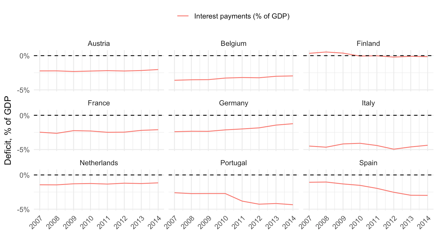
Cyclically Adjusted
Code
GGCBP_G01_PGDP_PT |>
  bind_rows(GGCB_G01_PGDP_PT) |>
  filter(REF_AREA %in% c("DE","FR","IT",  "ES", "NL", "BE", "AT", "PT", "FI")) |>
  left_join(REF_AREA, by = "REF_AREA") |>
  year_to_date2() |>
  spread(INDICATOR, OBS_VALUE) |>
  mutate(GGCBIP_G01_PGDP_PT = GGCB_G01_PGDP_PT - GGCBP_G01_PGDP_PT) |>
  gather(INDICATOR, OBS_VALUE, GGCBIP_G01_PGDP_PT, GGCB_G01_PGDP_PT, GGCBP_G01_PGDP_PT) |>
  left_join(tribble(~ INDICATOR, ~ Indicator,
                    "GGCBIP_G01_PGDP_PT", "Interest payments (% of CA GDP)",
                    "GGCB_G01_PGDP_PT", "CA Overall balance (% of CA GDP)",
                    "GGCBP_G01_PGDP_PT", "CA Primary balance (% of CA GDP)"), by = "INDICATOR") |>
  mutate(Indicator = factor(Indicator, levels = c("CA Overall balance (% of CA GDP)", "Interest payments (% of CA GDP)", "CA Primary balance (% of CA GDP)"))) |>
  mutate(OBS_VALUE = OBS_VALUE/100) |>
  ggplot() + geom_line(aes(x = date, y = OBS_VALUE, color = Indicator)) +
  theme_minimal() + xlab("") + ylab("Deficit, % of GDP") +
  scale_x_date(breaks = seq(1920, 2100, 5) |> paste0("-01-01") |> as.Date(),
               labels = date_format("%Y")) +
  theme(legend.position = "top",
        legend.title = element_blank(),
        axis.text.x = element_text(angle = 45, vjust = 1, hjust = 1)) +
  scale_y_continuous(breaks = 0.01*seq(-60, 60, 5),
                     labels = scales::percent_format(accuracy = 1)) +
  geom_hline(yintercept = 0, linetype = "dashed", color = "black") +
  facet_wrap(~ Ref_area)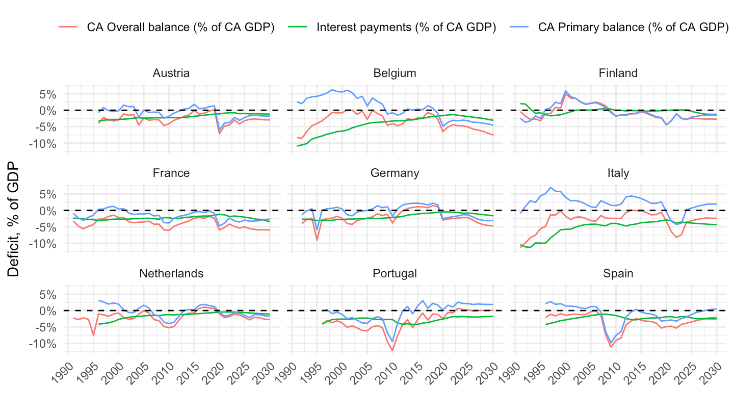
9 smallest
Code
GGXCNL_G01_GDP_PT |>
  bind_rows(GGXONLB_G01_GDP_PT) |>
  filter(REF_AREA %in% c("SK","LT",  "SI", "LU", "LV", "EE", "CY", "MT")) |>
  left_join(REF_AREA, by = "REF_AREA") |>
  year_to_date2() |>
  spread(INDICATOR, OBS_VALUE) |>
  mutate(GGXCIP_G01_GDP_PT = GGXCNL_G01_GDP_PT - GGXONLB_G01_GDP_PT) |>
  gather(INDICATOR, OBS_VALUE, GGXCIP_G01_GDP_PT, GGXCIP_G01_GDP_PT, GGXCNL_G01_GDP_PT, GGXONLB_G01_GDP_PT) |>
  left_join(tribble(~ INDICATOR, ~ Indicator,
                    "GGXCIP_G01_GDP_PT", "Interest payments (% of GDP)",
                    "GGXCNL_G01_GDP_PT", "Overall balance (% of GDP)",
                    "GGXONLB_G01_GDP_PT", "Primary balance (% of GDP)"), by = "INDICATOR") |>
  mutate(Indicator = factor(Indicator, levels = c("Overall balance (% of GDP)", "Interest payments (% of GDP)", "Primary balance (% of GDP)"))) |>
  mutate(OBS_VALUE = OBS_VALUE/100) |>
  ggplot() + geom_line(aes(x = date, y = OBS_VALUE, color = Indicator)) +
  theme_minimal() + xlab("") + ylab("Deficit, % of GDP") +
  scale_x_date(breaks = seq(1920, 2100, 5) |> paste0("-01-01") |> as.Date(),
               labels = date_format("%Y")) +
  theme(legend.position = "top",
        legend.title = element_blank(),
        axis.text.x = element_text(angle = 45, vjust = 1, hjust = 1)) +
  scale_y_continuous(breaks = 0.01*seq(-60, 60, 5),
                     labels = scales::percent_format(accuracy = 1)) +
  geom_hline(yintercept = 0, linetype = "dashed", color = "black") +
  facet_wrap(~ Ref_area)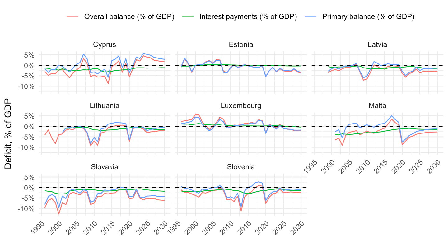
Large deficits: Ireland, Greece
Code
GGXCNL_G01_GDP_PT |>
  bind_rows(GGXONLB_G01_GDP_PT) |>
  filter(REF_AREA %in% c("IE","GR")) |>
  left_join(REF_AREA, by = "REF_AREA") |>
  year_to_date2() |>
  spread(INDICATOR, OBS_VALUE) |>
  mutate(GGXCIP_G01_GDP_PT = GGXCNL_G01_GDP_PT - GGXONLB_G01_GDP_PT) |>
  gather(INDICATOR, OBS_VALUE, GGXCIP_G01_GDP_PT, GGXCIP_G01_GDP_PT, GGXCNL_G01_GDP_PT, GGXONLB_G01_GDP_PT) |>
  left_join(tribble(~ INDICATOR, ~ Indicator,
                    "GGXCIP_G01_GDP_PT", "Interest payments (% of GDP)",
                    "GGXCNL_G01_GDP_PT", "Overall balance (% of GDP)",
                    "GGXONLB_G01_GDP_PT", "Primary balance (% of GDP)"), by = "INDICATOR") |>
  mutate(Indicator = factor(Indicator, levels = c("Overall balance (% of GDP)", "Interest payments (% of GDP)", "Primary balance (% of GDP)"))) |>
  mutate(OBS_VALUE = OBS_VALUE/100) |>
  ggplot() + geom_line(aes(x = date, y = OBS_VALUE, color = Indicator)) +
  theme_minimal() + xlab("") + ylab("Deficit, % of GDP") +
  scale_x_date(breaks = seq(1920, 2100, 5) |> paste0("-01-01") |> as.Date(),
               labels = date_format("%Y")) +
  theme(legend.position = "top",
        legend.title = element_blank(),
        axis.text.x = element_text(angle = 45, vjust = 1, hjust = 1)) +
  scale_y_continuous(breaks = 0.01*seq(-60, 60, 5),
                     labels = scales::percent_format(accuracy = 1)) +
  geom_hline(yintercept = 0, linetype = "dashed", color = "black") +
  facet_wrap(~ Ref_area)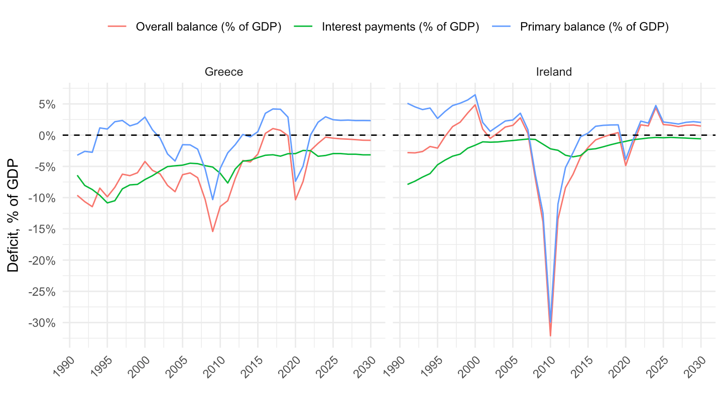
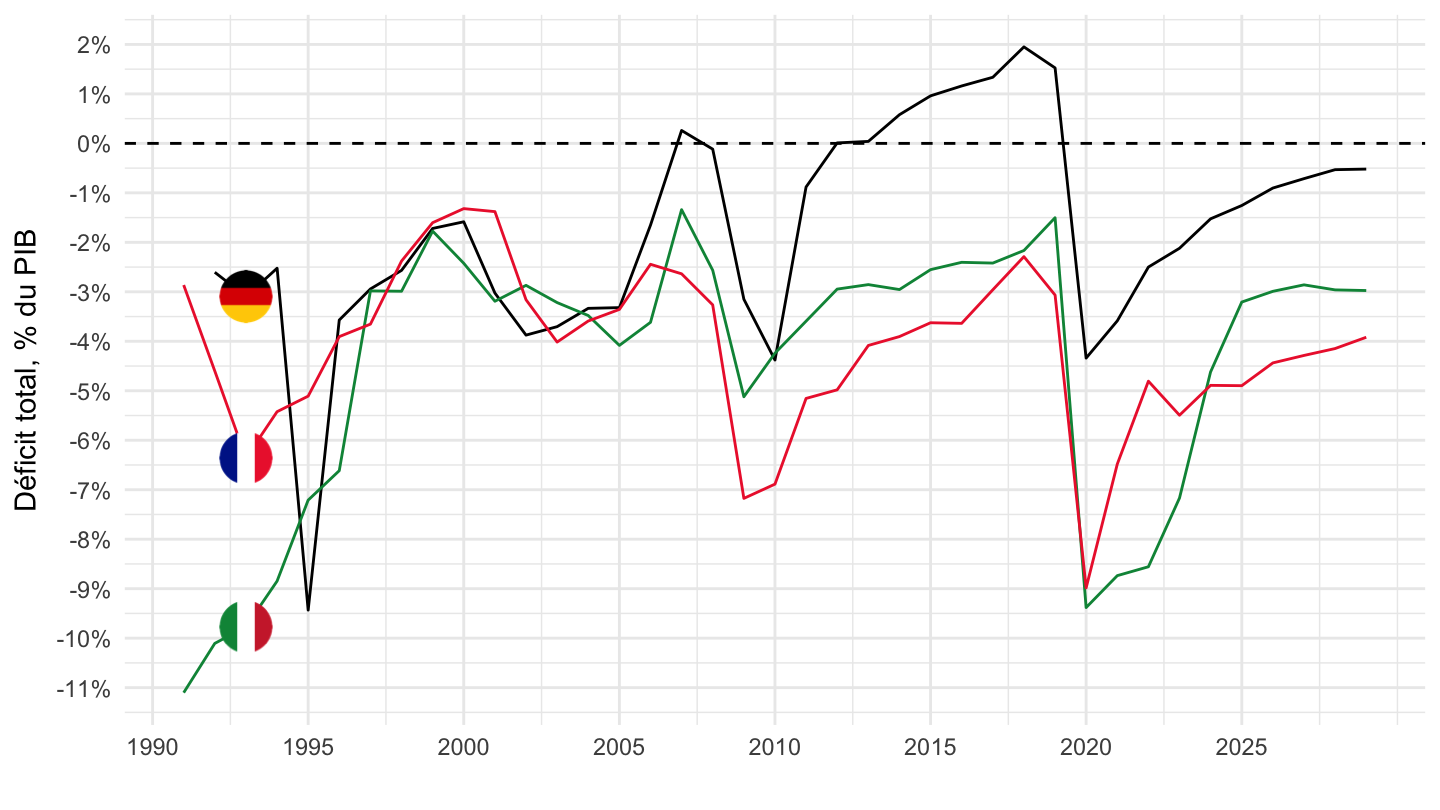
Net lending/borrowing - GGXCNL_G01_GDP_PT
Italy, France, Germany
Code
ig_d("imf", "GGXCNL_G01_GDP_PT", "IT-FR-DE")| Source | Dataset | PNG | |
|---|---|---|---|
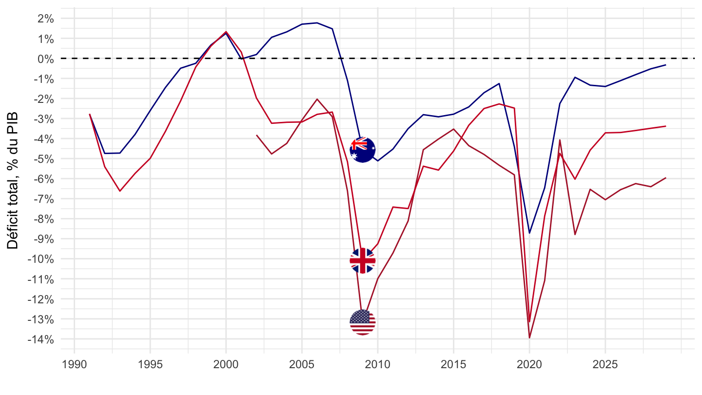
Australia, United Kingdom, United States
Code
ig_d("imf", "GGXCNL_G01_GDP_PT", "GB-US-AU")| Source | Dataset | PNG | |
|---|---|---|---|
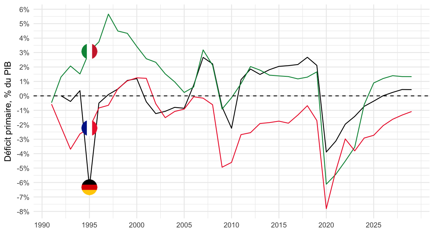
Primary net lending/borrowing - GGXONLB_G01_GDP_PT
Italy, France, Germany
Code
ig_d("imf", "GGXONLB_G01_GDP_PT", "IT-FR-DE")| Source | Dataset | PNG | |
|---|---|---|---|
Australia, United Kingdom, United States
Code
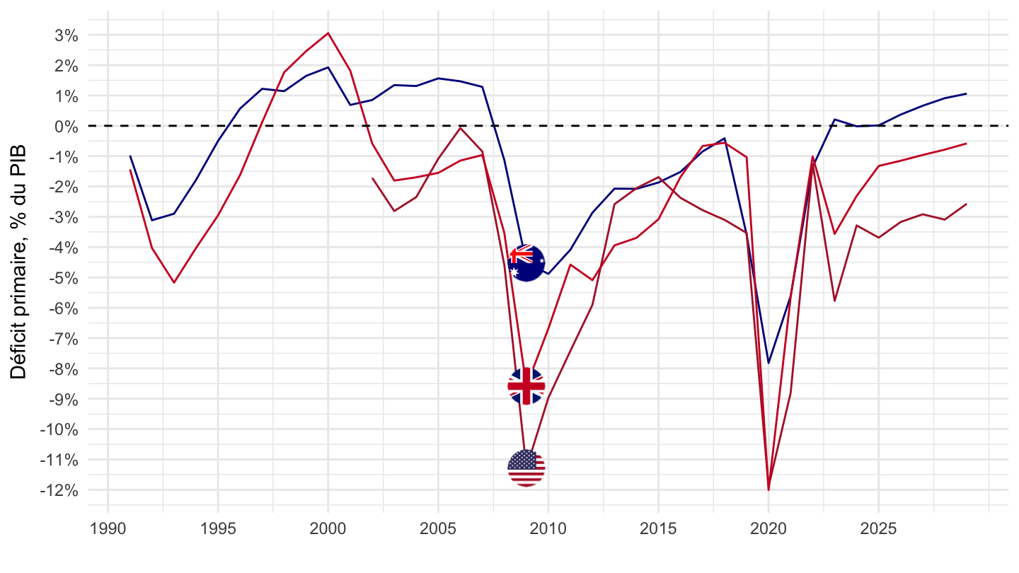
ig_d("imf", "GGXONLB_G01_GDP_PT", "GB-US-AU")| Source | Dataset | PNG | |
|---|---|---|---|
Cyclically adjusted primary balance (% of potential GDP)
Table
Code
FM |>
  filter(INDICATOR == "GGCBP_G01_PGDP_PT",
         date == as.Date("2018-01-01")) |>
  left_join(CL_AREA_FM |> rename(iso2c = AREA), by = "iso2c") |>
  select(iso2c, AREA_desc, value) |>
  arrange(-value) |>
  na.omit() %>%
  mutate_at(vars(3), funs(paste0(round(as.numeric(.), 1), " %"))) %>%
  {if (is_html_output()) datatable(., filter = 'top', rownames = F) else .}
Italy, France, Germany, United States
1990-
Code
FM |>
  filter(INDICATOR == "GGCBP_G01_PGDP_PT",
         iso2c %in% c("IT", "FR", "DE", "US", "GR", "ES"),
         date <= as.Date("2019-01-01")) |>
  left_join(CL_AREA_FM |> rename(iso2c = AREA), by = "iso2c") |>
  left_join(colors, by = c("AREA_desc" = "country")) |>
  mutate(value = value/100,
         color = ifelse(iso2c == "US", color2, color)) |>
  ggplot() +
  geom_line(aes(x = date, y = value, color = color)) +
  scale_color_identity() + theme_minimal() +
  geom_image(data = . %>%
               filter(date == as.Date("2013-01-01")) %>%
               mutate(image = paste0("../../icon/flag/", str_to_lower(gsub(" ", "-", AREA_desc)), ".png")),
             aes(x = date, y = value, image = image), asp = 1.5) +
  scale_x_date(breaks = seq(1920, 2100, 5) |> paste0("-01-01") |> as.Date(),
               labels = date_format("%Y")) +
  scale_y_continuous(breaks = 0.01*seq(-60, 60, 1),
                     labels = scales::percent_format(accuracy = 1)) +
  ylab("Cyclically adj. primary balance (% of potential GDP)") + xlab("")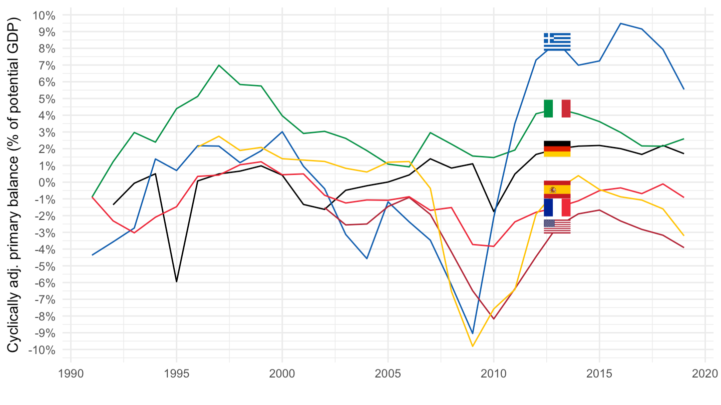
2005-
Code
FM |>
  filter(INDICATOR == "GGCBP_G01_PGDP_PT",
         iso2c %in% c("IT", "FR", "DE", "US", "GR", "ES"),
         date <= as.Date("2019-01-01"),
         date >= as.Date("2006-01-01")) |>
  left_join(CL_AREA_FM |> rename(iso2c = AREA), by = "iso2c") |>
  left_join(colors, by = c("AREA_desc" = "country")) |>
  mutate(value = value/100,
         color = ifelse(iso2c == "US", color2, color)) |>
  ggplot() +
  geom_line(aes(x = date, y = value, color = color)) +
  scale_color_identity() + theme_minimal() +
  geom_image(data = . %>%
               filter(date == as.Date("2013-01-01")) %>%
               mutate(image = paste0("../../icon/flag/", str_to_lower(gsub(" ", "-", AREA_desc)), ".png")),
             aes(x = date, y = value, image = image), asp = 1.5) +
  scale_x_date(breaks = seq(1920, 2100, 2) |> paste0("-01-01") |> as.Date(),
               labels = date_format("%Y")) +
  scale_y_continuous(breaks = 0.01*seq(-60, 60, 1),
                     labels = scales::percent_format(accuracy = 1)) +
  ylab("Cyclically adj. primary balance (% of potential GDP)") + xlab("")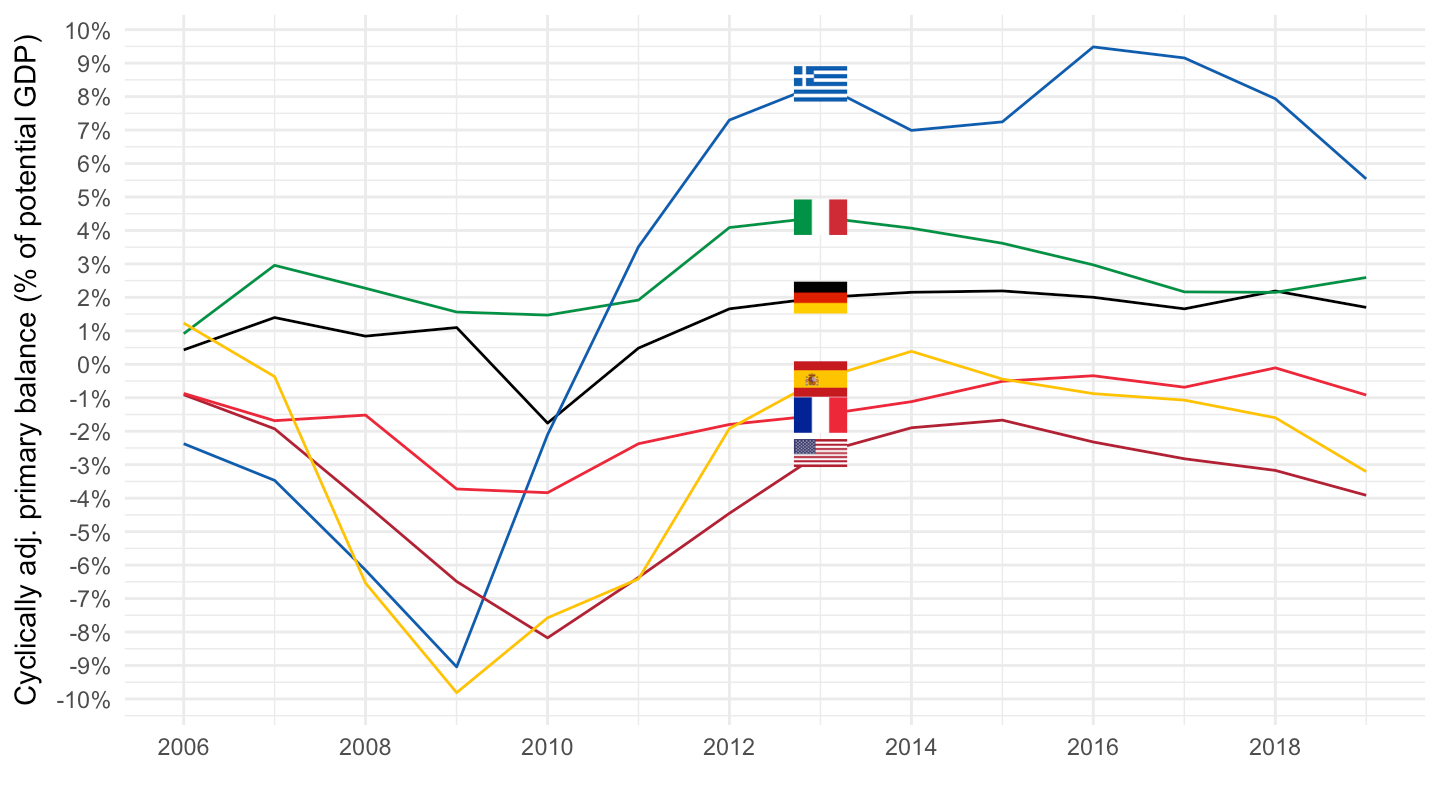
Denmark, Netherlands, Sweden
Code
FM |>
  filter(INDICATOR == "GGCBP_G01_PGDP_PT",
         iso2c %in% c("DK", "SE", "NL"),
         date <= as.Date("2019-01-01")) |>
  left_join(CL_AREA_FM |> rename(iso2c = AREA), by = "iso2c") |>
  left_join(colors, by = c("AREA_desc" = "country")) |>
  mutate(OBS_VALUE = value / 100,
         Counterpart_area = AREA_desc) |>
  ggplot() +
  geom_line(aes(x = date, y = OBS_VALUE, color = color)) +
  scale_color_identity() + theme_minimal() + add_flags +
  scale_x_date(breaks = seq(1920, 2100, 5) |> paste0("-01-01") |> as.Date(),
               labels = date_format("%Y")) +
  scale_y_continuous(breaks = 0.01*seq(-60, 60, 1),
                     labels = scales::percent_format(accuracy = 1)) +
  ylab("Cyclically adj. primary balance (% of potential GDP)") + xlab("")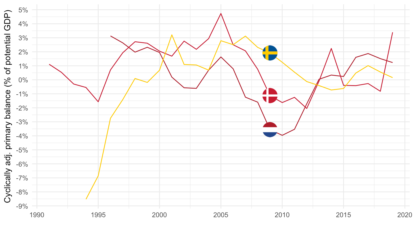
Germany, Italy, Netherlands
Code
FM |>
  filter(INDICATOR == "GGCBP_G01_PGDP_PT",
         iso2c %in% c("DE", "IT", "NL"),
         date >= as.Date("1995-01-01"),
         date <= as.Date("2019-01-01")) |>
  left_join(CL_AREA_FM |> rename(iso2c = AREA), by = "iso2c") |>
  left_join(colors, by = c("AREA_desc" = "country")) |>
  ggplot() +
  geom_line(aes(x = date, y = value/100, color = color)) +
  scale_color_identity() + theme_minimal() +
  geom_image(data = . %>%
               filter(date == as.Date("2010-01-01")) %>%
               mutate(image = paste0("../../icon/flag/", str_to_lower(gsub(" ", "-", AREA_desc)), ".png")),
             aes(x = date, y = value/100, image = image), asp = 1.5) +
  scale_x_date(breaks = seq(1920, 2100, 5) |> paste0("-01-01") |> as.Date(),
               labels = date_format("%Y")) +
  scale_y_continuous(breaks = 0.01*seq(-60, 60, 1),
                     labels = scales::percent_format(accuracy = 1)) +
  ylab("Cyclically adj. primary balance (% of potential GDP)") + xlab("")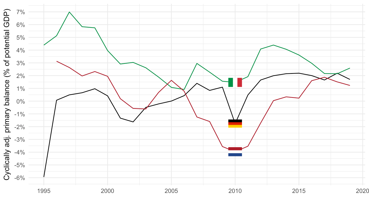
U.S., France, China
Code
FM |>
  filter(INDICATOR == "GGCBP_G01_PGDP_PT",
         iso2c %in% c("US", "FR", "CN"),
         date >= as.Date("1995-01-01"),
         date <= as.Date("2019-01-01")) |>
  left_join(CL_AREA_FM |> rename(iso2c = AREA), by = "iso2c") |>
  left_join(colors, by = c("AREA_desc" = "country")) |>
  ggplot() +
  geom_line(aes(x = date, y = value/100, color = color)) +
  scale_color_identity() + theme_minimal() +
  geom_image(data = . %>%
               filter(date == as.Date("2010-01-01")) %>%
               mutate(image = paste0("../../icon/flag/", str_to_lower(gsub(" ", "-", AREA_desc)), ".png")),
             aes(x = date, y = value/100, image = image), asp = 1.5) +
  scale_x_date(breaks = seq(1920, 2100, 5) |> paste0("-01-01") |> as.Date(),
               labels = date_format("%Y")) +
  scale_y_continuous(breaks = 0.01*seq(-60, 60, 1),
                     labels = scales::percent_format(accuracy = 1)) +
  ylab("Cyclically-Adjusted Primary Balance (CAPB)") + xlab("") +
  geom_hline(yintercept = 0, linetype = "dashed", color = "black")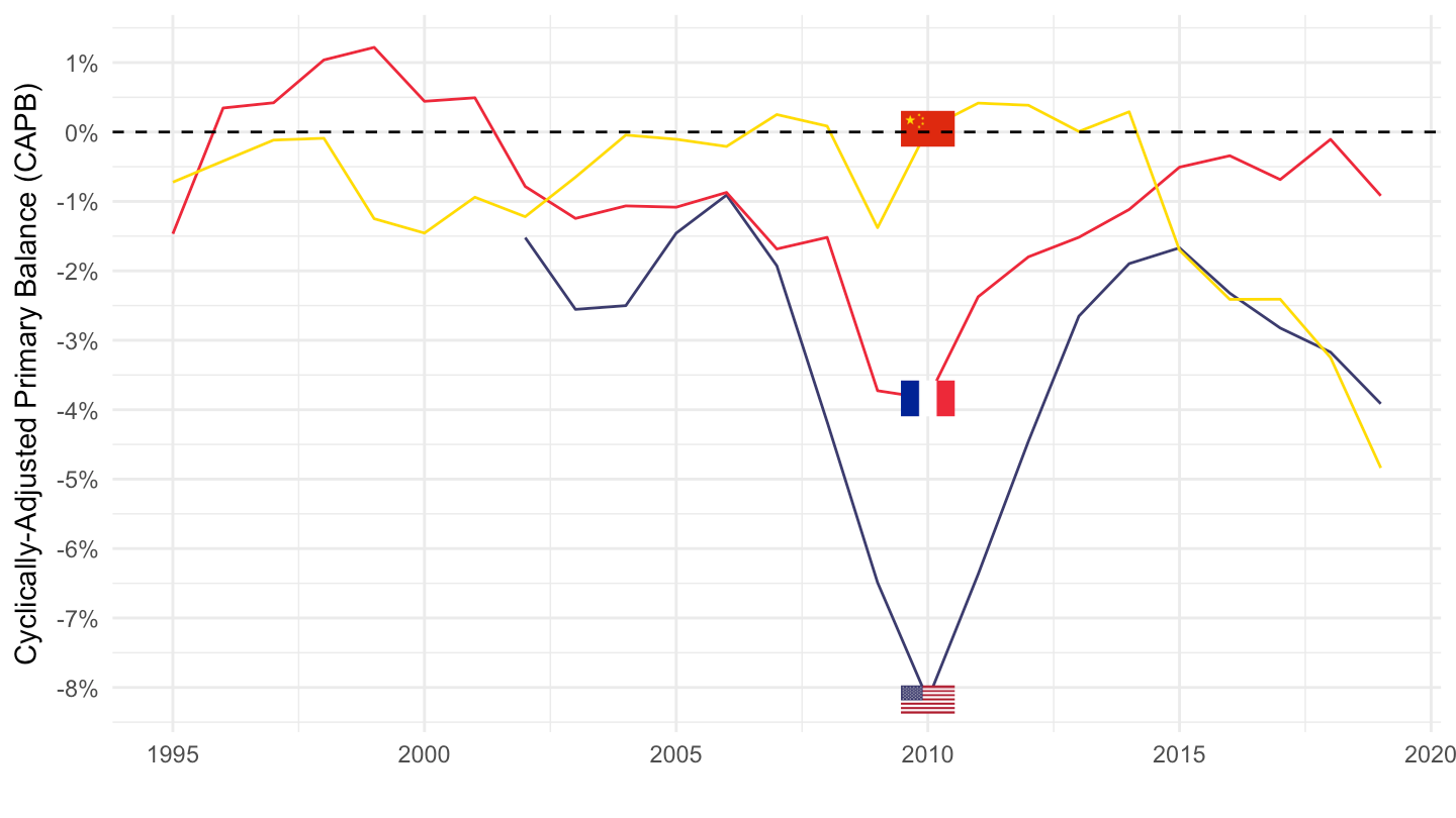
Netherlands, UK, Italy
Code
FM |>
  filter(INDICATOR == "GGCBP_G01_PGDP_PT",
         iso2c %in% c("NL", "GB", "IT"),
         date >= as.Date("1995-01-01"),
         date <= as.Date("2019-01-01")) |>
  left_join(CL_AREA_FM |> rename(iso2c = AREA), by = "iso2c") |>
  left_join(colors, by = c("AREA_desc" = "country")) |>
  mutate(value = value/100) |>
  ggplot() +
  geom_line(aes(x = date, y = value, color = color)) +
  scale_color_identity() + theme_minimal() +
  geom_image(data = . %>%
               filter(date == as.Date("2010-01-01")) %>%
               mutate(image = paste0("../../icon/flag/", str_to_lower(gsub(" ", "-", AREA_desc)), ".png")),
             aes(x = date, y = value, image = image), asp = 1.5) +
  scale_x_date(breaks = seq(1920, 2100, 5) |> paste0("-01-01") |> as.Date(),
               labels = date_format("%Y")) +
  scale_y_continuous(breaks = 0.01*seq(-60, 60, 1),
                     labels = scales::percent_format(accuracy = 1)) +
  ylab("Cyclically-Adjusted Primary Balance (CAPB)") + xlab("") +
  geom_hline(yintercept = 0, linetype = "dashed", color = "black")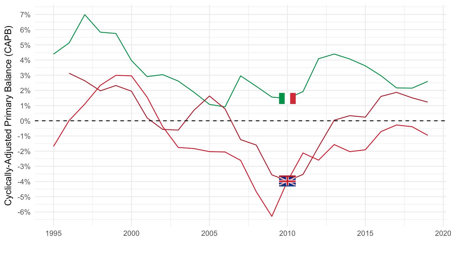
Austria, Poland, Switzerland
Code
FM |>
  filter(INDICATOR == "GGCBP_G01_PGDP_PT",
         iso2c %in% c("AT", "PL", "CH"),
         date >= as.Date("1995-01-01"),
         date <= as.Date("2019-01-01")) |>
  left_join(CL_AREA_FM |> rename(iso2c = AREA), by = "iso2c") |>
  left_join(colors, by = c("AREA_desc" = "country")) |>
  mutate(value = value/100) |>
  ggplot() +
  geom_line(aes(x = date, y = value, color = color)) +
  scale_color_identity() + theme_minimal() +
  geom_image(data = . %>%
               filter(date == as.Date("2010-01-01")) %>%
               mutate(image = paste0("../../icon/flag/", str_to_lower(gsub(" ", "-", AREA_desc)), ".png")),
             aes(x = date, y = value, image = image), asp = 1.5) +
  scale_x_date(breaks = seq(1920, 2100, 5) |> paste0("-01-01") |> as.Date(),
               labels = date_format("%Y")) +
  scale_y_continuous(breaks = 0.01*seq(-60, 60, 1),
                     labels = scales::percent_format(accuracy = 1)) +
  ylab("Cyclically-Adjusted Primary Balance (CAPB)") + xlab("") +
  geom_hline(yintercept = 0, linetype = "dashed", color = "black")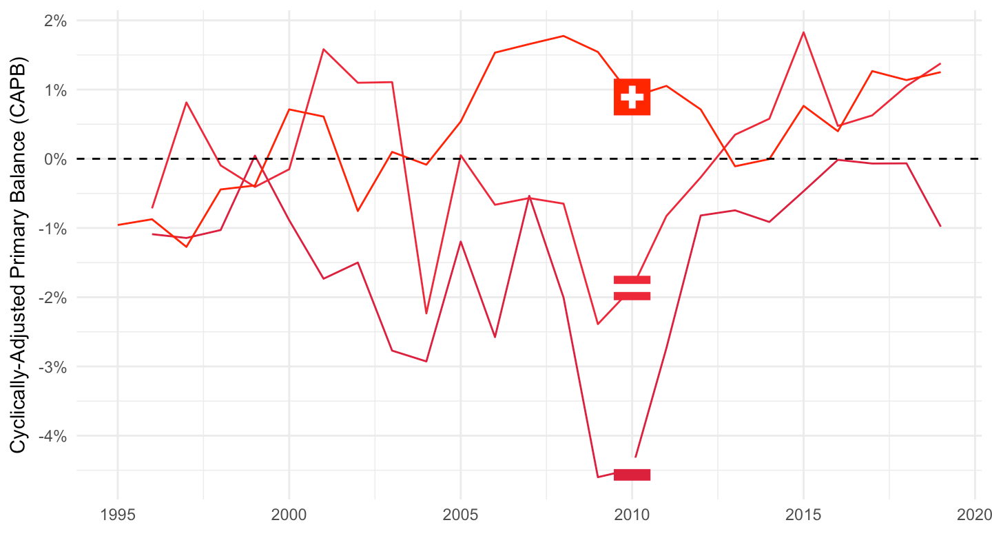
Belgium, Spain, Czechia
Code
FM |>
  filter(INDICATOR == "GGCBP_G01_PGDP_PT",
         iso2c %in% c("BE", "ES", "CZ"),
         date >= as.Date("1995-01-01"),
         date <= as.Date("2019-01-01")) |>
  left_join(CL_AREA_FM |> rename(iso2c = AREA), by = "iso2c") |>
  left_join(colors, by = c("AREA_desc" = "country")) |>
  ggplot() +
  geom_line(aes(x = date, y = value/100, color = color)) +
  scale_color_identity() + theme_minimal() +
  geom_image(data = . %>%
               filter(date == as.Date("2010-01-01")) %>%
               mutate(image = paste0("../../icon/flag/", str_to_lower(gsub(" ", "-", AREA_desc)), ".png")),
             aes(x = date, y = value/100, image = image), asp = 1.5) +
  scale_x_date(breaks = seq(1920, 2100, 5) |> paste0("-01-01") |> as.Date(),
               labels = date_format("%Y")) +
  scale_y_continuous(breaks = 0.01*seq(-60, 60, 1),
                     labels = scales::percent_format(accuracy = 1)) +
  ylab("Cyclically-Adjusted Primary Balance (CAPB)") + xlab("") +
  geom_hline(yintercept = 0, linetype = "dashed", color = "black")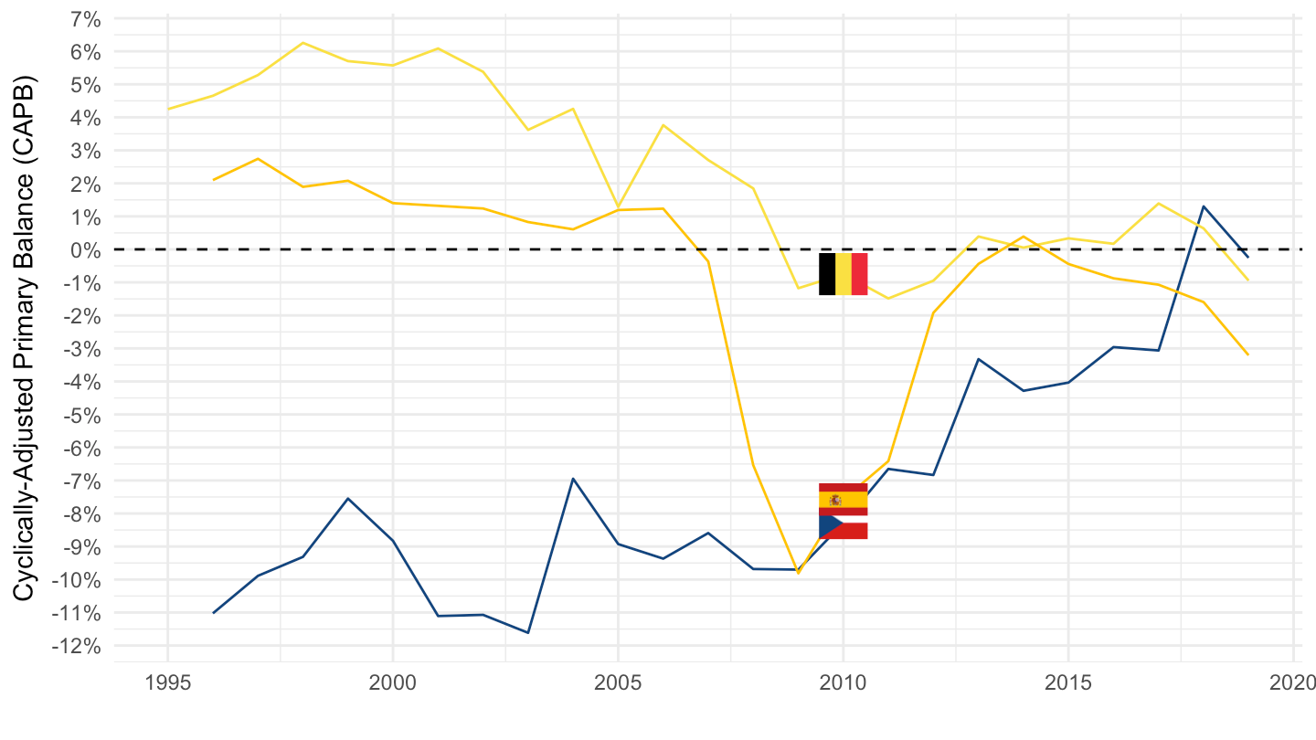
Cyclically adjusted balance (% of potential GDP)
Table
Code
FM |>
  filter(INDICATOR == "GGCB_G01_PGDP_PT",
         date == as.Date("2018-01-01")) |>
  left_join(CL_AREA_FM |> rename(iso2c = AREA), by = "iso2c") |>
  select(iso2c, AREA_desc, value) |>
  arrange(-value) |>
  na.omit() %>%
  mutate_at(vars(3), funs(paste0(round(as.numeric(.), 1), " %"))) %>%
  {if (is_html_output()) datatable(., filter = 'top', rownames = F) else .}
Italy, France, Germany, United States
Code
FM |>
  filter(INDICATOR == "GGCB_G01_PGDP_PT",
         iso2c %in% c("IT", "FR", "DE", "US"),
         date <= as.Date("2019-01-01")) |>
  left_join(CL_AREA_FM |> rename(iso2c = AREA), by = "iso2c") |>
  left_join(colors, by = c("AREA_desc" = "country")) |>
  ggplot() +
  geom_line(aes(x = date, y = value/100, color = color)) +
  scale_color_identity() + theme_minimal() +
  geom_image(data = . %>%
               filter(date == as.Date("2017-01-01")) %>%
               mutate(image = paste0("../../icon/flag/", str_to_lower(gsub(" ", "-", AREA_desc)), ".png")),
             aes(x = date, y = value/100, image = image), asp = 1.5) +
  scale_x_date(breaks = seq(1920, 2100, 5) |> paste0("-01-01") |> as.Date(),
               labels = date_format("%Y")) +
  scale_y_continuous(breaks = 0.01*seq(-60, 60, 1),
                     labels = scales::percent_format(accuracy = 1)) +
  ylab("Cyclically adj. balance (% of potential GDP)") + xlab("")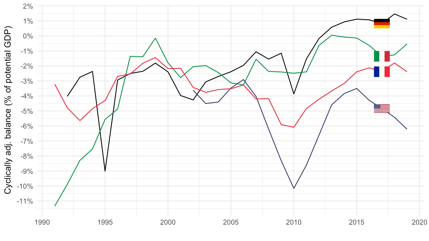
Denmark, Netherlands, Sweden
Code
FM |>
  filter(INDICATOR == "GGCB_G01_PGDP_PT",
         iso2c %in% c("DK", "SE", "NL"),
         date <= as.Date("2019-01-01")) |>
  left_join(CL_AREA_FM |> rename(iso2c = AREA), by = "iso2c") |>
  left_join(colors, by = c("AREA_desc" = "country")) |>
  ggplot() +
  geom_line(aes(x = date, y = value/100, color = color)) +
  scale_color_identity() + theme_minimal() +
  geom_image(data = . %>%
               filter(date == as.Date("2010-01-01")) %>%
               mutate(image = paste0("../../icon/flag/", str_to_lower(gsub(" ", "-", AREA_desc)), ".png")),
             aes(x = date, y = value/100, image = image), asp = 1.5) +
  scale_x_date(breaks = seq(1920, 2100, 5) |> paste0("-01-01") |> as.Date(),
               labels = date_format("%Y")) +
  scale_y_continuous(breaks = 0.01*seq(-60, 60, 1),
                     labels = scales::percent_format(accuracy = 1)) +
  ylab("Cyclically adj. balance (% of potential GDP)") + xlab("")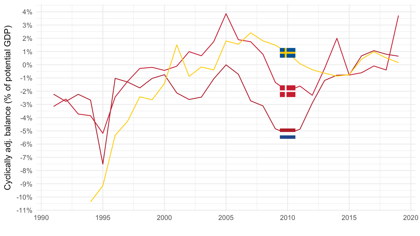
Germany, Italy, Netherlands
Code
FM |>
  filter(INDICATOR == "GGCB_G01_PGDP_PT",
         iso2c %in% c("DE", "IT", "NL"),
         date >= as.Date("1995-01-01"),
         date <= as.Date("2019-01-01")) |>
  left_join(CL_AREA_FM |> rename(iso2c = AREA), by = "iso2c") |>
  left_join(colors, by = c("AREA_desc" = "country")) |>
  ggplot() +
  geom_line(aes(x = date, y = value/100, color = color)) +
  scale_color_identity() + theme_minimal() +
  geom_image(data = . %>%
               filter(date == as.Date("2010-01-01")) %>%
               mutate(image = paste0("../../icon/flag/", str_to_lower(gsub(" ", "-", AREA_desc)), ".png")),
             aes(x = date, y = value/100, image = image), asp = 1.5) +
  scale_x_date(breaks = seq(1920, 2100, 5) |> paste0("-01-01") |> as.Date(),
               labels = date_format("%Y")) +
  scale_y_continuous(breaks = 0.01*seq(-60, 60, 1),
                     labels = scales::percent_format(accuracy = 1)) +
  ylab("Cyclically adj. balance (% of potential GDP)") + xlab("")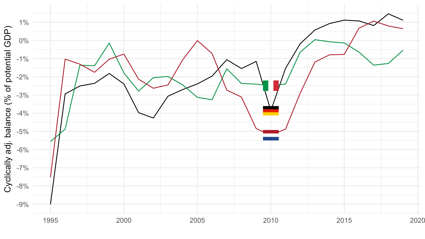
Germany: Average Demand of Main Trading Partners
Germany
Code
FM |>
  filter(INDICATOR == "GGCB_G01_PGDP_PT",
         date >= as.Date("1995-01-01"),
         date <= as.Date("2020-01-01")) |>
  select(iso2c, date, value) |>
  inner_join(WTS |>
              mutate(date = paste0(TIME_PERIOD, "-01-01") |> as.Date()) |>
              filter(REF_AREA == "DE",
                     TRADE_WEIGHT == "O", # Overall trade weight
                     CURRENCY_TRANS == "H10", # Euro area-19 countries and EER-38 group of trading partners
                     date == as.Date("1995-01-01")) |>
              select(iso2c = COUNT_AREA, share_1995 = OBS_VALUE) |>
               mutate(share_1995 = share_1995/sum(share_1995)),
            by = "iso2c") |>
  inner_join(WTS |>
              mutate(date = paste0(TIME_PERIOD, "-01-01") |> as.Date()) |>
              filter(REF_AREA == "DE",
                     TRADE_WEIGHT == "O", # Overall trade weight
                     CURRENCY_TRANS == "H10", # Euro area-19 countries and EER-38 group of trading partners
                     date == as.Date("2015-01-01")) |>
              select(iso2c = COUNT_AREA, share_2015 = OBS_VALUE) |>
               mutate(share_2015 = share_2015/sum(share_2015)),
            by = "iso2c") |>
  group_by(date) |>
  summarise(`Germany's Partners CAPB (1995 shares)` = sum(share_1995*value),
            `Germany's Partners CAPB (2015 shares)` = sum(share_2015*value)) |>
  left_join(FM |>
              filter(INDICATOR == "GGCBP_G01_PGDP_PT",
                     iso2c %in% c("DE"),
                     date >= as.Date("1995-01-01"),
                     date <= as.Date("2019-01-01")) |>
              select(date, `Germany's CAPB` = value),
            by = "date") |>
  gather(variable, value, -date) |>
  ggplot() +
  geom_line(aes(x = date, y = value/100, color = variable, linetype = variable)) +
  scale_color_manual(values = viridis(5)[1:4]) +
  theme_minimal() +
  scale_x_date(breaks = seq(1920, 2100, 5) |> paste0("-01-01") |> as.Date(),
               labels = date_format("%Y")) +
  theme(legend.position = c(0.3, 0.9),
        legend.title = element_blank()) +
  scale_y_continuous(breaks = 0.01*seq(-60, 60, 1),
                     labels = scales::percent_format(accuracy = 1)) +
  ylab("Cyclically-Adjusted Primary Balance (CAPB)") + xlab("") +
  geom_hline(yintercept = 0, linetype = "dashed", color = "black")