| source | dataset | Title | .html | .rData |
|---|---|---|---|---|
| insee | t_conso_val | Dépenses de consommation des ménages aux prix courants (données CVS-CJO) | 2026-07-23 | 2026-02-27 |
Dépenses de consommation des ménages aux prix courants (données CVS-CJO)
Données - INSEE
Info
Données sur la macroéconomie en France
| source | dataset | Title | .html | .rData |
|---|---|---|---|---|
| bdf | CFT | Comptes Financiers Trimestriels | 2026-07-23 | 2025-03-09 |
| insee | CNA-2014-CONSO-SI | Dépenses de consommation finale par secteur institutionnel | 2026-07-23 | 2026-07-23 |
| insee | CNA-2014-CSI | Comptes des secteurs institutionnels | 2026-07-23 | 2026-07-23 |
| insee | CNA-2014-FBCF-BRANCHE | Formation brute de capital fixe (FBCF) par branche | 2026-07-23 | 2026-07-23 |
| insee | CNA-2014-FBCF-SI | Formation brute de capital fixe (FBCF) par secteur institutionnel | 2026-07-23 | 2026-07-23 |
| insee | CNA-2014-RDB | Revenu et pouvoir d’achat des ménages | 2026-07-23 | 2026-07-23 |
| insee | CNA-2020-CONSO-MEN | Consommation des ménages | 2026-07-23 | 2026-07-23 |
| insee | CNA-2020-PIB | Produit intérieur brut (PIB) et ses composantes | 2026-07-23 | 2026-07-23 |
| insee | CNT-2014-CB | Comptes des branches | 2026-07-23 | 2026-07-23 |
| insee | CNT-2014-CSI | Comptes de secteurs institutionnels | 2026-07-23 | 2026-07-22 |
| insee | CNT-2014-OPERATIONS | Opérations sur biens et services | 2026-07-23 | 2026-07-23 |
| insee | CNT-2014-PIB-EQB-RF | Équilibre du produit intérieur brut | 2026-07-23 | 2026-07-23 |
| insee | CONSO-MENAGES-2020 | Consommation des ménages en biens | 2026-07-23 | 2026-07-23 |
| insee | ICA-2015-IND-CONS | Indices de chiffre d'affaires dans l'industrie et la construction | 2026-07-23 | 2026-07-23 |
| insee | conso-mensuelle | Consommation de biens, données mensuelles | 2026-07-23 | 2023-07-04 |
| insee | t_1101 | 1.101 – Le produit intérieur brut et ses composantes à prix courants (En milliards d'euros) | 2026-07-23 | 2022-01-02 |
| insee | t_1102 | 1.102 – Le produit intérieur brut et ses composantes en volume aux prix de l'année précédente chaînés (En milliards d'euros 2014) | 2026-07-23 | 2020-10-30 |
| insee | t_1105 | 1.105 – Produit intérieur brut - les trois approches à prix courants (En milliards d'euros) - t_1105 | 2026-07-23 | 2020-10-30 |
LAST_COMPILE
| LAST_COMPILE |
|---|
| 2026-07-24 |
variable
Code
t_conso_val %>%
  left_join(variable, by = "variable") %>%
  group_by(variable, Variable) %>%
  summarise(Nobs = n()) %>%
  arrange(-Nobs) %>%
print_table_conditional| variable | Variable | Nobs |
|---|---|---|
| (CHTR) | Correction territoriale | 308 |
| (DE) à (C5) | Industrie | 308 |
| (FZ) à (RU) | Total services | 308 |
| (GZ) à (MN), (RU) | Services marchands | 308 |
| AZ | Produits agricoles | 308 |
| C | Produits manufacturés | 308 |
| C1 | Produits agro-alimentaires | 308 |
| C2 | Cokéfaction et raffinage | 308 |
| C3 | Biens d'équipement | 308 |
| C4 | Matériels de transport | 308 |
| C5 | Autres produits industriels | 308 |
| DE | Energie, eau, déchets | 308 |
| FZ | Construction | 308 |
| GZ | Commerce | 308 |
| HZ | Transport | 308 |
| IZ | Hébergement-restauration | 308 |
| JZ | Information-communication | 308 |
| KZ | Services financiers | 308 |
| LZ | Services immobiliers | 308 |
| MN | Services aux entreprises | 308 |
| OQ | Services non marchands | 308 |
| RU | Services aux ménages | 308 |
| TOTAL | Total | 308 |
date
Code
t_conso_val %>%
  group_by(date) %>%
  summarise(Nobs = n()) %>%
  arrange(desc(date)) %>%
  print_table_conditional
Evolution
2017T2-
Code
t_conso_val %>%
  left_join(variable, by = "variable") %>%
  filter(date %in% c(max(date), as.Date("2017-04-01"))) %>%
  spread(date, value) %>%
  mutate(change = round(100*(.[[4]]/.[[3]]-1), 2)) %>%
  arrange(-change) %>%
print_table_conditional(.)| variable | Variable | 2017-04-01 | 2025-10-01 | change |
|---|---|---|---|---|
| (CHTR) | Correction territoriale | -2.454 | -5.057 | 106.07 |
| KZ | Services financiers | 17.969 | 32.073 | 78.49 |
| IZ | Hébergement-restauration | 20.957 | 34.400 | 64.15 |
| MN | Services aux entreprises | 7.385 | 11.774 | 59.43 |
| GZ | Commerce | 1.145 | 1.689 | 47.51 |
| RU | Services aux ménages | 11.284 | 16.384 | 45.20 |
| DE | Energie, eau, déchets | 13.198 | 19.077 | 44.54 |
| (GZ) à (MN), (RU) | Services marchands | 141.924 | 201.631 | 42.07 |
| HZ | Transport | 9.590 | 13.574 | 41.54 |
| FZ | Construction | 5.370 | 7.568 | 40.93 |
| (FZ) à (RU) | Total services | 163.144 | 228.645 | 40.15 |
| TOTAL | Total | 297.736 | 388.447 | 30.47 |
| LZ | Services immobiliers | 62.418 | 78.156 | 25.21 |
| C1 | Produits agro-alimentaires | 42.304 | 52.673 | 24.51 |
| AZ | Produits agricoles | 7.542 | 9.379 | 24.36 |
| OQ | Services non marchands | 15.850 | 19.446 | 22.69 |
| JZ | Information-communication | 11.177 | 13.582 | 21.52 |
| (DE) à (C5) | Industrie | 129.503 | 155.479 | 20.06 |
| C2 | Cokéfaction et raffinage | 11.658 | 13.788 | 18.27 |
| C | Produits manufacturés | 116.305 | 136.403 | 17.28 |
| C4 | Matériels de transport | 16.387 | 18.981 | 15.83 |
| C5 | Autres produits industriels | 37.028 | 41.289 | 11.51 |
| C3 | Biens d'équipement | 8.929 | 9.670 | 8.30 |
2019T4-
Code
t_conso_val %>%
  left_join(variable, by = "variable") %>%
  filter(date %in% c(max(date), as.Date("2019-10-01"))) %>%
  spread(date, value) %>%
  mutate(change = round(100*(.[[4]]/.[[3]]-1), 2)) %>%
  arrange(change) %>%
print_table_conditional(.)| variable | Variable | 2019-10-01 | 2025-10-01 | change |
|---|---|---|---|---|
| C2 | Cokéfaction et raffinage | 13.193 | 13.788 | 4.51 |
| C3 | Biens d'équipement | 9.182 | 9.670 | 5.31 |
| C4 | Matériels de transport | 17.761 | 18.981 | 6.87 |
| C5 | Autres produits industriels | 37.738 | 41.289 | 9.41 |
| C | Produits manufacturés | 122.189 | 136.403 | 11.63 |
| (DE) à (C5) | Industrie | 136.271 | 155.479 | 14.10 |
| JZ | Information-communication | 11.855 | 13.582 | 14.57 |
| AZ | Produits agricoles | 8.058 | 9.379 | 16.39 |
| OQ | Services non marchands | 16.590 | 19.446 | 17.22 |
| LZ | Services immobiliers | 66.061 | 78.156 | 18.31 |
| C1 | Produits agro-alimentaires | 44.314 | 52.673 | 18.86 |
| TOTAL | Total | 317.815 | 388.447 | 22.22 |
| GZ | Commerce | 1.324 | 1.689 | 27.57 |
| (FZ) à (RU) | Total services | 176.506 | 228.645 | 29.54 |
| FZ | Construction | 5.836 | 7.568 | 29.68 |
| (GZ) à (MN), (RU) | Services marchands | 154.080 | 201.631 | 30.86 |
| RU | Services aux ménages | 12.520 | 16.384 | 30.86 |
| HZ | Transport | 10.198 | 13.574 | 33.10 |
| DE | Energie, eau, déchets | 14.082 | 19.077 | 35.47 |
| MN | Services aux entreprises | 8.434 | 11.774 | 39.60 |
| IZ | Hébergement-restauration | 24.626 | 34.400 | 39.69 |
| (CHTR) | Correction territoriale | -3.020 | -5.057 | 67.45 |
| KZ | Services financiers | 19.061 | 32.073 | 68.27 |
2 years
Code
t_conso_val %>%
  left_join(variable, by = "variable") %>%
  filter(date %in% c(max(date), max(date) - years(2))) %>%
  spread(date, value) %>%
  mutate(change = round(100*(.[[4]]/.[[3]]-1), 2)) %>%
  arrange(-change) %>%
print_table_conditional(.)| variable | Variable | 2023-10-01 | 2025-10-01 | change |
|---|---|---|---|---|
| (CHTR) | Correction territoriale | -3.385 | -5.057 | 49.39 |
| MN | Services aux entreprises | 10.748 | 11.774 | 9.55 |
| IZ | Hébergement-restauration | 31.469 | 34.400 | 9.31 |
| HZ | Transport | 12.432 | 13.574 | 9.19 |
| RU | Services aux ménages | 15.182 | 16.384 | 7.92 |
| DE | Energie, eau, déchets | 17.744 | 19.077 | 7.51 |
| LZ | Services immobiliers | 73.277 | 78.156 | 6.66 |
| (GZ) à (MN), (RU) | Services marchands | 190.236 | 201.631 | 5.99 |
| (FZ) à (RU) | Total services | 216.175 | 228.645 | 5.77 |
| OQ | Services non marchands | 18.573 | 19.446 | 4.70 |
| GZ | Commerce | 1.637 | 1.689 | 3.18 |
| TOTAL | Total | 376.461 | 388.447 | 3.18 |
| FZ | Construction | 7.365 | 7.568 | 2.76 |
| AZ | Produits agricoles | 9.132 | 9.379 | 2.70 |
| C5 | Autres produits industriels | 40.754 | 41.289 | 1.31 |
| JZ | Information-communication | 13.456 | 13.582 | 0.94 |
| C3 | Biens d'équipement | 9.604 | 9.670 | 0.69 |
| (DE) à (C5) | Industrie | 154.540 | 155.479 | 0.61 |
| C1 | Produits agro-alimentaires | 52.403 | 52.673 | 0.52 |
| KZ | Services financiers | 32.035 | 32.073 | 0.12 |
| C | Produits manufacturés | 136.796 | 136.403 | -0.29 |
| C4 | Matériels de transport | 19.271 | 18.981 | -1.50 |
| C2 | Cokéfaction et raffinage | 14.765 | 13.788 | -6.62 |
Last year
Code
t_conso_val %>%
  left_join(variable, by = "variable") %>%
  filter(date %in% c(max(date), max(date) - years(1))) %>%
  spread(date, value) %>%
  mutate(change = round(100*(.[[4]]/.[[3]]-1), 2)) %>%
  arrange(-change) %>%
print_table_conditional(.)| variable | Variable | 2024-10-01 | 2025-10-01 | change |
|---|---|---|---|---|
| (CHTR) | Correction territoriale | -3.760 | -5.057 | 34.49 |
| KZ | Services financiers | 29.624 | 32.073 | 8.27 |
| MN | Services aux entreprises | 11.368 | 11.774 | 3.57 |
| (GZ) à (MN), (RU) | Services marchands | 195.055 | 201.631 | 3.37 |
| (FZ) à (RU) | Total services | 221.553 | 228.645 | 3.20 |
| GZ | Commerce | 1.637 | 1.689 | 3.18 |
| LZ | Services immobiliers | 75.821 | 78.156 | 3.08 |
| IZ | Hébergement-restauration | 33.428 | 34.400 | 2.91 |
| AZ | Produits agricoles | 9.162 | 9.379 | 2.37 |
| OQ | Services non marchands | 19.058 | 19.446 | 2.04 |
| HZ | Transport | 13.304 | 13.574 | 2.03 |
| RU | Services aux ménages | 16.085 | 16.384 | 1.86 |
| FZ | Construction | 7.440 | 7.568 | 1.72 |
| TOTAL | Total | 383.080 | 388.447 | 1.40 |
| C3 | Biens d'équipement | 9.564 | 9.670 | 1.11 |
| C5 | Autres produits industriels | 40.855 | 41.289 | 1.06 |
| C | Produits manufacturés | 136.045 | 136.403 | 0.26 |
| C1 | Produits agro-alimentaires | 52.579 | 52.673 | 0.18 |
| (DE) à (C5) | Industrie | 156.125 | 155.479 | -0.41 |
| C4 | Matériels de transport | 19.108 | 18.981 | -0.66 |
| C2 | Cokéfaction et raffinage | 13.939 | 13.788 | -1.08 |
| JZ | Information-communication | 13.789 | 13.582 | -1.50 |
| DE | Energie, eau, déchets | 20.080 | 19.077 | -5.00 |
Consommation, Services financiers
2017-
Code
t_conso_val %>%
  filter(variable %in% c("AZ", "C1", "KZ"),
         date >= as.Date("2017-01-01")) %>%
  group_by(variable) %>%
  arrange(date) %>%
  mutate(value = 100*value/value[1]) %>%
  left_join(variable, by = "variable") %>%
  ggplot + geom_line(aes(x = date, y = value, color = Variable)) +
  theme_minimal() + ylab("Consommation trimestrielle") + xlab("") +
  theme(legend.title = element_blank(),
        legend.position = c(0.2, 0.8)) +
  scale_x_date(breaks = seq(1950, 2100, 1) %>% paste0("-01-01") %>% as.Date,
               labels = date_format("%Y")) +
  scale_y_log10(breaks = seq(70, 1000, 5))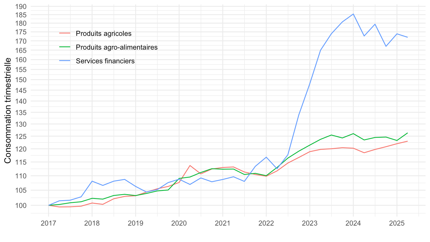
Produits agricoles
1949-
Code
t_conso_val %>%
  filter(variable %in% c("AZ")) %>%
  group_by(variable) %>%
  arrange(date) %>%
  mutate(value = 100*value/value[1]) %>%
  left_join(variable, by = "variable") %>%
  ggplot + geom_line(aes(x = date, y = value)) +
  theme_minimal() + ylab("Consommation trimestrielle de produits agricoles") + xlab("") +
  theme(legend.title = element_blank(),
        legend.position = c(0.2, 0.9)) +
  scale_x_date(breaks = seq(1950, 2100, 5) %>% paste0("-01-01") %>% as.Date,
               labels = date_format("%Y")) +
  scale_y_log10(breaks = c(100, 200, 500, 800, 1000, 2000, 5000, 10000))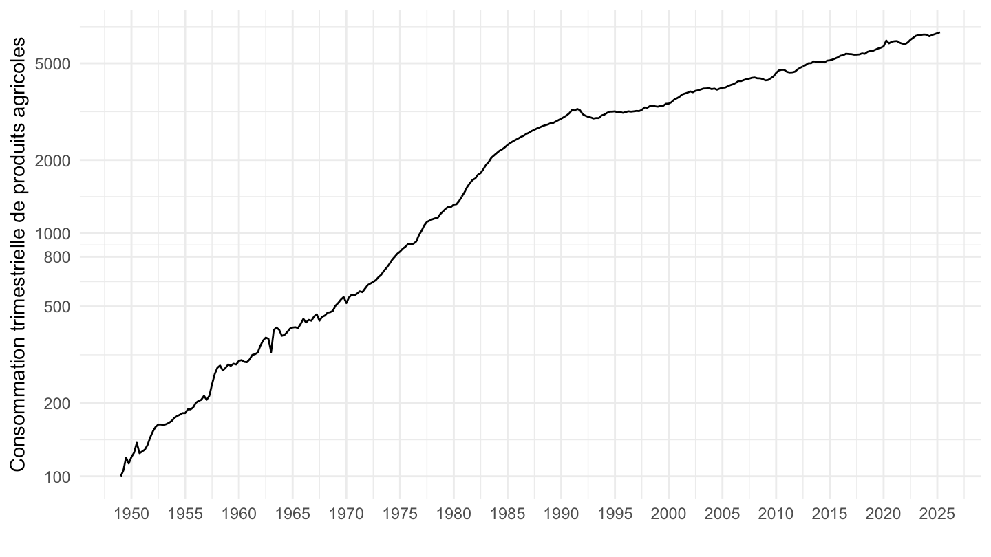
Consommation alimentaire
1949-
Code
t_conso_val %>%
  filter(variable %in% c("AZ", "C1")) %>%
  group_by(variable) %>%
  arrange(date) %>%
  mutate(value = 100*value/value[1]) %>%
  left_join(variable, by = "variable") %>%
  ggplot + geom_line(aes(x = date, y = value, color = Variable)) +
  theme_minimal() + ylab("Consommation trimestrielle") + xlab("") +
  theme(legend.title = element_blank(),
        legend.position = c(0.2, 0.8)) +
  scale_x_date(breaks = seq(1950, 2100, 5) %>% paste0("-01-01") %>% as.Date,
               labels = date_format("%Y")) +
  scale_y_log10(breaks = c(100, 200, 500, 800, 1000, 2000, 5000, 10000))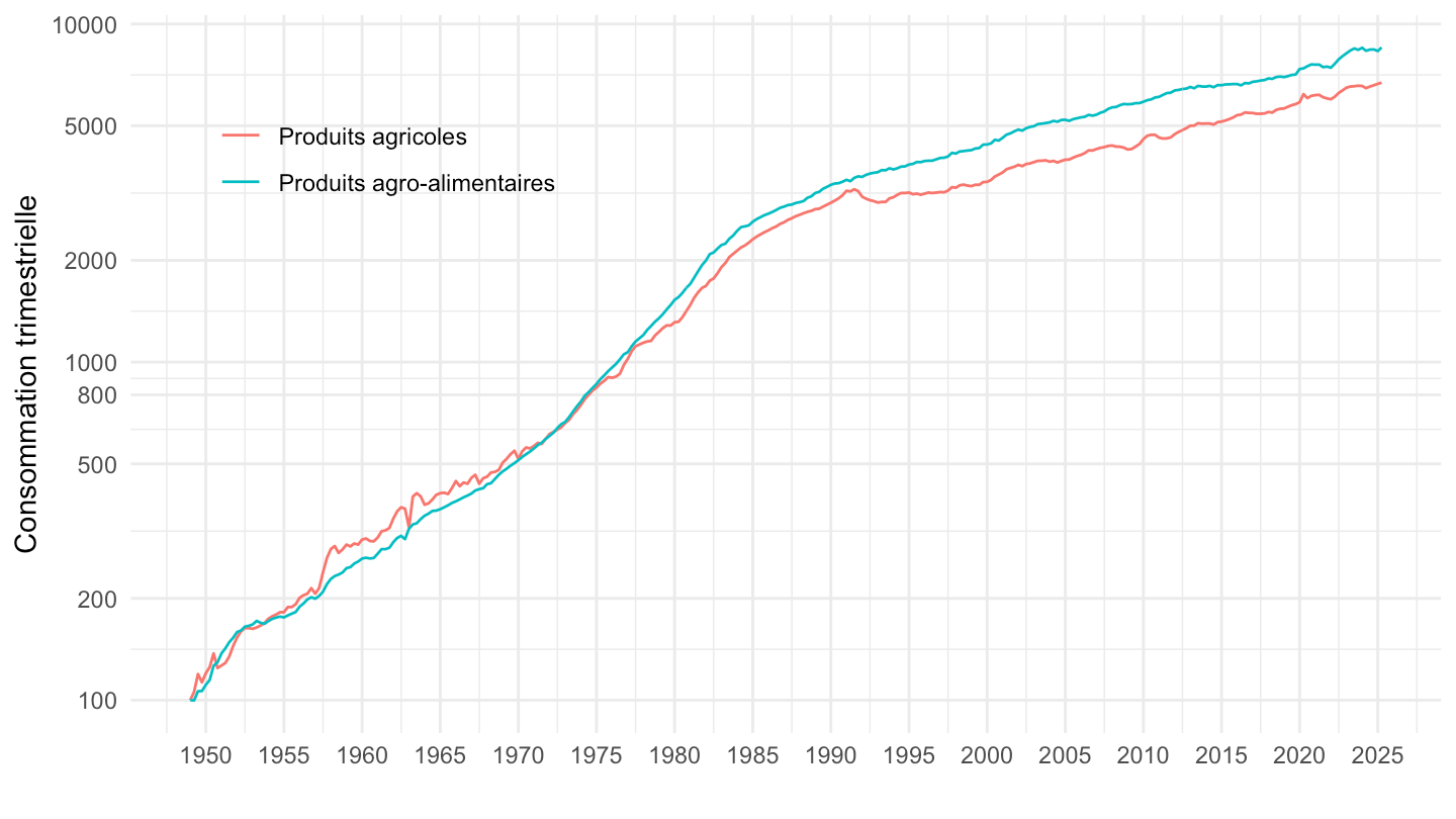
2010-
Code
t_conso_val %>%
  filter(variable %in% c("AZ", "C1"),
         date >= as.Date("2010-01-01")) %>%
  group_by(variable) %>%
  arrange(date) %>%
  mutate(value = 100*value/value[1]) %>%
  left_join(variable, by = "variable") %>%
  ggplot + geom_line(aes(x = date, y = value, color = Variable)) +
  theme_minimal() + ylab("Consommation trimestrielle") + xlab("") +
  theme(legend.title = element_blank(),
        legend.position = c(0.2, 0.8)) +
  scale_x_date(breaks = seq(1950, 2100, 1) %>% paste0("-01-01") %>% as.Date,
               labels = date_format("%Y")) +
  scale_y_log10(breaks = seq(70, 1000, 5))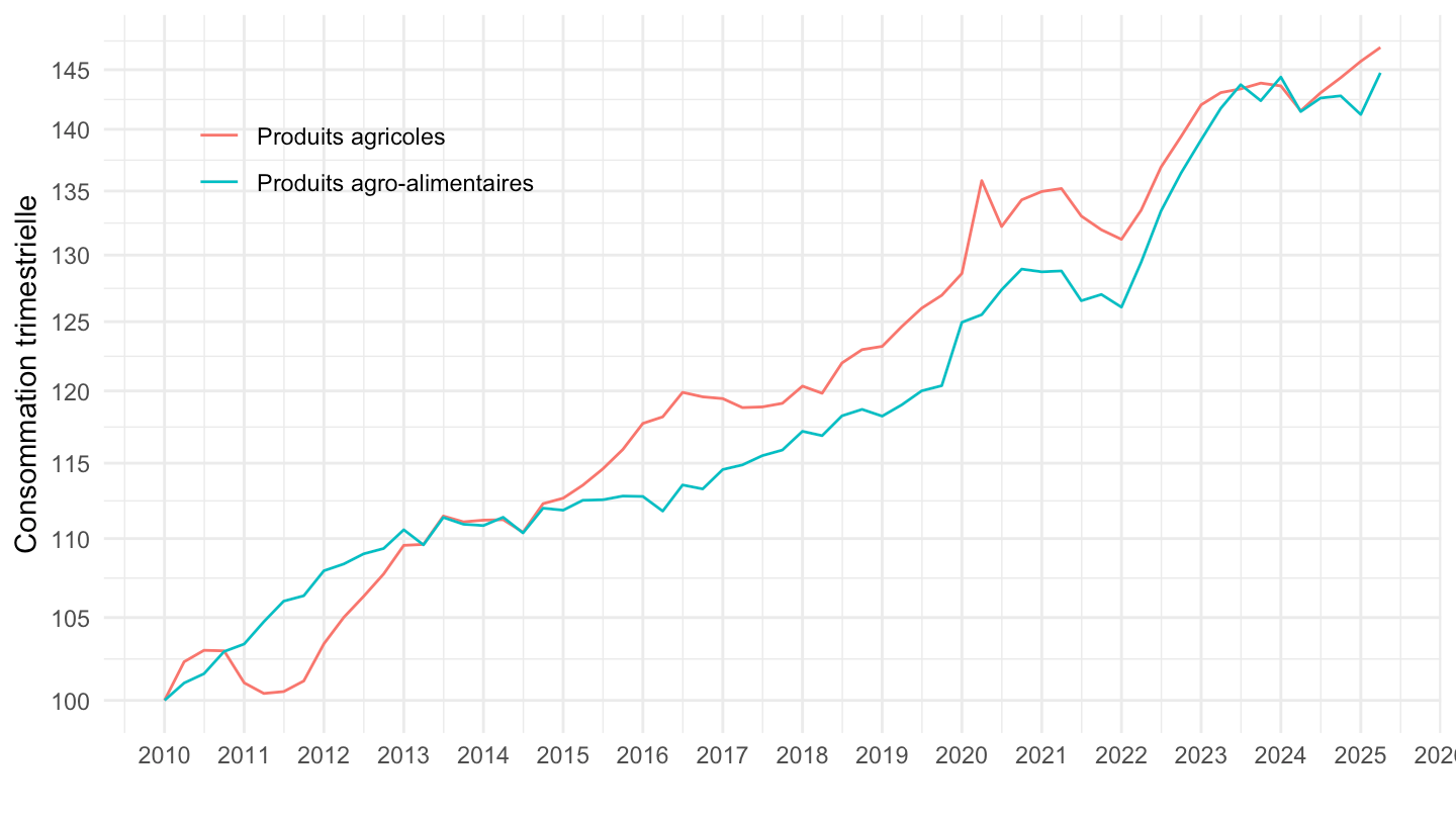
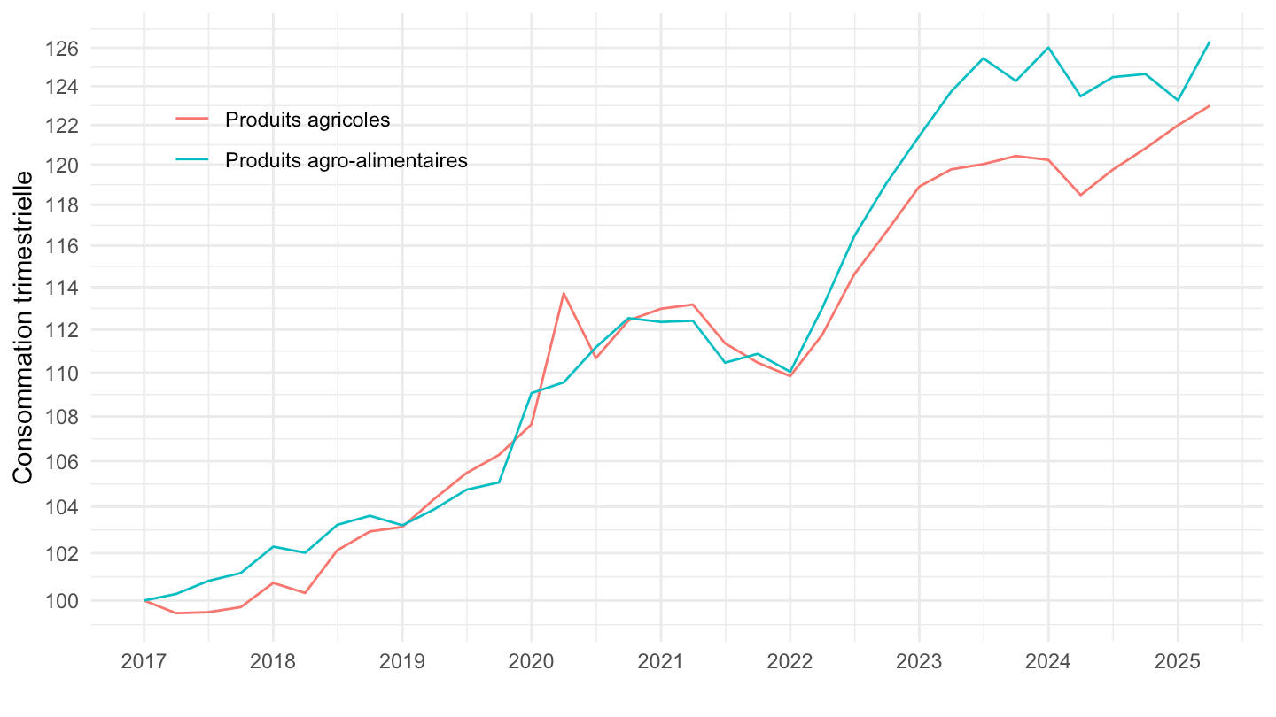
2017-
Code
t_conso_val %>%
  filter(variable %in% c("AZ", "C1"),
         date >= as.Date("2017-01-01")) %>%
  group_by(variable) %>%
  arrange(date) %>%
  mutate(value = 100*value/value[1]) %>%
  left_join(variable, by = "variable") %>%
  ggplot + geom_line(aes(x = date, y = value, color = Variable)) +
  theme_minimal() + ylab("Consommation trimestrielle") + xlab("") +
  theme(legend.title = element_blank(),
        legend.position = c(0.2, 0.8)) +
  scale_x_date(breaks = seq(1950, 2100, 1) %>% paste0("-01-01") %>% as.Date,
               labels = date_format("%Y")) +
  scale_y_log10(breaks = seq(70, 1000, 2))