Unemployment rate - annual data - tipsun20
Data - Eurostat
Info
Data on employment
| source | dataset | Title | .html | .rData |
|---|---|---|---|---|
| bls | jt | NA | NA | NA |
| bls | la | NA | NA | NA |
| bls | ln | NA | NA | NA |
| eurostat | nama_10_a10_e | Employment by A*10 industry breakdowns | 2026-06-04 | 2026-04-26 |
| eurostat | nama_10_a64_e | National accounts employment data by industry (up to NACE A*64) | 2026-06-04 | 2026-04-26 |
| eurostat | namq_10_a10_e | Employment A*10 industry breakdowns | 2025-05-24 | 2026-04-26 |
| eurostat | une_rt_m | Unemployment by sex and age – monthly data | 2026-06-04 | 2026-04-26 |
| oecd | ALFS_EMP | Employment by activities and status (ALFS) | 2024-04-16 | 2025-05-24 |
| oecd | EPL_T | Strictness of employment protection – temporary contracts | 2026-06-04 | 2023-12-10 |
| oecd | LFS_SEXAGE_I_R | LFS by sex and age - indicators | 2026-06-04 | 2024-04-15 |
| oecd | STLABOUR | Short-Term Labour Market Statistics | 2026-06-04 | 2025-01-17 |
DOWNLOAD_TIME
Code
tibble(DOWNLOAD_TIME = as.Date(file.info("~/iCloud/website/data/eurostat/tipsun20.RData")$mtime)) %>%
print_table_conditional()| DOWNLOAD_TIME |
|---|
| 2026-04-14 |
Last
Code
tipsun20 %>%
  group_by(time) %>%
  summarise(Nobs = n()) %>%
  arrange(desc(time)) %>%
  head(1) %>%
print_table_conditional()| time | Nobs |
|---|---|
| 2025 | 90 |
geo
Code
tipsun20 %>%
  left_join(geo, by = "geo") %>%
  group_by(geo, Geo) %>%
  summarise(Nobs = n()) %>%
  arrange(-Nobs) %>%
  mutate(Geo = ifelse(geo == "DE", "Germany", Geo)) %>%
  mutate(Flag = gsub(" ", "-", str_to_lower(Geo)),
         Flag = paste0('<img src="../../bib/flags/vsmall/', Flag, '.png" alt="Flag">')) %>%
  select(Flag, everything()) %>%
  {if (is_html_output()) datatable(., filter = 'top', rownames = F, escape = F) else .}
age
Code
tipsun20 %>%
  left_join(age, by = "age") %>%
  group_by(age, Age) %>%
  summarise(Nobs = n()) %>%
  arrange(-Nobs) %>%
print_table_conditional()| age | Age | Nobs |
|---|---|---|
| Y15-24 | From 15 to 24 years | 520 |
| Y15-74 | From 15 to 74 years | 520 |
| Y25-74 | From 25 to 74 years | 520 |
France, Germany, Italy, Spain, Portugal
Code
tipsun20 %>%
  filter(geo %in% c("FR", "DE", "PT", "ES", "IT"),
         age == "Y25-74") %>%
  year_to_date %>%
  left_join(geo, by = "geo") %>%
  left_join(colors, by = c("Geo" = "country")) %>%
  mutate(values = values/100) %>%
  ggplot + geom_line(aes(x = date, y = values, color = color)) + theme_minimal() +
  scale_color_identity() + add_5flags +
  scale_x_date(breaks = as.Date(paste0(seq(1960, 2100, 2), "-01-01")),
               labels = date_format("%Y")) +
  xlab("") + ylab("Unemployment, Percentage of active population") +
  scale_y_continuous(breaks = 0.01*seq(0, 200, 1),
                     labels = scales::percent_format(accuracy = 1))
France, Germany, Portugal
Code
tipsun20 %>%
  filter(geo %in% c("FR", "DE", "PT"),
         age == "Y25-74") %>%
  year_to_date %>%
  left_join(geo, by = "geo") %>%
  left_join(colors, by = c("Geo" = "country")) %>%
  mutate(values = values/100) %>%
  ggplot + geom_line(aes(x = date, y = values, color = color)) + theme_minimal() +
  scale_color_identity() + add_3flags +
  scale_x_date(breaks = as.Date(paste0(seq(1960, 2100, 2), "-01-01")),
               labels = date_format("%Y")) +
  xlab("") + ylab("Unemployment, Percentage of active population") +
  scale_y_continuous(breaks = 0.01*seq(0, 200, 1),
                     labels = scales::percent_format(accuracy = 1))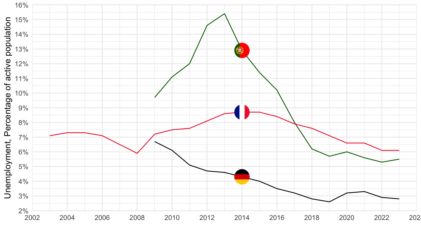
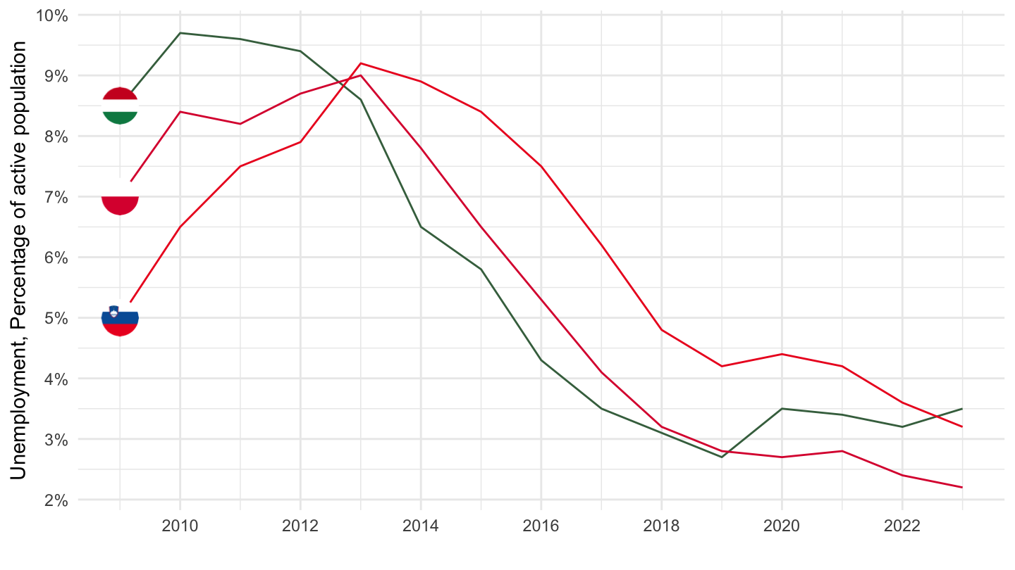
Poland, Hungary, Slovenia
Code
tipsun20 %>%
  filter(geo %in% c("PL", "HU", "SI"),
         age == "Y25-74") %>%
  year_to_date %>%
  left_join(geo, by = "geo") %>%
  left_join(colors, by = c("Geo" = "country")) %>%
  mutate(values = values/100) %>%
  ggplot + geom_line(aes(x = date, y = values, color = color)) + theme_minimal() +
  scale_color_identity() + add_3flags +
  scale_x_date(breaks = as.Date(paste0(seq(1960, 2100, 2), "-01-01")),
               labels = date_format("%Y")) +
  xlab("") + ylab("Unemployment, Percentage of active population") +
  scale_y_continuous(breaks = 0.01*seq(0, 200, 1),
                     labels = scales::percent_format(accuracy = 1))