Fred’s API

Data - Fred

Author

Info

source	dataset	.html	.RData
fred	api	2025-08-24	NA

LAST_COMPILE

LAST_COMPILE
2025-08-24

Info

API Documentation: https://data.oecd.org/api/sdmx-ml-documentation/
Example 1: https://stats.oecd.org/restsdmx/sdmx.ashx/GetData/GOV_DEBT/FIN+BEL.AMT.A.USD.3.
Example 2: https://stats.oecd.org/restsdmx/sdmx.ashx/GetData/QNA/AUS+AUT.GDP+B1_GE.CUR+VOBARSA.Q/all?startTime=2009-Q2&endTime=2011-Q4

Example 1

Code

"https://api.stlouisfed.org/fred/series?series_id=GNPCA&api_key=abcdefghijklmnopqrstuvwxyz123456"

# [1] "https://api.stlouisfed.org/fred/series?series_id=GNPCA&api_key=abcdefghijklmnopqrstuvwxyz123456"

Find a Data series, or multiple

Code

fredr_series_search_text(search_text = "cpi cbsa rent",
                         order_by = "popularity",
                         sort_order = "desc") %>%
  select(id, title) %>%
  {if (is_html_output()) datatable(., filter = 'top', rownames = F) else .}

API

(ref:oil) Oil Prices

Code

map_dfr(c("CPIAUCSL", "WTISPLC"), fredr) %>% 
  spread(series_id, value) %>%
  na.omit %>%
  mutate(WTISPLC_real = CPIAUCSL[860]* WTISPLC / CPIAUCSL) %>% 
  select(date, WTISPLC, WTISPLC.real = WTISPLC_real) %>% 
  gather(variable, value, -date) %>%
  mutate(variable_desc = case_when(variable == "WTISPLC" ~ "Oil Prices (WTI)",
                                   variable == "WTISPLC.real" ~ "Real Oil Prices (WTI)")) %>%
  select(variable, variable_desc, everything()) %>%
  ggplot(data = .) + 
  geom_line(aes(x = date, y = value, linetype = variable_desc, color = variable_desc)) +
  labs(x = "Observation Date", y = "Rate") + theme_minimal() +
  scale_color_manual(values = viridis(3)[1:2]) +
  geom_rect(data = nber_recessions %>%
              filter(Peak > as.Date("1928-01-01")), 
            aes(xmin = Peak, xmax = Trough, ymin = -Inf, ymax = +Inf), 
            fill = 'grey', alpha = 0.5) +
  theme(legend.title = element_blank(),
        legend.position = c(0.2, 0.8)) +
  scale_y_continuous(breaks = seq(0, 150, 25),
                labels = scales::dollar_format(accuracy = 1)) + 
  scale_x_date(breaks = as.Date(paste0(seq(1945, 2100, 5), "-01-01")),
               labels = date_format("%y"),
               limits = c(as.Date("1945-01-01"), as.Date("2020-01-01"))) +
  xlab("") + ylab("Oil Prices")

Modern Data

Code

fredr(series_id = "UNRATE") %>%
  tail(10) %>%
  {if (is_html_output()) print_table(.) else .}

date	series_id	value	realtime_start	realtime_end
2024-10-01	UNRATE	4.1	2025-08-21	2025-08-21
2024-11-01	UNRATE	4.2	2025-08-21	2025-08-21
2024-12-01	UNRATE	4.1	2025-08-21	2025-08-21
2025-01-01	UNRATE	4.0	2025-08-21	2025-08-21
2025-02-01	UNRATE	4.1	2025-08-21	2025-08-21
2025-03-01	UNRATE	4.2	2025-08-21	2025-08-21
2025-04-01	UNRATE	4.2	2025-08-21	2025-08-21
2025-05-01	UNRATE	4.2	2025-08-21	2025-08-21
2025-06-01	UNRATE	4.1	2025-08-21	2025-08-21
2025-07-01	UNRATE	4.2	2025-08-21	2025-08-21

Code

fredr(series_id = "UNRATE",
      observation_start = as.Date("1990-01-01")) %>%
  head(10) %>%
  {if (is_html_output()) print_table(.) else .}

date	series_id	value	realtime_start	realtime_end
1990-01-01	UNRATE	5.4	2025-08-21	2025-08-21
1990-02-01	UNRATE	5.3	2025-08-21	2025-08-21
1990-03-01	UNRATE	5.2	2025-08-21	2025-08-21
1990-04-01	UNRATE	5.4	2025-08-21	2025-08-21
1990-05-01	UNRATE	5.4	2025-08-21	2025-08-21
1990-06-01	UNRATE	5.2	2025-08-21	2025-08-21
1990-07-01	UNRATE	5.5	2025-08-21	2025-08-21
1990-08-01	UNRATE	5.7	2025-08-21	2025-08-21
1990-09-01	UNRATE	5.9	2025-08-21	2025-08-21
1990-10-01	UNRATE	5.9	2025-08-21	2025-08-21

What are other data series for unemployment?

Code

unemp.1929.1942 <- fredr(series_id = "M0892AUSM156SNBR")
unemp.1947.1966 <- fredr(series_id = "M0892CUSM156NNBR")
unemp.1948.now <- fredr(series_id = "UNRATE")

unemp.1929.1942 %>%
  head %>%
  {if (is_html_output()) print_table(.) else .}

date	series_id	value	realtime_start	realtime_end
1929-04-01	M0892AUSM156SNBR	0.69	2025-08-24	2025-08-24
1929-05-01	M0892AUSM156SNBR	1.65	2025-08-24	2025-08-24
1929-06-01	M0892AUSM156SNBR	2.06	2025-08-24	2025-08-24
1929-07-01	M0892AUSM156SNBR	0.79	2025-08-24	2025-08-24
1929-08-01	M0892AUSM156SNBR	0.04	2025-08-24	2025-08-24
1929-09-01	M0892AUSM156SNBR	0.91	2025-08-24	2025-08-24

Code

fredr_series_search_text(search_text = "unemployment",
                         order_by = "popularity",
                         sort_order = "desc") %>%
  select(id, observation_start, title) %>%
  as.tibble %>%
  head(20) %>%
  {if (is_html_output()) print_table(.) else .}

id	observation_start	title
CPIAUCSL	1947-01-01	Consumer Price Index for All Urban Consumers: All Items in U.S. City Average
UNRATE	1948-01-01	Unemployment Rate
SAHMREALTIME	1959-12-01	Real-time Sahm Rule Recession Indicator
PAYEMS	1939-01-01	All Employees, Total Nonfarm
ICSA	1967-01-07	Initial Claims
CCSA	1967-01-07	Continued Claims (Insured Unemployment)
CES0500000003	2006-03-01	Average Hourly Earnings of All Employees, Total Private
UNEMPLOY	1948-01-01	Unemployment Level
U6RATE	1994-01-01	Total Unemployed, Plus All Persons Marginally Attached to the Labor Force, Plus Total Employed Part Time for Economic Reasons, as a Percent of the Civilian Labor Force Plus All Persons Marginally Attached to the Labor Force (U-6)
NROU	1949-01-01	Noncyclical Rate of Unemployment
LNS14000006	1972-01-01	Unemployment Rate - Black or African American
IC4WSA	1967-01-28	4-Week Moving Average of Initial Claims
SAHMCURRENT	1949-03-01	Sahm Rule Recession Indicator
ICNSA	1967-01-07	Initial Claims
WEI	2008-01-05	Weekly Economic Index (Lewis-Mertens-Stock)
USSLIND	1982-01-01	Leading Index for the United States
CAUR	1976-01-01	Unemployment Rate in California
LNS14000024	1948-01-01	Unemployment Rate - 20 Yrs. & over
CC4WSA	1967-01-28	4-Week Moving Average of Continued Claims (Insured Unemployment)
USPHCI	1979-01-01	Coincident Economic Activity Index for the United States

Code

fredr_series_search_text(search_text = "price index",
                         order_by = "popularity",
                         sort_order = "desc") %>%
  select(id, title) %>%
  as.tibble %>%
  head(20) %>%
  {if (is_html_output()) print_table(.) else .}

id	title
CPIAUCSL	Consumer Price Index for All Urban Consumers: All Items in U.S. City Average
SP500	S&P 500
APU0000708111	Average Price: Eggs, Grade A, Large (Cost per Dozen) in U.S. City Average
CSUSHPINSA	S&P CoreLogic Case-Shiller U.S. National Home Price Index
FPCPITOTLZGUSA	Inflation, consumer prices for the United States
DFII10	Market Yield on U.S. Treasury Securities at 10-Year Constant Maturity, Quoted on an Investment Basis, Inflation-Indexed
CPILFESL	Consumer Price Index for All Urban Consumers: All Items Less Food and Energy in U.S. City Average
VIXCLS	CBOE Volatility Index: VIX
PCEPI	Personal Consumption Expenditures: Chain-type Price Index
CORESTICKM159SFRBATL	Sticky Price Consumer Price Index less Food and Energy
APU0000703112	Average Price: Ground Beef, 100% Beef (Cost per Pound/453.6 Grams) in U.S. City Average
CPIAUCNS	Consumer Price Index for All Urban Consumers: All Items in U.S. City Average
PPIACO	Producer Price Index by Commodity: All Commodities
PCEPILFE	Personal Consumption Expenditures Excluding Food and Energy (Chain-Type Price Index)
CSUSHPISA	S&P CoreLogic Case-Shiller U.S. National Home Price Index
APU000072610	Average Price: Electricity per Kilowatt-Hour in U.S. City Average
CUSR0000SETA02	Consumer Price Index for All Urban Consumers: Used Cars and Trucks in U.S. City Average
USSTHPI	All-Transactions House Price Index for the United States
CPALTT01USM657N	Consumer Price Index: All Items: Total for United States
APU0000709112	Average Price: Milk, Fresh, Whole, Fortified (Cost per Gallon/3.8 Liters) in U.S. City Average

Integrate with tidyverse package

Code

fredr_series_search_text(search_text = "federal funds",
                         order_by = "popularity",
                         sort_order = "desc",
                         limit = 1) %>%
  pull(id) %>%
  map_dfr(., fredr) %>%
  filter(date >= as.Date("1990-01-01")) %>%
  ggplot(.) + 
  geom_line(aes(x = date, y = value/100)) +
  labs(x = "Observation Date", y = "Rate") + theme_minimal() +
  theme(legend.title = element_blank(),
        legend.position = c(0.4, 0.8)) +
  scale_x_date(breaks = as.Date(paste0(seq(1990, 2100, 2), "-01-01")),
               labels = date_format("%y")) +
  scale_y_continuous(breaks = seq(-0.01, 0.12, 0.01),
                     labels = scales::percent_format(accuracy = 1)) + 
  xlab("") + ylab("10-Year Treasury Rate")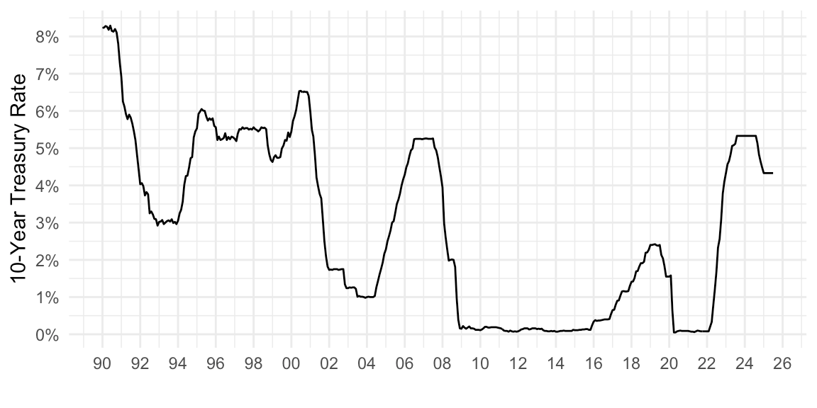

Look for series: debt and gross domestic product

Code

fredr_series_search_text(search_text = "debt",
                         order_by = "popularity",
                         sort_order = "desc",
                         limit = 5) %>%
  as.tibble %>%
  arrange(observation_start) %>%
  select(id, title) %>%
  {if (is_html_output()) print_table(.) else .}

id	title
GFDEBTN	Federal Debt: Total Public Debt
GFDEGDQ188S	Federal Debt: Total Public Debt as Percent of Gross Domestic Product
WTREGEN	Liabilities and Capital: Liabilities: Deposits with F.R. Banks, Other Than Reserve Balances: U.S. Treasury, General Account: Week Average
BAMLH0A0HYM2	ICE BofA US High Yield Index Option-Adjusted Spread
RRPONTSYD	Overnight Reverse Repurchase Agreements: Treasury Securities Sold by the Federal Reserve in the Temporary Open Market Operations

Code

fredr_series_search_text(search_text = "gross domestic product",
                         order_by = "popularity",
                         sort_order = "desc",
                         limit = 5) %>%
  as.tibble %>%
  arrange(observation_start) %>%
  select(id, title) %>%
  {if (is_html_output()) print_table(.) else .}

id	title
FYFSGDA188S	Federal Surplus or Deficit [-] as Percent of Gross Domestic Product
PAYEMS	All Employees, Total Nonfarm
GDP	Gross Domestic Product
GDPC1	Real Gross Domestic Product
GFDEGDQ188S	Federal Debt: Total Public Debt as Percent of Gross Domestic Product

Code

fredr_series_observations(series_id = "UNRATE",
                          observation_start = as.Date("2018-01-01"),
                          frequency = "q",
                          units = "chg") %>%
  {if (is_html_output()) print_table(.) else .}

date	series_id	value	realtime_start	realtime_end
2018-01-01	UNRATE	-0.1333333	2025-08-24	2025-08-24
2018-04-01	UNRATE	-0.1000000	2025-08-24	2025-08-24
2018-07-01	UNRATE	-0.1666667	2025-08-24	2025-08-24
2018-10-01	UNRATE	0.0666667	2025-08-24	2025-08-24
2019-01-01	UNRATE	0.0333333	2025-08-24	2025-08-24
2019-04-01	UNRATE	-0.2333333	2025-08-24	2025-08-24
2019-07-01	UNRATE	-0.0333333	2025-08-24	2025-08-24
2019-10-01	UNRATE	0.0000000	2025-08-24	2025-08-24
2020-01-01	UNRATE	0.2333333	2025-08-24	2025-08-24
2020-04-01	UNRATE	9.1666667	2025-08-24	2025-08-24
2020-07-01	UNRATE	-4.2000000	2025-08-24	2025-08-24
2020-10-01	UNRATE	-2.0333333	2025-08-24	2025-08-24
2021-01-01	UNRATE	-0.5333333	2025-08-24	2025-08-24
2021-04-01	UNRATE	-0.3000000	2025-08-24	2025-08-24
2021-07-01	UNRATE	-0.8666667	2025-08-24	2025-08-24
2021-10-01	UNRATE	-0.8666667	2025-08-24	2025-08-24
2022-01-01	UNRATE	-0.3666667	2025-08-24	2025-08-24
2022-04-01	UNRATE	-0.2000000	2025-08-24	2025-08-24
2022-07-01	UNRATE	-0.1000000	2025-08-24	2025-08-24
2022-10-01	UNRATE	0.0333333	2025-08-24	2025-08-24
2023-01-01	UNRATE	-0.0333333	2025-08-24	2025-08-24
2023-04-01	UNRATE	0.0000000	2025-08-24	2025-08-24
2023-07-01	UNRATE	0.1333333	2025-08-24	2025-08-24
2023-10-01	UNRATE	0.1333333	2025-08-24	2025-08-24
2024-01-01	UNRATE	0.0333333	2025-08-24	2025-08-24
2024-04-01	UNRATE	0.1666667	2025-08-24	2025-08-24
2024-07-01	UNRATE	0.1666667	2025-08-24	2025-08-24
2024-10-01	UNRATE	-0.0333333	2025-08-24	2025-08-24
2025-01-01	UNRATE	-0.0333333	2025-08-24	2025-08-24
2025-04-01	UNRATE	0.0666667	2025-08-24	2025-08-24
2025-07-01	UNRATE	NA	2025-08-24	2025-08-24

Integrate the purrr package

This is how to create a wide database with various FRED Databases:

Code

map_dfr(c("FEDFUNDS", "UNRATE"), fredr) %>%
  spread(series_id, value) %>%
  top_n(10) %>%
  {if (is_html_output()) print_table(.) else .}

date	realtime_start	realtime_end	FEDFUNDS	UNRATE
1982-10-01	2025-08-21	2025-08-21	9.71	10.4
1982-11-01	2025-08-21	2025-08-21	9.20	10.8
1982-12-01	2025-08-21	2025-08-21	8.95	10.8
1983-01-01	2025-08-21	2025-08-21	8.68	10.4
1983-02-01	2025-08-21	2025-08-21	8.51	10.4
1983-03-01	2025-08-21	2025-08-21	8.77	10.3
1983-04-01	2025-08-21	2025-08-21	8.80	10.2
2020-04-01	2025-08-21	2025-08-21	0.05	14.8
2020-05-01	2025-08-21	2025-08-21	0.05	13.2
2020-06-01	2025-08-21	2025-08-21	0.08	11.0
2020-07-01	2025-08-21	2025-08-21	0.09	10.2

This is how to map them:

Code

map_dfr(c("UNRATE", "FEDFUNDS"), fredr) %>%
  ggplot(.) + theme_minimal() + 
  geom_line(aes(x = date, y = value/100, color = series_id)) +
  labs(x = "Observation Date", y = "Rate", linetype = "Series") +
  scale_color_manual(values = viridis(3)[1:2]) +
  theme(legend.title = element_blank(),
        legend.position = c(0.3, 0.8)) +
  scale_x_date(breaks = as.Date(paste0(seq(1920, 2100, 5), "-01-01")),
               labels = date_format("%y")) +
  scale_y_continuous(breaks = seq(-0.01, 0.3, 0.02),
                     labels = scales::percent_format(accuracy = 1)) + 
  xlab("") + ylab("") + theme(legend.title = element_blank())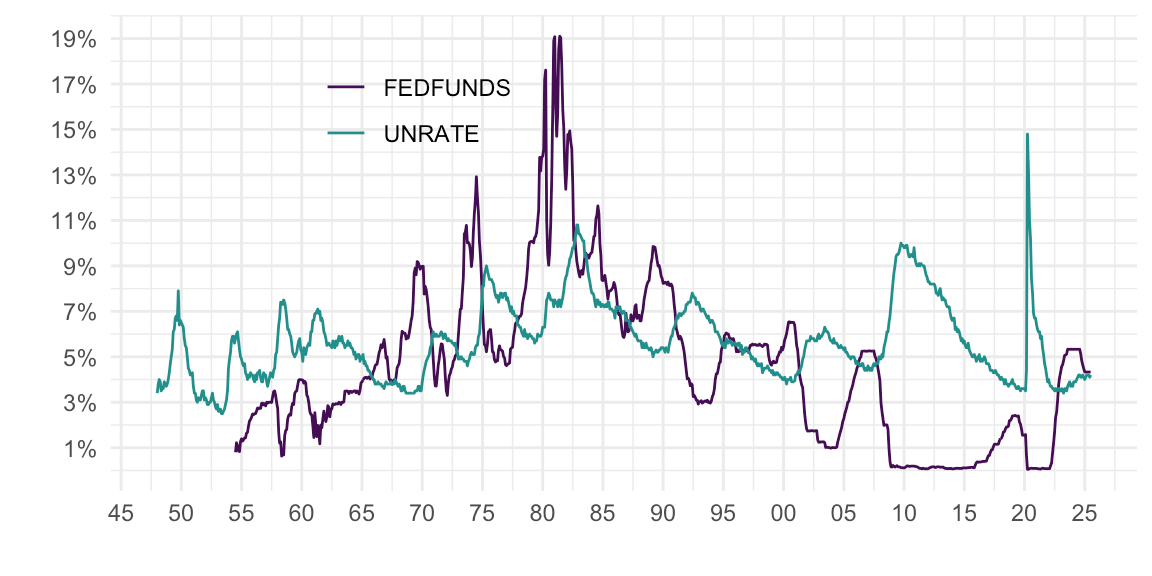

Code

params <- list(series_id = c("UNRATE", "OILPRICE"),
               frequency = c("m", "q"))

pmap_dfr(.l = params,
         .f = ~ fredr(series_id = .x, frequency = .y)) %>%
  head(10) %>%
  {if (is_html_output()) print_table(.) else .}

date	series_id	value	realtime_start	realtime_end
1948-01-01	UNRATE	3.4	2025-08-21	2025-08-21
1948-02-01	UNRATE	3.8	2025-08-21	2025-08-21
1948-03-01	UNRATE	4.0	2025-08-21	2025-08-21
1948-04-01	UNRATE	3.9	2025-08-21	2025-08-21
1948-05-01	UNRATE	3.5	2025-08-21	2025-08-21
1948-06-01	UNRATE	3.6	2025-08-21	2025-08-21
1948-07-01	UNRATE	3.6	2025-08-21	2025-08-21
1948-08-01	UNRATE	3.9	2025-08-21	2025-08-21
1948-09-01	UNRATE	3.8	2025-08-21	2025-08-21
1948-10-01	UNRATE	3.7	2025-08-21	2025-08-21

Household Debt Service Payments as a Percent of Disposable Income

Code

map_dfr(c("TDSP"), fredr) %>%
  ggplot(data = ., mapping = aes(x = date, y = value/100)) +
  geom_line() + theme_minimal() +
  labs(x = "Observation Date", y = "Rate", color = "Series") +
  theme(legend.title = element_blank(),
        legend.position = c(0.4, 0.8)) +
  scale_x_date(breaks = as.Date(paste0(seq(1970, 2100, 5), "-01-01")),
               labels = date_format("%y")) +
  scale_y_continuous(breaks = seq(-0.01, 0.30, 0.01),
                     labels = scales::percent_format(accuracy = 1)) + 
  xlab("") + ylab("") + theme(legend.title = element_blank())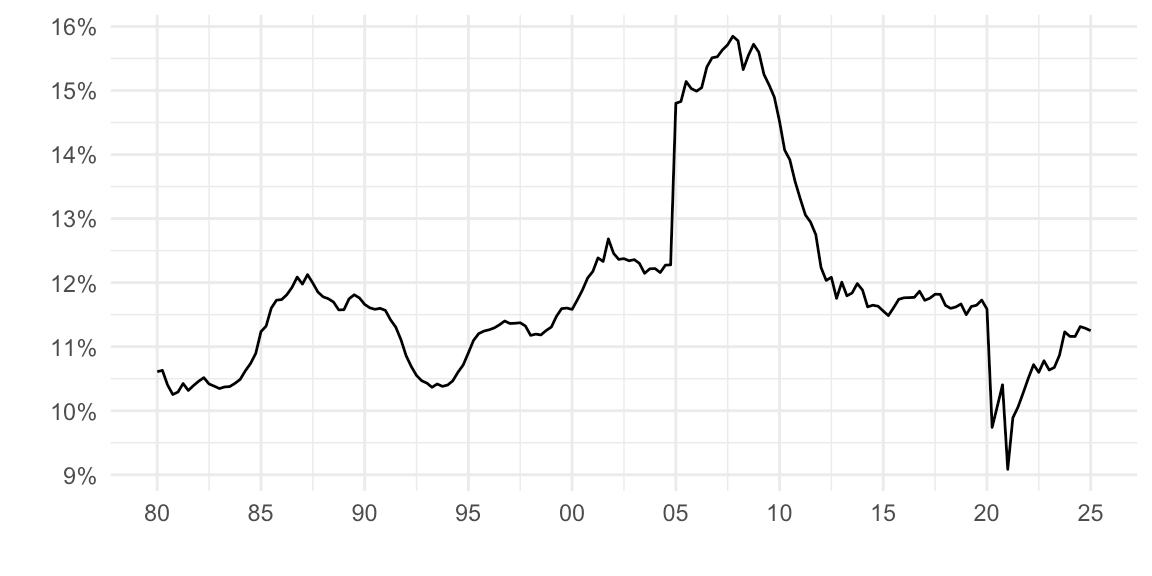

Nominal and Real Oil Prices

Oil Prices and Price Index

Data from FRED - Federal Reserve Bank of St. Louis:

CPIAUCSL: Consumer Price Index for All Urban Consumers: All Items. Available at: https://fred.stlouisfed.org/series/CPIAUCSL
WTISPLC: Spot Crude Oil Price: West Texas Intermediate (WTI). Available at: https://fred.stlouisfed.org/series/WTISPLC

Code

map_dfr(c("CPIAUCSL", "WTISPLC"), fredr) %>%
  ggplot(data = ., mapping = aes(x = date, y = value, linetype = series_id)) +
  geom_line() +
  labs(x = "Observation Date", y = "Rate", color = "Series") +
  theme_minimal() + xlab("") + ylab("") + theme(legend.title = element_blank())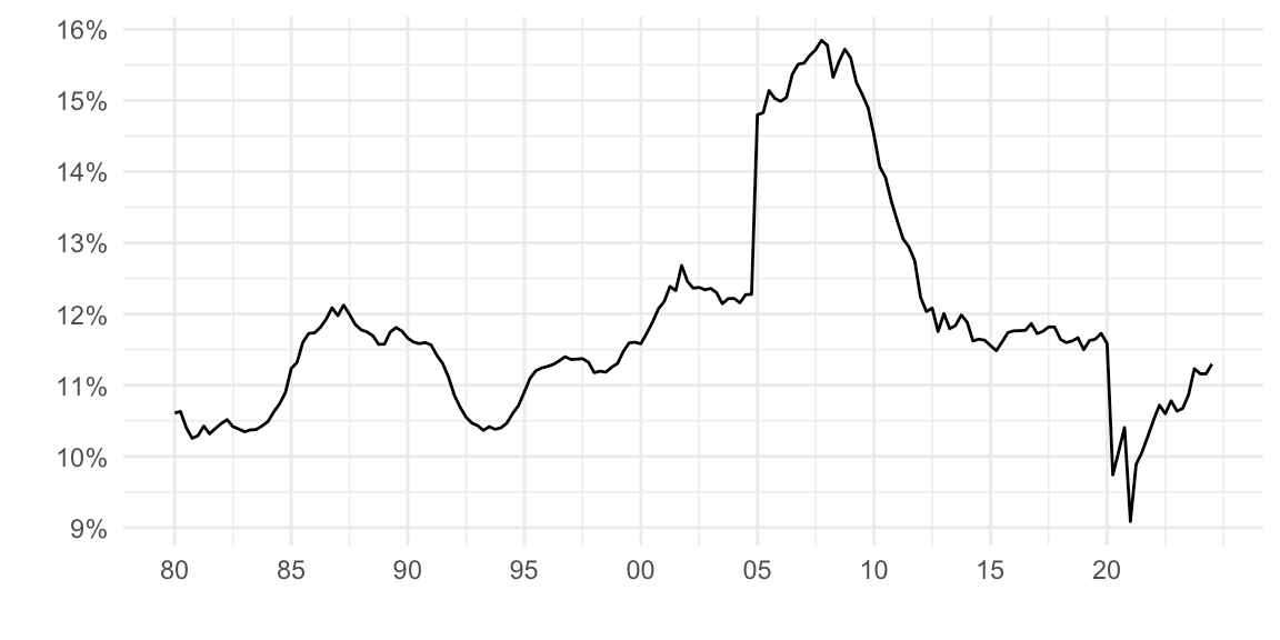

Real Oil Prices

Code

map_dfr(c("CPIAUCSL", "WTISPLC"), fredr) %>%
  spread(series_id, value) %>%
  # Current House Prices from August 2018
  na.omit %>%
  mutate(WTISPLC_real = CPIAUCSL[860]* WTISPLC / CPIAUCSL) %>%
  select(-CPIAUCSL) %>%
  gather(series_id, value, -date) %>%
  ggplot(data = ., mapping = aes(x = date, y = value, linetype = series_id)) +
  geom_line() + labs(x = "Observation Date", y = "Rate", color = "Series") +
  theme_minimal() + xlab("") + ylab("") + theme(legend.title = element_blank())

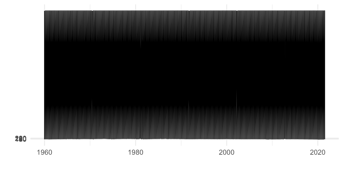
Passenger car registration

Code

fredr_series_search_text(search_text = "Passenger Car Registrations",
                         order_by = "popularity",
                         sort_order = "desc",
                         limit = 5) %>%
  as.tibble %>%
  select(observation_start, id, title, everything()) %>%
  arrange(observation_start) %>%
  select(2, 3, frequency) %>%
  {if (is_html_output()) print_table(.) else .}

id	title	frequency
A01108USA258NNBR	Automobile Registrations, Passenger Cars, Total for United States	Annual, End of Year
M01109USM543NNBR	New Passenger Car Registrations for United States	Monthly
USASACRMISMEI	Production, Sales, Work Started and Orders: Passenger Car Registrations: Economic Activity: Wholesale and Retail Trade and Repair of Motor Vehicles and Motorcycles for United States	Monthly
USASLRTCR03MLSAM	Sales: Retail Trade: Car Registration: Passenger Cars for United States	Monthly
USASACRQISMEI	Sales: Retail Trade: Car Registration: Passenger Cars for United States	Quarterly

Code

map_dfr(c("USASACRQISMEI"), fredr) %>%
  spread(series_id, value) %>%
  na.omit %>%
  # Current House Prices from August 2018
  gather(series_id, value, -date) %>%
  ggplot(data = ., mapping = aes(x = date, y = value)) +
  geom_line() + 
  scale_y_continuous(breaks = seq(80, 220, 20)) + xlab("") + ylab("") +
  theme_minimal() + theme(legend.title = element_blank())