European Central Bank’s API

Data - ecb

Author

Info

List of APIs

source	dataset	Title	.html	.rData
bdf	api	NA	NA	NA
bea	api	NA	NA	NA
bis	api	NA	NA	NA
bls	api	NA	NA	NA
dbnomics	api	NA	NA	NA
ecb	api	NA	NA	NA
eurostat	api	NA	NA	NA
imf	api	NA	NA	NA
insee	api	NA	NA	NA
oecd	api	OECD's API	2024-05-07	2024-04-16
wdi	api	NA	NA	NA

LAST_COMPILE

LAST_COMPILE
2026-02-08

Data Structure Definition (DSD)

Code

new <- paste0(base_url, "codelist/all/all/latest?detail=allstubs") %>%
  readSDMX() %>%
  slot("codelists")


new2 <- paste0(base_url, "datastructure/ECB/ECB_EXR1/1.0?references=children") %>%
  readSDMX()

Info

Help for the SDMX protocol: https://sdw-wsrest.ecb.europa.eu/help/
Datasets from the ECB: https://www.ecb.europa.eu/stats/ecb_statistics/escb/html/index.en.html
Statistical Data Warehouse: http://sdw.ecb.europa.eu/browse.do?node=bbn2883

US Dollar / Euro Exchange Rate

Annual

Code

paste0(base_url, "data/EXR/M.USD.EUR.SP00.A") %>%
  readSDMX() %>%
  as_tibble %>%
  month_to_date() %>%
  ggplot(.) + geom_line(aes(x = date, y = obsValue)) + 
  theme_minimal() + xlab("") + ylab("") +
  scale_x_date(breaks = seq(1960, 2026, 2) %>% paste0("-01-01") %>% as.Date,
               labels = date_format("%Y")) +
  scale_y_continuous(breaks = seq(0, 10, 0.1),
                     labels = dollar_format(accuracy = 0.1, suffix = "/€")) +
  scale_color_manual(values = viridis(5)[1:4]) +
  theme(legend.position = c(0.8, 0.80),
        legend.title = element_blank())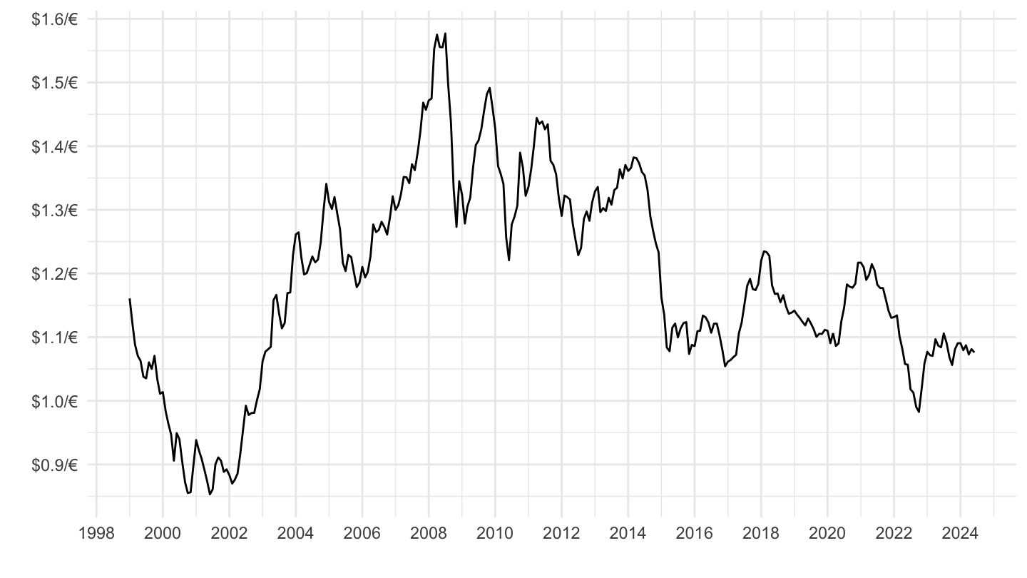

Quarterly

Code

paste0(base_url, "data/EXR/Q.USD.EUR.SP00.A") %>%
  readSDMX() %>%
  as_tibble %>%
  quarter_to_date() %>%
  ggplot(.) + geom_line(aes(x = date, y = obsValue)) + 
  theme_minimal() + xlab("") + ylab("") +
  scale_x_date(breaks = seq(1960, 2026, 2) %>% paste0("-01-01") %>% as.Date,
               labels = date_format("%Y")) +
  scale_y_continuous(breaks = seq(0, 10, 0.1),
                     labels = dollar_format(accuracy = 0.1, suffix = "/€")) +
  scale_color_manual(values = viridis(5)[1:4]) +
  theme(legend.position = c(0.8, 0.80),
        legend.title = element_blank())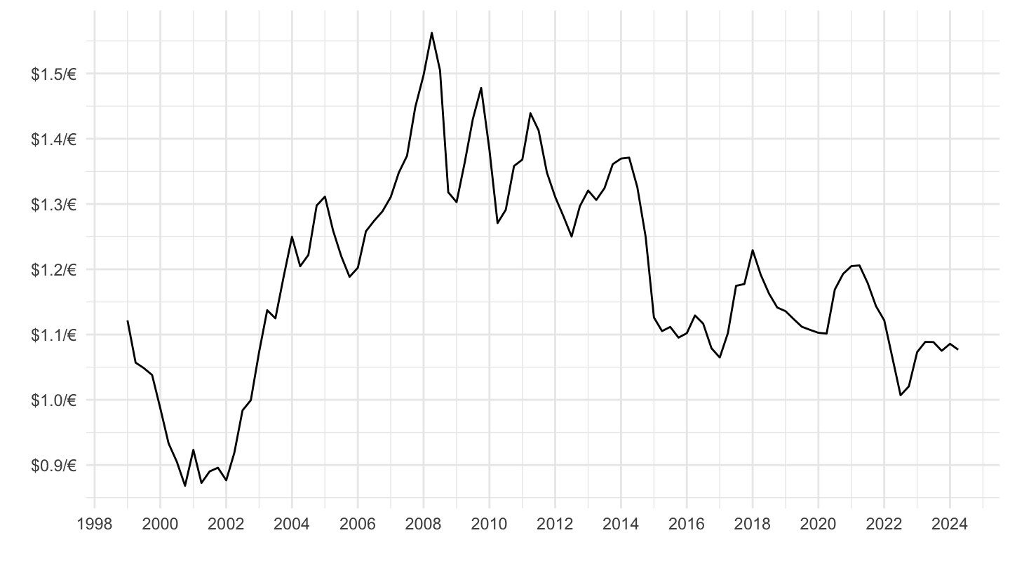

Financial Markets

Euribor 1-year

Source: https://sdw.ecb.europa.eu/quickview.do?SERIES_KEY=143.FM.M.U2.EUR.RT.MM.EURIBOR1YD_.HSTA

Code

paste0(base_url, "data/FM/M.U2.EUR.RT.MM.EURIBOR1YD_.HSTA") %>% readSDMX() %>% as_tibble %>%
  mutate(obsTime = zoo::as.yearmon(obsTime, format = "%Y-%m")) %>%
  ggplot + geom_line(aes(x = obsTime, y = obsValue/100)) +
  xlab("") + ylab("Euribor 1-year") + theme_minimal() +
  zoo::scale_x_yearmon(format = "%Y-%m") +
  theme(legend.position = c(0.65, 0.25),
        legend.title = element_blank()) +
  scale_y_continuous(breaks = 0.01*seq(-100, 90, 0.5),
                     labels = scales::percent_format(accuracy = .1)) +
  geom_hline(yintercept = 0, linetype = "dashed")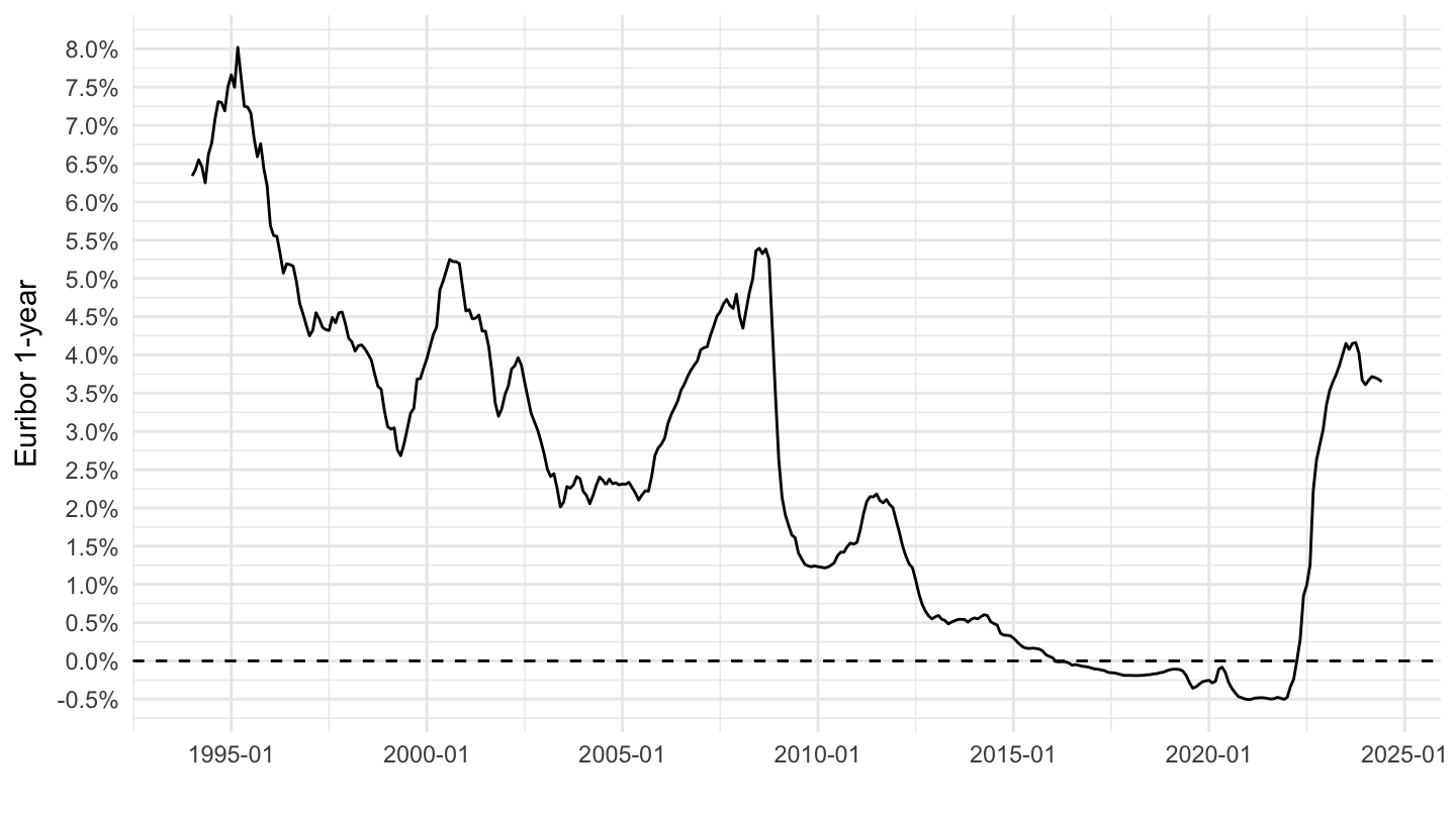

Interest rates

Interest rate on minimum reserves

Code

paste0(base_url, "data/BSI/M.U2.N.E.IRR.X.X.U2.0000.Z0Z.I") %>% readSDMX() %>% as_tibble %>%
  mutate(obsTime = zoo::as.yearmon(obsTime, format = "%Y-%m")) %>%
  ggplot + geom_line(aes(x = obsTime, y = obsValue/100)) +
  xlab("") + ylab("Interest rate on minimum reserves") + theme_minimal() +
  zoo::scale_x_yearmon(format = "%Y-%m") +
  theme(legend.position = c(0.65, 0.25),
        legend.title = element_blank()) +
  scale_y_continuous(breaks = 0.01*seq(-100, 90, 0.5),
                     labels = scales::percent_format(accuracy = .1)) +
  geom_hline(yintercept = 0, linetype = "dashed")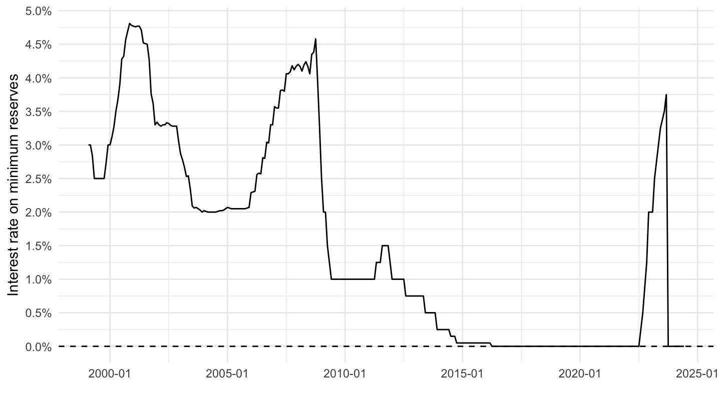

Reserves, required and excess, Current Account

Linear

Code

paste0(base_url, "data/BSI/M.U2.N.R.LRE.X.1.A1.3000.Z01.E") %>% readSDMX() %>% as_tibble %>%
  bind_rows(paste0(base_url, "data/BSI/M.U2.N.R.LRE.X.1.A1.3000.Z01.E") %>% readSDMX() %>% as_tibble) %>%
  bind_rows(paste0(base_url, "data/ILM/M.U2.C.L020100.U2.EUR") %>% readSDMX() %>% as_tibble) %>%
  rename(OBS_VALUE = obsValue) %>%
  month_to_date %>%
  mutate(OBS_VALUE = OBS_VALUE/1000) %>%
  ggplot + geom_line(aes(x = date, y = OBS_VALUE, color = TITLE)) +
  ylab("Required and Excess reserves") + xlab("") + theme_minimal() +
  theme(legend.position = c(0.45, 0.9),
        legend.title = element_blank()) +
  scale_y_continuous(breaks = seq(0, 10000, 500),
                labels = dollar_format(acc = 1, pre = "", su = "Bn€")) +
  scale_x_date(breaks = as.Date(paste0(seq(1940, 2100, 2), "-01-01")),
               labels = date_format("%Y"))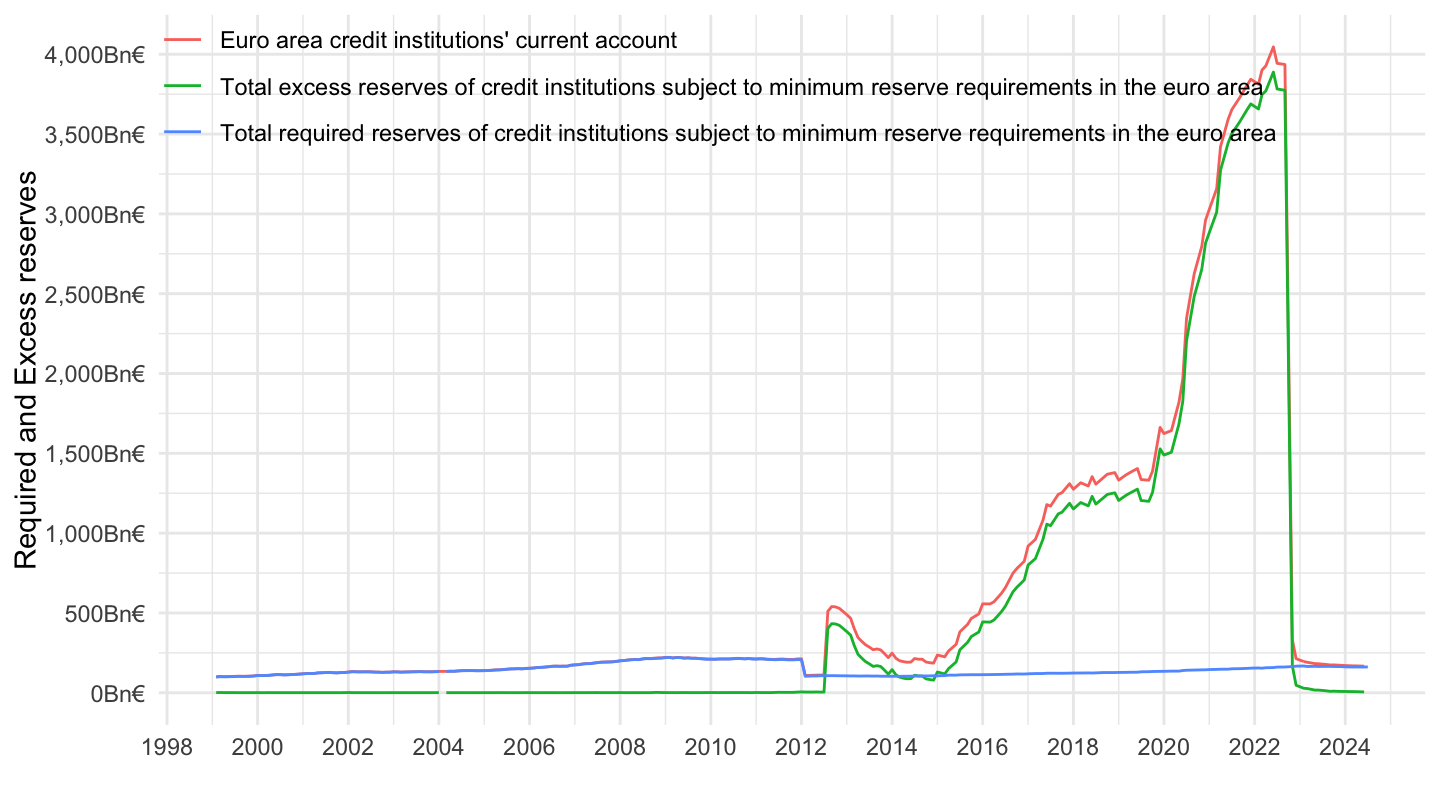

Log

Code

paste0(base_url, "data/BSI/M.U2.N.R.LRE.X.1.A1.3000.Z01.E") %>% readSDMX() %>% as_tibble %>%
  bind_rows(paste0(base_url, "data/BSI/M.U2.N.R.LRE.X.1.A1.3000.Z01.E") %>% readSDMX() %>% as_tibble) %>%
  bind_rows(paste0(base_url, "data/ILM/M.U2.C.L020100.U2.EUR") %>% readSDMX() %>% as_tibble) %>%
  rename(OBS_VALUE = obsValue) %>%
  month_to_date %>%
  mutate(OBS_VALUE = OBS_VALUE/1000) %>%
  ggplot + geom_line(aes(x = date, y = OBS_VALUE, color = TITLE)) +
  ylab("Required and Excess reserves") + xlab("") + theme_minimal() +
  theme(legend.position = c(0.45, 0.9),
        legend.title = element_blank()) +
  scale_y_log10(breaks = 10^(seq(0, 10, 1)),
                labels = dollar_format(acc = 1, pre = "", su = "Bn€")) +
  scale_x_date(breaks = as.Date(paste0(seq(1940, 2100, 2), "-01-01")),
               labels = date_format("%Y"))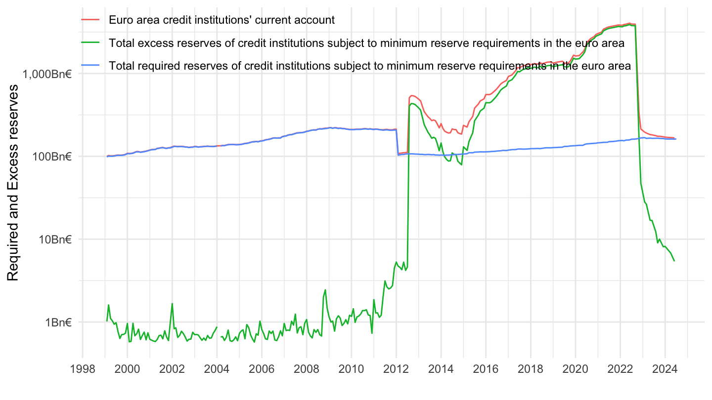

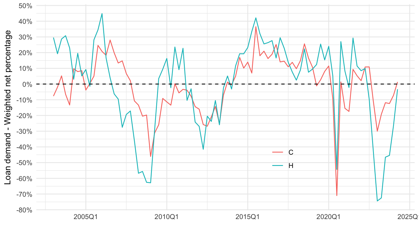
Bank Lending Statistics

Loan demand - Weighted net percentage

Code

paste0(base_url, "data/BLS/Q.U2.ALL.Z.H.H+C.B3.ZZ.D.WFNET") %>%
  readSDMX() %>%
  as_tibble %>%
  mutate(obsTime = zoo::as.yearqtr(obsTime, format = "%Y-Q%q")) %>%
  ggplot + geom_line(aes(x = obsTime, y = obsValue/100, color = BLS_COUNT_DETAIL)) +
  xlab("") + ylab("Loan demand - Weighted net percentage") + theme_minimal() +
  zoo::scale_x_yearqtr(format = "%YQ%q") +
  theme(legend.position = c(0.65, 0.25),
        legend.title = element_blank()) +
  scale_y_continuous(breaks = 0.01*seq(-100, 90, 10),
                     labels = scales::percent_format(accuracy = 1)) +
  geom_hline(yintercept = 0, linetype = "dashed")