Institut National de la Statistique et des Etudes Economiques’ API
Données - INSEE
Info
List of APIs
LAST_COMPILE
| LAST_COMPILE |
|---|
| 2026-07-26 |
List Datasets
Français
Code
"https://bdm.insee.fr/series/sdmx/dataflow" %>%
  readSDMX %>%
  as_tibble %>%
  select(id, Name.fr) %>%
  {if (is_html_output()) datatable(., filter = 'top', rownames = F) else .}
English
Code
"https://bdm.insee.fr/series/sdmx/dataflow" %>%
  readSDMX %>%
  as_tibble %>%
  select(id, Name.en) %>%
  {if (is_html_output()) datatable(., filter = 'top', rownames = F) else .}
Using IDBANKS
France, Paris, Lyon, Marseille
Code
"010567006+010567010+010567012+010567056" %>%
  paste0("https://www.bdm.insee.fr/series/sdmx/data/SERIES_BDM/", .) %>%
  readSDMX %>%
  as_tibble %>%
  quarter_to_date %>%
  mutate(OBS_VALUE = as.numeric(OBS_VALUE)) %>%
  mutate(TITLE_FR = gsub("Indice des prix des logements anciens - ", "", TITLE_FR),
         TITLE_FR = gsub(" - Appartements - Base 100 en moyenne annuelle 2015", "", TITLE_FR),
         TITLE_FR = gsub(" - Série brute", "", TITLE_FR)) %>%
  group_by(REF_AREA) %>%
  mutate(OBS_VALUE = 100*OBS_VALUE / OBS_VALUE[date == as.Date("1998-01-01")]) %>%
  ggplot + geom_line(aes(x = date, y = OBS_VALUE, color = TITLE_FR)) +

  theme_minimal()  +
  scale_x_date(breaks = as.Date(paste0(seq(1960, 2100, 2), "-01-01")),
               labels = date_format("%Y")) +
  theme(legend.position = c(0.25, 0.85),
        legend.title = element_blank()) +
  xlab("") + ylab("Indice des prix des logements anciens") +
  scale_y_log10(breaks = seq(0, 7000, 50))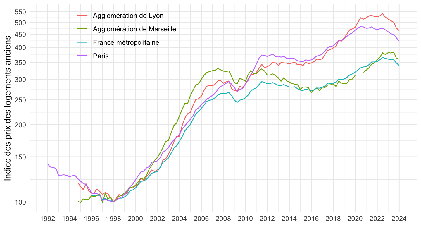
0612 - Indice des prix des produits médicaux divers
Code
"001763064+001763624" %>%
  paste0("https://www.bdm.insee.fr/series/sdmx/data/SERIES_BDM/", .) %>%
  readSDMX %>%
  as_tibble %>%
  month_to_date %>%
  mutate(OBS_VALUE = as.numeric(OBS_VALUE)) %>%
  filter(date >= as.Date("2018-01-01")) %>%
  arrange(date) %>%
  mutate(TITLE_FR = gsub("- Base 2015 - Ensemble des ménages ", "", TITLE_FR),
         TITLE_FR = gsub("- France - Nomenclature Coicop : ", "", TITLE_FR)) %>%
  group_by(TITLE_FR) %>%
  mutate(OBS_VALUE = 100*OBS_VALUE/OBS_VALUE[date == as.Date("2018-01-01")]) %>%
  ggplot() + ylab("") + xlab("") + theme_minimal() +
  geom_line(aes(x = date, y = OBS_VALUE, color = TITLE_FR)) +
  scale_x_date(breaks = seq(1920, 2100, 1) %>% paste0("-01-01") %>% as.Date,
               labels = date_format("%Y")) +
  theme(legend.position = c(0.4, 0.25),
        legend.title = element_blank()) +
  scale_y_log10(breaks = seq(10, 300, 5),
                     labels = dollar_format(accuracy = 1, prefix = ""))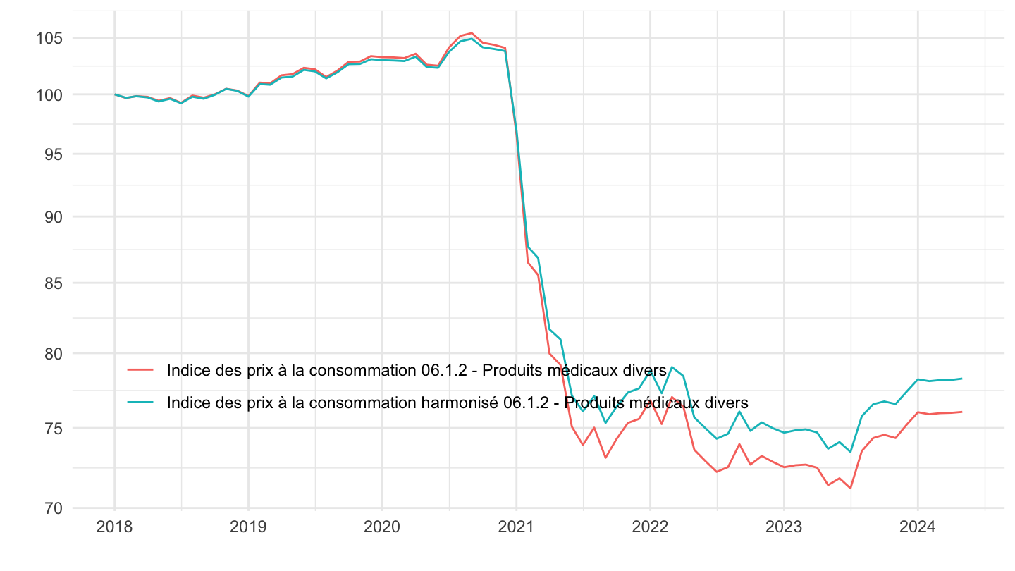
Biens, Biens et Services
Code
library("rsdmx")
library("tidyverse")
library("viridis")

"010565588+010565630+010565590+010565632+010565592+010565634+010565707" %>%
  paste0("https://www.bdm.insee.fr/series/sdmx/data/SERIES_BDM/", .) %>%
  readSDMX %>%
  as_tibble %>%
  mutate(OBS_VALUE = OBS_VALUE %>% as.numeric,
         year = TIME_PERIOD %>% substr(1, 4),
         month = (TIME_PERIOD %>% substr(7, 7) %>% as.numeric - 1)*3 + 1,
         month = month %>% str_pad(., 2, pad = "0"),
         date = paste0(year, "-", month, "-01") %>% as.Date) %>%
  select(IDBANK, date, OBS_VALUE) %>%
  spread(IDBANK, OBS_VALUE) %>%
  transmute(date,
            `Biens` = (`010565588` - `010565630`) / `010565707`,
            `Biens manufacturés ` = (`010565590` - `010565632`) / `010565707`,
            `Biens industriels` = (`010565592` - `010565634`) / `010565707`) %>%
  gather(Cna_produit, OBS_VALUE, -date) %>%
  ggplot + geom_line(aes(x = date, y = OBS_VALUE, color = Cna_produit)) +
  theme_minimal() + xlab("") + ylab("Exportations Nettes (% du PIB)") +
  scale_x_date(breaks = seq(1940, 2100, 10) %>% paste0("-01-01") %>% as.Date,
               labels = date_format("%Y")) +
  scale_y_continuous(breaks = 0.01*seq(-100, 500, 1),
                labels = percent_format(accuracy = 1)) +
  theme(legend.position = c(0.75, 0.9),
        legend.title = element_blank()) +
  geom_hline(yintercept = 0, linetype = "dashed")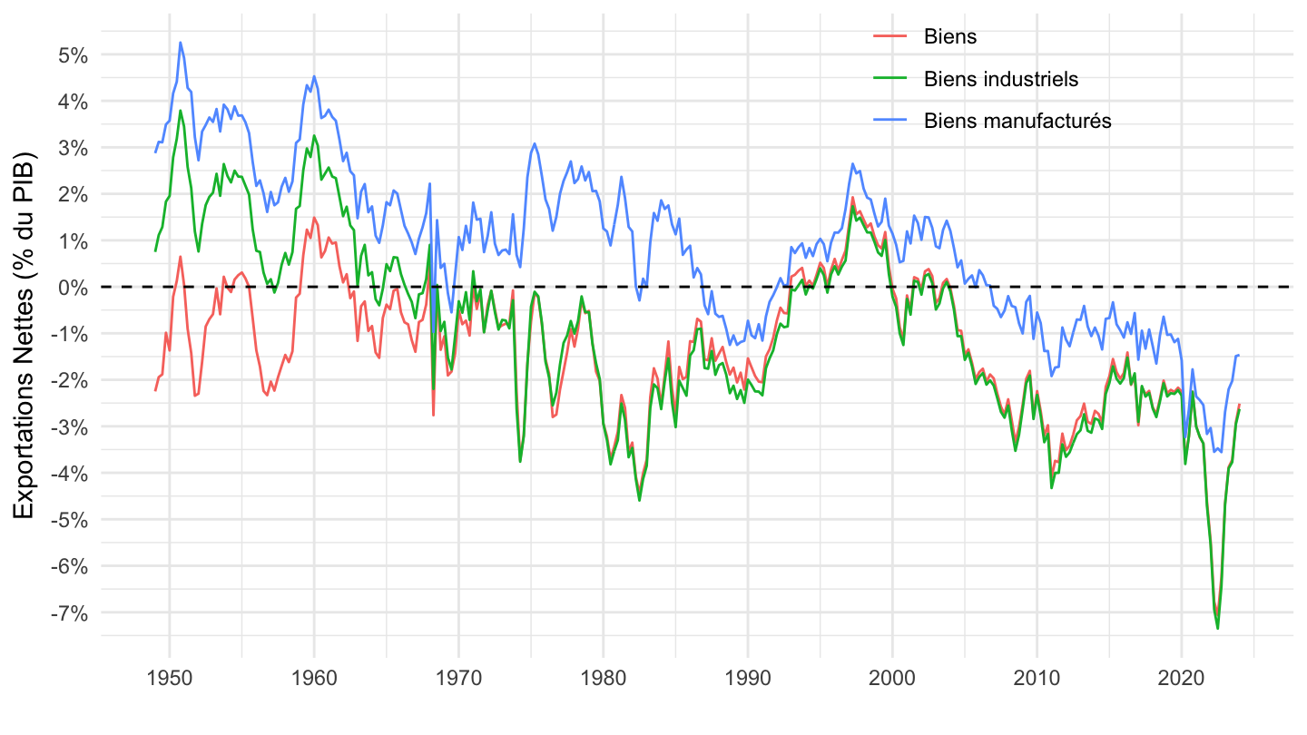
Emploi trimestriel
Code
library("rsdmx")
library("tidyverse")
library("zoo")
library("scales")
library("viridis")
"001791539+001791541+010599703+010600319" %>%
  paste0("https://www.bdm.insee.fr/series/sdmx/data/SERIES_BDM/", ., "?startPeriod=2016") %>%
  readSDMX %>%
  as_tibble %>%
  mutate(OBS_VALUE = OBS_VALUE %>% as.numeric,
         TIME_PERIOD = TIME_PERIOD %>% as.yearqtr(format = "%Y-Q%q") %>% as.Date) %>%
  group_by(TITLE_FR) %>%
  mutate(OBS_VALUE = 100*OBS_VALUE / OBS_VALUE[TIME_PERIOD == as.Date("2016-01-01")]) %>%
  ggplot + geom_line(aes(x = TIME_PERIOD, y = OBS_VALUE, color = TITLE_FR)) +
  scale_x_date(breaks = seq(1960, 2100, 1) %>% paste0("-01-01") %>% as.Date,
               labels = date_format("%Y")) +
  scale_y_log10(breaks = seq(0, 120, 1)) +
  xlab("") + ylab("Emploi Trimestriel (100 = 2016-Q1)") +  theme_minimal() +
  theme(legend.position = c(0.2, 0.9),
        legend.title = element_blank())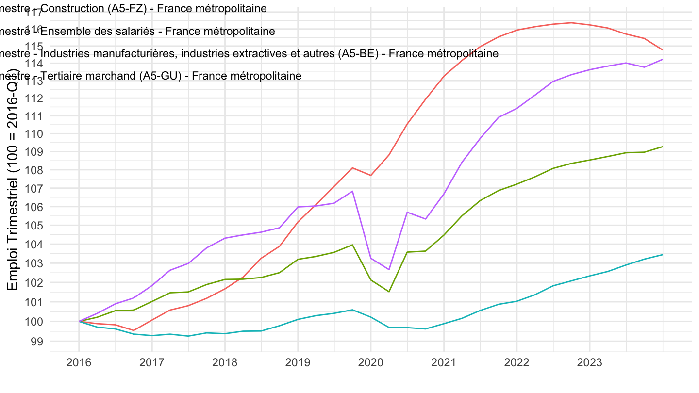
Calcul IRL
Code
"001763862" %>%
  paste0("https://www.bdm.insee.fr/series/sdmx/data/SERIES_BDM/", ., "?startPeriod=2006") %>%
  readSDMX %>%
  as_tibble %>%
  mutate(OBS_VALUE = OBS_VALUE %>% as.numeric,
         date = TIME_PERIOD %>% paste0("-01") %>% as.Date) %>%
  arrange(date) %>%
  transmute(date,
            `Inflation Indice de Référence des Loyers (IRL):\nVariation sur 12 mois de la moyenne sur 12 mois de l'IPC hors loyers, hors tabac` = zoo::rollmean(OBS_VALUE, 12, fill = NA, align = "right"),
            `Inflation Indice des Prix à la Consommation (IPC-) hors loyers, hors tabac: \nVariation sur 12 mois de l'IPC hors loyers, hors tabac` = OBS_VALUE) %>%
  filter(month(date) %in% c(12, 3, 6, 9)) %>%
  gather(variable, value, -date) %>%
  group_by(variable) %>%
  mutate(value_d12 = value/lag(value, 4) - 1) %>%
  na.omit %>%
  filter(date >= as.Date("2008-01-01")) %>%
  ggplot() + ylab("Inflation") + xlab("") + theme_minimal() +
  geom_line(aes(x = date, y = value_d12, color = variable)) +
  scale_color_manual(values = c("blue", "red")) +
  scale_x_date(breaks = seq(1920, 2100, 2) %>% paste0("-01-01") %>% as.Date,
               labels = date_format("%Y")) +
  theme(legend.position = c(0.45, 0.9),
        legend.title = element_blank(),
        legend.key.size= unit(1.0, 'cm')) +
  scale_y_continuous(breaks = 0.01*seq(-100, 300, 0.5),
                     labels = percent_format(accuracy = .1, prefix = ""))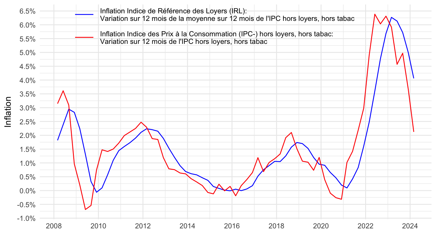
Calcul inflation annuelle pour pension de retraite
formule: croissance de la moyenne entre novembre Y-2 et octobre Y-1 pour la revalorisation du 1er janvier 2023 (001763852)
Code
"001763852" %>%
  paste0("https://www.bdm.insee.fr/series/sdmx/data/SERIES_BDM/", ., "?startPeriod=2006") %>%
  readSDMX %>%
  as_tibble %>%
  mutate(OBS_VALUE = OBS_VALUE %>% as.numeric,
         date = TIME_PERIOD %>% paste0("-01") %>% as.Date) %>%
  select(date, OBS_VALUE) %>%
  mutate(date2 = date + months(2),
         year = year(date2)) %>%
  group_by(year) %>%
  summarise(Nobs = n(),
            avg = mean(OBS_VALUE)) %>%
  mutate(date = as.Date(paste0(year, "-01-01")),
         OBS_VALUE = avg/lag(avg)-1) %>%
  ggplot() + ylab("croissance de la moyenne entre novembre Y-2 et octobre Y-1\n et novembre Y-1 et octobre Y") + xlab("") + theme_minimal() +
  geom_line(aes(x = date, y = OBS_VALUE)) +
  scale_x_date(breaks = seq(1920, 2100, 2) %>% paste0("-01-01") %>% as.Date,
               labels = date_format("%Y")) +
  scale_y_continuous(breaks = 0.01*seq(-100, 300, 0.5),
                     labels = percent_format(accuracy = .1, prefix = ""))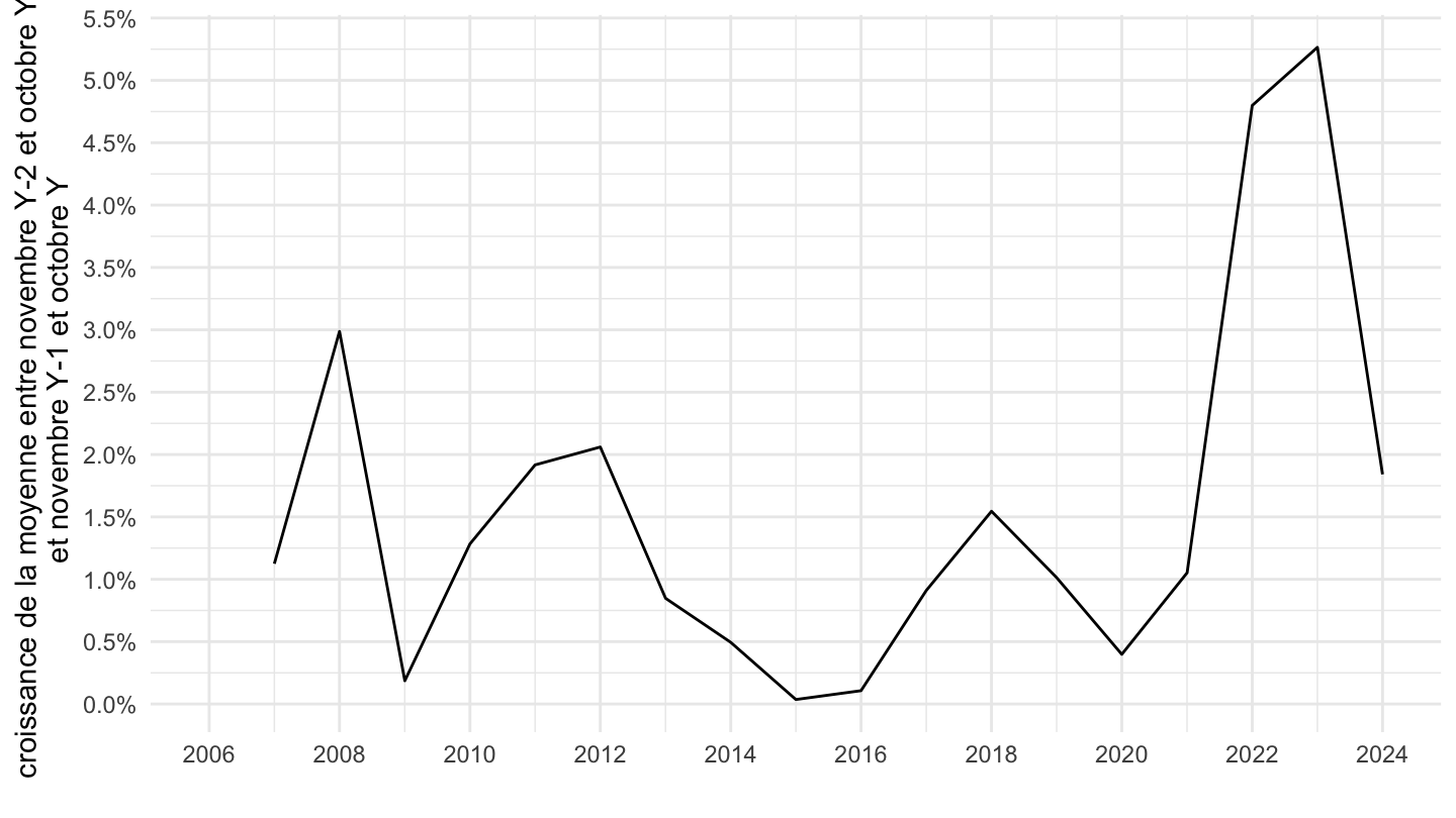
Glissement annuel inflation
Code
inflation_ga <- "001761313" %>%
  paste0("https://www.bdm.insee.fr/series/sdmx/data/SERIES_BDM/", ., "?startPeriod=2008") %>%
  readSDMX %>%
  as_tibble %>%
  mutate(OBS_VALUE = OBS_VALUE %>% as.numeric,
         date = TIME_PERIOD %>% paste0("-01") %>% as.Date) %>%
  transmute(date = TIME_PERIOD %>% paste0("-01") %>% as.Date,
            OBS_VALUE = OBS_VALUE %>% as.numeric/100,
            variable = "Glissement annuel (inflation)") %>%
  filter(month(date) == 1)

inflation_ga %>%
  ggplot() + ylab("Inflation") + xlab("") + theme_minimal() +
  geom_line(aes(x = date, y = OBS_VALUE, color = variable)) +
  scale_color_manual(values = c("blue", "red")) +
  scale_x_date(breaks = seq(1920, 2100, 2) %>% paste0("-01-01") %>% as.Date,
               labels = date_format("%Y")) +
  theme(legend.position = c(0.45, 0.9),
        legend.title = element_blank(),
        legend.key.size= unit(1.0, 'cm')) +
  scale_y_continuous(breaks = 0.01*seq(-100, 300, 0.5),
                     labels = percent_format(accuracy = .1, prefix = ""))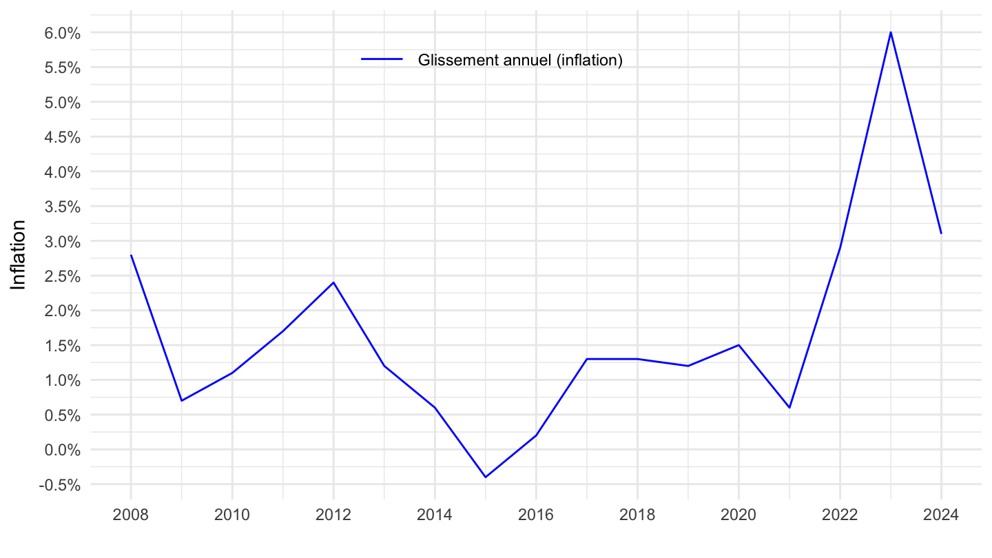
INSEE Package
Idbank list
Code
get_idbank_list() %>%
  head(100) %>%
  print_table_conditional
Dataset list
Code
get_dataset_list() %>%
  print_table_conditional
French GDP growth rate, quarter-on-quarter, sa-wda
Code
dataset_list = get_dataset_list()

df_idbank_list_selected =
  get_idbank_list("CNT-2014-PIB-EQB-RF") %>% # Gross domestic product balance
  filter(FREQ == "T") %>% #quarter
  add_insee_title() %>% #add titles
  filter(OPERATION == "PIB") %>% #GDP
  filter(NATURE == "TAUX") %>% #rate
  filter(CORRECTION == "CVS-CJO") #SA-WDA, seasonally adjusted, working day adjusted
#
|
| | 0%
|
|= | 2%
|
|== | 3%
|
|=== | 5%
|
|==== | 6%
|
|===== | 8%
|
|====== | 9%
|
|======= | 11%
|
|======== | 12%
|
|========== | 14%
|
|=========== | 15%
|
|============ | 17%
|
|============= | 18%
|
|============== | 20%
|
|=============== | 21%
|
|================ | 23%
|
|================= | 24%
|
|================== | 26%
|
|=================== | 27%
|
|==================== | 29%
|
|===================== | 30%
|
|====================== | 32%
|
|======================= | 33%
|
|======================== | 35%
|
|========================= | 36%
|
|=========================== | 38%
|
|============================ | 39%
|
|============================= | 41%
|
|============================== | 42%
|
|=============================== | 44%
|
|================================ | 45%
|
|================================= | 47%
|
|================================== | 48%
|
|=================================== | 50%
|
|==================================== | 52%
|
|===================================== | 53%
|
|====================================== | 55%
|
|======================================= | 56%
|
|======================================== | 58%
|
|========================================= | 59%
|
|========================================== | 61%
|
|=========================================== | 62%
|
|============================================= | 64%
|
|============================================== | 65%
|
|=============================================== | 67%
|
|================================================ | 68%
|
|================================================= | 70%
|
|================================================== | 71%
|
|=================================================== | 73%
|
|==================================================== | 74%
|
|===================================================== | 76%
|
|====================================================== | 77%
|
|======================================================= | 79%
|
|======================================================== | 80%
|
|========================================================= | 82%
|
|========================================================== | 83%
|
|=========================================================== | 85%
|
|============================================================ | 86%
|
|============================================================== | 88%
|
|=============================================================== | 89%
|
|================================================================ | 91%
|
|================================================================= | 92%
|
|================================================================== | 94%
|
|=================================================================== | 95%
|
|==================================================================== | 97%
|
|===================================================================== | 98%
|
|======================================================================| 100%Code
idbank = df_idbank_list_selected %>% pull(idbank)

data =
  get_insee_idbank(idbank)
#
|
| | 0%
|
|======================================================================| 100%Code
ggplot(data, aes(x = DATE, y = OBS_VALUE)) +
  geom_col() +
  ggtitle("French GDP growth rate, quarter-on-quarter, sa-wda") +
  labs(subtitle = sprintf("Last updated : %s", data$TIME_PERIOD[1]))
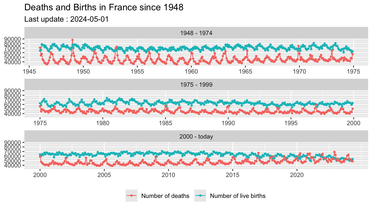
Deaths and Births in France since 1948
Code
insee_dataset = get_dataset_list()

list_idbank_selected =
  get_idbank_list("DECES-MORTALITE", "NAISSANCES-FECONDITE") %>%
  filter(FREQ == "M") %>% #monthly
  filter(REF_AREA == "FM") %>% #metropolitan territory
  filter(DEMOGRAPHIE %in% c("NAISS", "DECES"))

idbank_selected = list_idbank_selected %>% pull(idbank)

data =
  get_insee_idbank(idbank_selected) %>%
  split_title() %>%
  mutate(period = case_when(DATE < "1975-01-01" ~ "1948 - 1974",
                            DATE >= "1975-01-01" & DATE < "2000-01-01" ~ "1975 - 1999",
                            DATE >= "2000-01-01" ~ "2000 - today"
                            ))
#
|
| | 0%
|
|=================================== | 50%
|
|======================================================================| 100%Code
x_dates = seq.Date(from = as.Date("1940-01-01"), to = Sys.Date(), by = "5 years")
last_date = data %>% pull(DATE) %>% max()

ggplot(data, aes(x = DATE, y = OBS_VALUE, colour = TITLE_EN2)) +
  facet_wrap(~period, scales = "free_x", ncol = 1) +
  geom_line() +
  geom_point(size = 0.9) +
  ggtitle("Deaths and Births in France since 1948") +
  labs(subtitle = sprintf("Last update : %s", last_date)) +
  scale_x_date(breaks = x_dates, date_labels = "%Y") +
  theme(
    legend.position = "bottom",
    legend.title = element_blank(),
    axis.title.x = element_blank(),
    axis.title.y = element_blank()
    )
Information
INDICATEUR
Code
"https://www.bdm.insee.fr/series/sdmx/codelist/FR1/CL_INDICATEUR" %>%
  readSDMX() %>%
  as_tibble %>%
  select(1, 3) %>%
  {if (is_html_output()) datatable(., filter = 'top', rownames = F) else .}
Data Structure Definition (DSD)
Data Structure Definition: https://bdm.insee.fr/series/sdmx/ressource/agence/identifiant/version?parametresFacultatifs.
Example for CNA-2010-FBCF-SI: https://www.bdm.insee.fr/series/sdmx/datastructure/FR1/CNA-2010-FBCF-SI.
CNA-2010-FBCF-SI Components in DSD:
Code
"https://www.bdm.insee.fr/series/sdmx/datastructure/FR1/CNA-2010-FBCF-SI" %>%
  readSDMX() %>%
  slot("datastructures") %>%
  magrittr::extract2(1) %>%
  slot("Components") %>%
  as_tibble %>%
  select(1:4, 7) %>%
{if (is_html_output()) datatable(., filter = 'top', rownames = F) else .}- IPC-2015
Code
"https://www.bdm.insee.fr/series/sdmx/datastructure/FR1/IPC-2015" %>%
  readSDMX() %>%
  slot("datastructures") %>%
  magrittr::extract2(1) %>%
  slot("Components") %>%
  as_tibble %>%
  select(1:4, 7) %>%
  {if (is_html_output()) datatable(., filter = 'top', rownames = F) else .}
Using IDBANKS and startPeriod
Example 1
Code
"001565183+001690224+000067677" %>%
  paste0("https://www.bdm.insee.fr/series/sdmx/data/SERIES_BDM/", ., "?startPeriod=2010") %>%
  readSDMX %>%
  as_tibble %>%
  select(1, 3, TIME_PERIOD, OBS_VALUE) %>%
  head(10) %>%
{if (is_html_output()) print_table(.) else .}| IDBANK | TITLE_FR | TIME_PERIOD | OBS_VALUE |
|---|---|---|---|
| 001690224 | Produit intérieur brut total - Volume aux prix de l'année précédente chaînés - Série CVS-CJO - série arrêtée | 2018-Q1 | 547289 |
| 001690224 | Produit intérieur brut total - Volume aux prix de l'année précédente chaînés - Série CVS-CJO - série arrêtée | 2017-Q4 | 545905 |
| 001690224 | Produit intérieur brut total - Volume aux prix de l'année précédente chaînés - Série CVS-CJO - série arrêtée | 2017-Q3 | 542169 |
| 001690224 | Produit intérieur brut total - Volume aux prix de l'année précédente chaînés - Série CVS-CJO - série arrêtée | 2017-Q2 | 539312 |
| 001690224 | Produit intérieur brut total - Volume aux prix de l'année précédente chaînés - Série CVS-CJO - série arrêtée | 2017-Q1 | 535988 |
| 001690224 | Produit intérieur brut total - Volume aux prix de l'année précédente chaînés - Série CVS-CJO - série arrêtée | 2016-Q4 | 532264 |
| 001690224 | Produit intérieur brut total - Volume aux prix de l'année précédente chaînés - Série CVS-CJO - série arrêtée | 2016-Q3 | 529801 |
| 001690224 | Produit intérieur brut total - Volume aux prix de l'année précédente chaînés - Série CVS-CJO - série arrêtée | 2016-Q2 | 528970 |
| 001690224 | Produit intérieur brut total - Volume aux prix de l'année précédente chaînés - Série CVS-CJO - série arrêtée | 2016-Q1 | 529430 |
| 001690224 | Produit intérieur brut total - Volume aux prix de l'année précédente chaînés - Série CVS-CJO - série arrêtée | 2015-Q4 | 526173 |
Chômage Trimestriel
Code
`CHOMAGE-TRIM-NATIONAL` <- "CHOMAGE-TRIM-NATIONAL" %>%
  paste0("https://bdm.insee.fr/series/sdmx/data/", .) %>%
  readSDMX %>%
  as_tibble %>%
  select(IDBANK, TIME_PERIOD, OBS_VALUE)

`CHOMAGE-TRIM-NATIONAL` %>%
  head(10) %>%
{if (is_html_output()) print_table(.) else .}| IDBANK | TIME_PERIOD | OBS_VALUE |
|---|---|---|
| 001688370 | 2019-Q2 | 300 |
| 001688370 | 2019-Q1 | 314 |
| 001688370 | 2018-Q4 | 291 |
| 001688370 | 2018-Q3 | 352 |
| 001688370 | 2018-Q2 | 325 |
| 001688370 | 2018-Q1 | 313 |
| 001688370 | 2017-Q4 | 323 |
| 001688370 | 2017-Q3 | 345 |
| 001688370 | 2017-Q2 | 348 |
| 001688370 | 2017-Q1 | 327 |