| source | dataset | Title | Updated |
|---|---|---|---|
 bdf bdf |
api | Banque de France's API - api | 2026-10-06 |
 bea bea |
api | Bureau of Economic Analysis' API - api | 2026-10-06 |
 bis bis |
api | Bank of International Settlements' API - api | 2026-10-06 |
 bls bls |
api | Bureau of Labor Statistics' API - api | 2026-10-06 |
 dbnomics dbnomics |
api | DBnomics' API - api | 2026-10-04 |
 ecb ecb |
api | European Central Bank's API - api | 2026-10-01 |
 eurostat eurostat |
api | Eurostat's API - api | 2026-10-06 |
 imf imf |
api | International Monetary Fund's API - api | 2026-10-06 |
 insee insee |
api | Institut National de la Statistique et des Etudes Economiques' API - api | 2026-10-04 |
 oecd oecd |
api | OECD's API - api | 2026-08-02 |
 wdi wdi |
api | World Development Indicators' API - api | 2026-10-06 |
Info
List of APIs
All
LAST_COMPILE
| LAST_COMPILE |
|---|
| 2026-10-07 |
Nominal GDP
Code
rdb(ids = c("OECD/QNA/FRA.B1_GE.CARSA.Q",
            "OECD/QNA/USA.B1_GE.CARSA.Q",
            "OECD/QNA/ITA.B1_GE.CARSA.Q",
            "OECD/QNA/GBR.B1_GE.CARSA.Q",
            "OECD/QNA/ESP.B1_GE.CARSA.Q",
            "OECD/QNA/DEU.B1_GE.CARSA.Q")) |>
  filter(period >= as.Date("2019-10-01")) |>
  select(Country, period, value) |>
  group_by(Country) |>
  mutate(value = 100*value/value[1]) |>
  ggplot() + geom_line(aes(x = period, y = value, color = Country)) +
  theme_minimal() + xlab("") + ylab("Real GDP") +
  theme(legend.position = c(0.85, 0.3),
        legend.title = element_blank(),
        axis.text.x = element_text(angle = 45, vjust = 1, hjust = 1)) +
  scale_x_date(breaks = "3 months",
               labels = date_format("%m-%Y")) +
  scale_y_continuous(breaks = seq(80, 200, 2))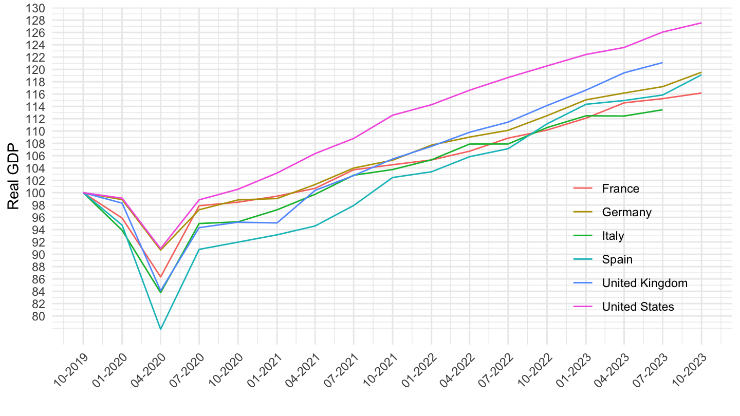
Real GDP
Code
rdb(ids = c("OECD/QNA/FRA.B1_GE.VOBARSA.Q",
            "OECD/QNA/USA.B1_GE.VOBARSA.Q",
            "OECD/QNA/ITA.B1_GE.VOBARSA.Q",
            "OECD/QNA/GBR.B1_GE.VOBARSA.Q",
            "OECD/QNA/ESP.B1_GE.VOBARSA.Q",
            "OECD/QNA/DEU.B1_GE.VOBARSA.Q")) |>
  filter(period >= as.Date("2019-10-01")) |>
  select(Country, period, value) |>
  group_by(Country) |>
  mutate(value = 100*value/value[1]) |>
  ggplot() + geom_line(aes(x = period, y = value, color = Country)) +
  theme_minimal() + xlab("") + ylab("Real GDP") +
  theme(legend.position = c(0.85, 0.3),
        legend.title = element_blank(),
        axis.text.x = element_text(angle = 45, vjust = 1, hjust = 1)) +
  scale_x_date(breaks = "3 months",
               labels = date_format("%m-%Y")) +
  scale_y_continuous(breaks = seq(80, 120, 2))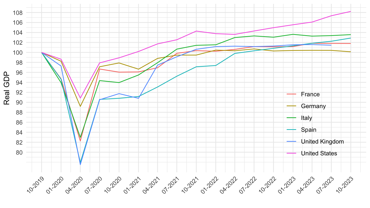
U.S. Real GDP Cycle
Code
rdb(ids = "BEA/NIPA-T10106/A191RX-A") |>
  select(date = period, `Real GDP` = value) |>
  mutate(year = lubridate::year(date)) |>
  mutate(`HP (1000) Cycle` = exp(hpfilter(log(`Real GDP`), freq = 1000,
                                          type = "lambda", drift = FALSE)$cycle),
         `HP (10000) Cycle` = exp(hpfilter(log(`Real GDP`), freq = 10000,
                                           type = "lambda", drift = FALSE)$cycle),
         `Log-Linear Cycle` = exp(residuals(lm(log(`Real GDP`) ~ year,
                                               na.action = na.exclude)))) |>
  group_by(date) |>
  select(-year, - `Real GDP`) |>
  gather(variable, value, -date) |>
  ggplot() + geom_line(aes(x = date, y = value, linetype = variable)) +
  theme_minimal() +
  theme(legend.title = element_blank(),
        legend.position = c(0.8, 0.8)) +
  geom_rect(data = nber_recessions |>
              filter(Peak > as.Date("1928-01-01")),
            aes(xmin = Peak, xmax = Trough, ymin = -Inf, ymax = +Inf),
            fill = 'grey', alpha = 0.5) +
  scale_x_date(breaks = nber_recessions$Peak,
               labels = date_format("%Y")) +
  scale_y_continuous(breaks = seq(0.60, 1.40, 0.05),
                     labels = scales::percent_format(accuracy = 1)) +
  xlab("") + ylab("GDP Cycle (% of Trend)")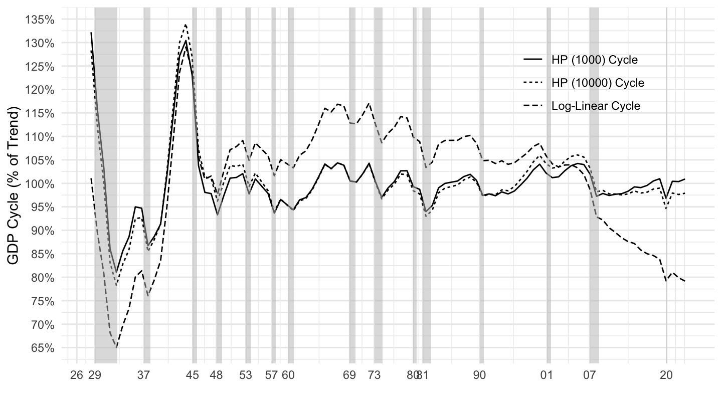
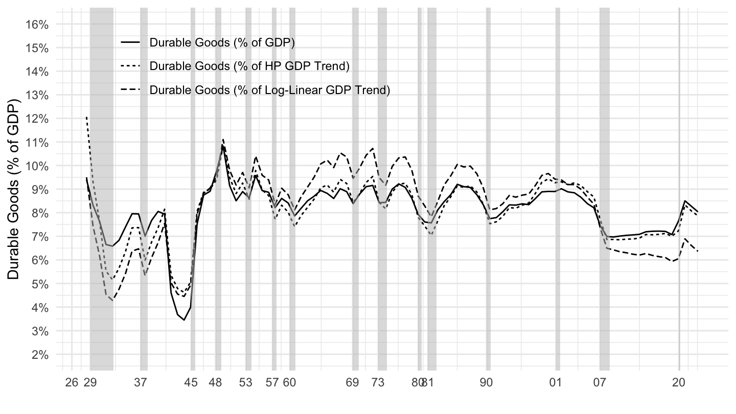
U.S. Durable Goods
Code
rdb(ids = c("BEA/NIPA-T10106/A191RX-A",
            "BEA/NIPA-T10105/DDURRC-A",
            "BEA/NIPA-T10105/A191RC-A")) |>
  select(series_code, date = period, value) |>
  spread(series_code, value) |>
  rename(GDP = `A191RC-A`,
         `Durable Goods` = `DDURRC-A`,
         `Real GDP` = `A191RX-A`) |>
  mutate(year = lubridate::year(date),
         `Real GDP HP (10000) Trend` = exp(hpfilter(log(`Real GDP`), freq = 10000,
                                                    type = "lambda", drift = FALSE)$trend),
         `Real GDP Log-Linear Trend` = exp(fitted(lm(log(`Real GDP`) ~ year,
                                                     na.action = na.exclude))),
         `Durable Goods (% of GDP)` = `Durable Goods` / GDP,
         `Durable Goods (% of Log-Linear GDP Trend)` =
           (`Durable Goods` / GDP)*(`Real GDP` / `Real GDP Log-Linear Trend`),
         `Durable Goods (% of HP GDP Trend)` =
           (`Durable Goods` / GDP)*(`Real GDP` / `Real GDP HP (10000) Trend`)) |>
  select(date, contains("Durable Goods (%")) |>
  gather(variable, value, -date) |>
  ggplot() +
  geom_line(aes(x = date, y = value, linetype = variable)) +
  theme_minimal() +
  theme(legend.title = element_blank(),
        legend.position = c(0.3, 0.85)) +
  geom_rect(data = nber_recessions |>
              filter(Peak >= as.Date("1928-01-01")),
            aes(xmin = Peak, xmax = Trough, ymin = -Inf, ymax = +Inf),
            fill = 'grey', alpha = 0.5) +
  scale_x_date(breaks = nber_recessions$Peak,
               labels = date_format("%Y")) +
  scale_y_continuous(breaks = 0.01*seq(2, 16, 1),
                     limits = 0.01*c(2, 16),
                     labels = scales::percent_format(accuracy = 1)) +
  xlab("") + ylab("Durable Goods (% of GDP)")