
Last observation: juil. 2026 (N = 25777)
First observation: janv. 1991 (N = 2482)
Last data update: 20 sept. 2026, 22:24
Last compile: 06 oct. 2026, 04:55
bop_c6_m |>
  filter(geo %in% c("DE", "FR", "IT"),
         stk_flow == "BAL",
         currency == "MIO_EUR",
         partner == "WRL_REST",
         bop_item == "CA") |>
  month_to_date() |>

  left_join(B1GQ, by = c("geo", "date")) |>
  group_by(Geo) |>
  arrange(date) |>
  mutate(B1GQ_i = spline(x = date, y = B1GQ, xout = date)$y,
         values = 3*values / B1GQ_i) |>
  add_flag_color("Geo") |>
  ggplot() + geom_line(aes(x = date, y = values, color = color)) +
  scale_color_identity() + add_flags +
  scale_color_manual(values = c("#002395", "#000000", "#009246")) +
  theme_minimal()  +
  scale_x_date(breaks = as.Date(paste0(seq(1960, 2100, 5), "-01-01")),
               labels = date_format("%Y")) +
  geom_image(data = . %>%
               filter(date == as.Date("2008-01-01")) %>%
               mutate(image = paste0("../../icon/flag/", str_to_lower(Geo), ".png")),
             aes(x = date, y = values, image = image), asp = 1.5) +
  theme(legend.position = "none") +
  xlab("") + ylab("") +
  scale_y_continuous(breaks = 0.01*seq(-30, 30, 1),
                labels = percent_format(a = 1)) +
  geom_hline(yintercept = 0, linetype = "dashed",  color = "black")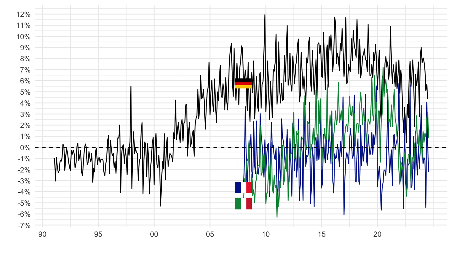
bop_c6_m |>
  filter(geo %in% c("DE", "FR", "IT"),
         stk_flow == "BAL",
         currency == "MIO_EUR",
         partner == "WRL_REST",
         bop_item == "KA") |>
  month_to_date() |>

  left_join(B1GQ, by = c("geo", "date")) |>
  group_by(Geo) |>
  arrange(date) |>
  mutate(B1GQ_i = spline(x = date, y = B1GQ, xout = date)$y,
         values = 3*values / B1GQ_i) |>
  add_flag_color("Geo") |>
  ggplot() + geom_line(aes(x = date, y = values, color = color)) +
  scale_color_identity() + add_flags +
  scale_color_manual(values = c("#002395", "#000000", "#009246")) +
  theme_minimal()  +
  scale_x_date(breaks = as.Date(paste0(seq(1960, 2100, 5), "-01-01")),
               labels = date_format("%Y")) +
  geom_image(data = . %>%
               filter(date == as.Date("2008-01-01")) %>%
               mutate(image = paste0("../../icon/flag/", str_to_lower(Geo), ".png")),
             aes(x = date, y = values, image = image), asp = 1.5) +
  theme(legend.position = "none") +
  xlab("") + ylab("") +
  scale_y_continuous(breaks = 0.01*seq(-30, 30, 1),
                labels = percent_format(a = 1)) +
  geom_hline(yintercept = 0, linetype = "dashed",  color = "black")
bop_c6_m |>
  filter(geo %in% c("DE", "FR", "IT"),
         stk_flow == "NET",
         currency == "MIO_EUR",
         partner == "WRL_REST",
         bop_item == "FA") |>
  month_to_date() |>

  left_join(B1GQ, by = c("geo", "date")) |>
  group_by(Geo) |>
  arrange(date) |>
  mutate(B1GQ_i = spline(x = date, y = B1GQ, xout = date)$y,
         values = 3*values / B1GQ_i) |>
  add_flag_color("Geo") |>
  ggplot() + geom_line(aes(x = date, y = values, color = color)) +
  scale_color_identity() + add_flags +
  scale_color_manual(values = c("#002395", "#000000", "#009246")) +
  theme_minimal()  +
  scale_x_date(breaks = as.Date(paste0(seq(1960, 2100, 5), "-01-01")),
               labels = date_format("%Y")) +
  geom_image(data = . %>%
               filter(date == as.Date("2008-01-01")) %>%
               mutate(image = paste0("../../icon/flag/", str_to_lower(Geo), ".png")),
             aes(x = date, y = values, image = image), asp = 1.5) +
  theme(legend.position = "none") +
  xlab("") + ylab("") +
  scale_y_continuous(breaks = 0.01*seq(-30, 30, 2),
                labels = percent_format(a = 1)) +
  geom_hline(yintercept = 0, linetype = "dashed",  color = "black")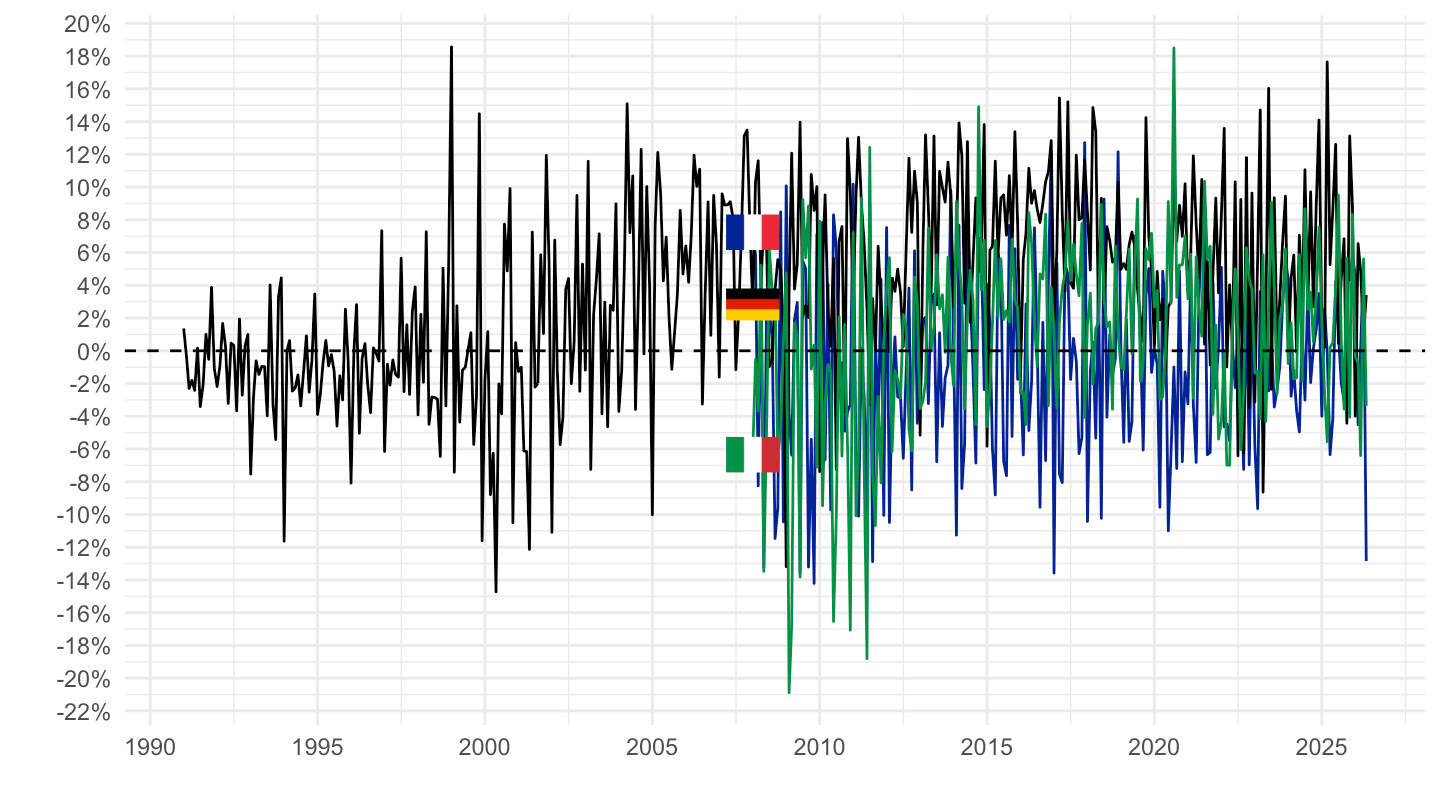
latest_m <- bop_c6_m |>
  filter(bop_item == "CA",
         stk_flow == "BAL",
         partner == "WRL_REST",
         sector10 == "S1",
         sectpart == "S1",
         currency == "MIO_EUR",
         geo %in% c("DE", "FR", "IT", "ES", "NL", "BE", "PT", "IE"),
         !is.na(values)) |>
  summarise(m = max(time)) |>
  pull(m)

bop_c6_m |>
  filter(geo %in% c("DE", "FR", "IT", "ES", "NL", "BE", "PT", "IE"),
         stk_flow == "BAL",
         partner == "WRL_REST",
         sector10 == "S1",
         sectpart == "S1",
         currency == "MIO_EUR",
         bop_item %in% c("CA", "KA", "FA", "G", "S", "GS", "IN1", "IN2"),
         time == latest_m) |>
  mutate(values = values/1000) |>
  select(bop_item, Bop_item, Geo, values) |>
  spread(Geo, values) |>
print_table_conditional()| bop_item | Bop_item | Belgium | France | Germany | Ireland | Italy | Netherlands | Portugal | Spain |
|---|---|---|---|---|---|---|---|---|---|
| CA | Current account | 0.887 | -5.252 | 21.154 | NA | 7.384 | NA | 0.828 | NA |
| G | Goods | 2.001 | -5.121 | 21.062 | NA | 8.189 | NA | -2.775 | NA |
| GS | Goods and services | 0.701 | -0.850 | 12.775 | NA | 9.291 | NA | 0.868 | NA |
| IN1 | Primary income | 1.049 | 1.186 | 15.043 | NA | -0.116 | NA | -0.395 | NA |
| IN2 | Secondary income | -0.864 | -5.588 | -6.665 | NA | -1.791 | NA | 0.355 | NA |
| KA | Capital account | -0.501 | 0.383 | 2.164 | NA | 0.192 | NA | 0.368 | NA |
| S | Services | -1.300 | 4.271 | -8.288 | NA | 1.103 | NA | 3.642 | NA |
bop_c6_m |>
  filter(geo == "FR",
         stk_flow == "BAL",
         time == "2021M04",
         currency == "MIO_EUR",
         partner %in% c("EA19", "EXT_EA19", "WRL_REST")) |>

  select(bop_item, Bop_item, everything()) %>%
  select_if(~n_distinct(.) > 1) |>
  spread(partner, values) |>
  arrange(sector10) |>
print_table_conditional()bop_c6_m |>
filter(geo == "DE",
stk_flow == "BAL",
time == "2021M04",
currency == "MIO_EUR",
partner %in% c("EA19", "EXT_EA19", "WRL_REST")) |>
select(bop_item, Bop_item, everything()) %>%
select_if(~n_distinct(.) > 1) |>
spread(partner, values) |>
arrange(sector10) |>
print_table_conditional()bop_c6_m |>
filter(geo == "FR",
stk_flow == "BAL",
time == "2021M04",
currency == "MIO_EUR",
partner %in% c("EA19", "EXT_EA19", "WRL_REST")) |>
select(bop_item, Bop_item, everything()) %>%
select_if(~n_distinct(.) > 1) |>
spread(partner, values) |>
arrange(sector10) |>
print_table_conditional()bop_c6_m |>
filter(geo == "DE",
stk_flow == "BAL",
time == "2021M04",
currency == "MIO_EUR",
partner %in% c("EA19", "EXT_EA19", "WRL_REST")) |>
select(bop_item, Bop_item, everything()) %>%
select_if(~n_distinct(.) > 1) |>
spread(partner, values) |>
arrange(sector10) |>
print_table_conditional()