
Last observation: 2020 (N = 37)
First observation: 1985 (N = 20)
Last data update: 02 août 2026, 08:58
Last compile: 05 oct. 2026, 00:25
EO |>
  filter(LOCATION %in% c("FRA", "DEU", "ITA")) |>
  left_join(EO_var$LOCATION, by = "LOCATION") |>
  year_to_date() |>
  ggplot() + theme_minimal() + ylab("NAIRU, OECD (% of GDP)") + xlab("") +
  geom_line(aes(x = date, y = obsValue/100, color = Location)) +
  geom_image(data = . %>%
               filter(date == as.Date("2017-01-01")) %>%
               mutate(image = paste0("../../icon/flag/", str_to_lower(gsub(" ", "-", Location)), ".png")),
             aes(x = date, y = obsValue/100, image = image), asp = 1.5) +
  scale_color_manual(values = c("#0055a4", "#000000", "#008c45")) +
  scale_x_date(breaks = seq(1920, 2100, 5) |> paste0("-01-01") |> as.Date(),
               labels = date_format("%Y")) +
  theme(legend.position = c(0.15, 0.2),
        legend.title = element_blank()) +
  scale_y_continuous(breaks = 0.01*seq(-7, 60, 1),
                     labels = scales::percent_format(accuracy = 1))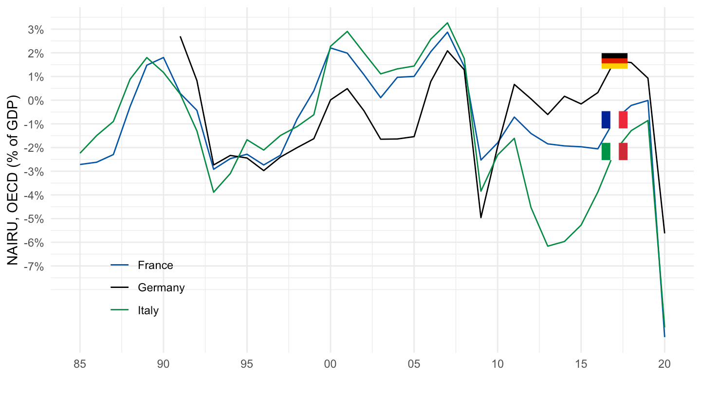
EO |>
  filter(LOCATION %in% c("FRA", "DEU", "ITA")) |>
  left_join(EO_var$LOCATION, by = "LOCATION") |>
  year_to_date() |>
  filter(date >= as.Date("1995-01-01")) |>
  ggplot() + theme_minimal() + ylab("NAIRU, OECD (% of GDP)") + xlab("") +
  geom_line(aes(x = date, y = obsValue/100, color = Location)) +
  geom_image(data = . %>%
               filter(date == as.Date("2017-01-01")) %>%
               mutate(image = paste0("../../icon/flag/", str_to_lower(gsub(" ", "-", Location)), ".png")),
             aes(x = date, y = obsValue/100, image = image), asp = 1.5) +
  scale_color_manual(values = c("#0055a4", "#000000", "#008c45")) +
  scale_x_date(breaks = seq(1920, 2100, 5) |> paste0("-01-01") |> as.Date(),
               labels = date_format("%Y")) +
  theme(legend.position = c(0.15, 0.2),
        legend.title = element_blank()) +
  scale_y_continuous(breaks = 0.01*seq(-7, 60, 1),
                     labels = scales::percent_format(accuracy = 1))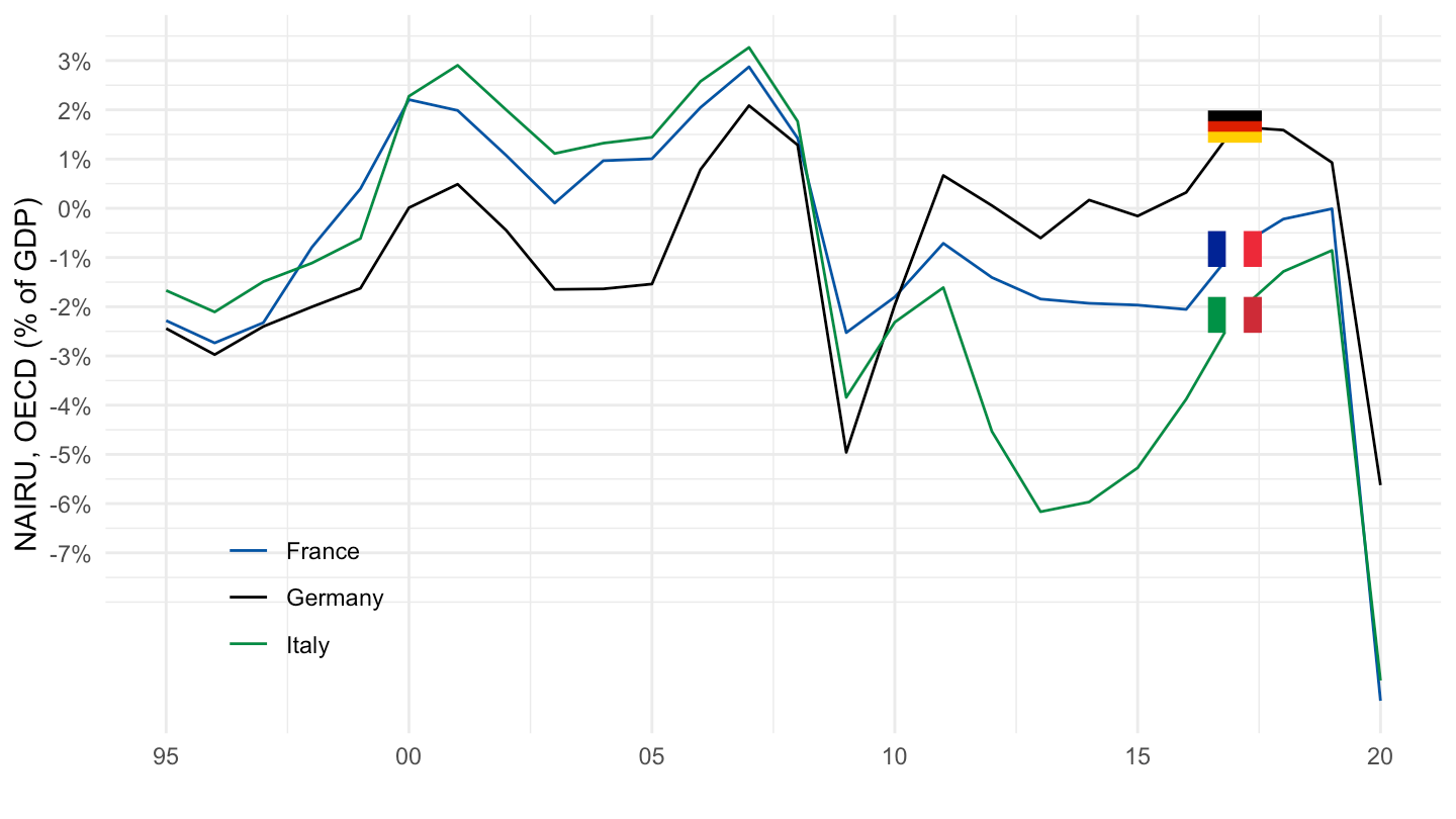
EO |>
  filter(LOCATION %in% c("USA", "GBR", "JPN")) |>
  left_join(EO_var$LOCATION, by = "LOCATION") |>
  year_to_date() |>
  ggplot() + theme_minimal() + ylab("NAIRU, OECD (% of GDP)") + xlab("") +
  geom_line(aes(x = date, y = obsValue/100, color = Location)) +
  geom_image(data = . %>%
               filter(date == as.Date("2017-01-01")) %>%
               mutate(image = paste0("../../icon/flag/", str_to_lower(gsub(" ", "-", Location)), ".png")),
             aes(x = date, y = obsValue/100, image = image), asp = 1.5) +
  scale_color_manual(values = c("#0055a4", "#000000", "#008c45")) +
  scale_x_date(breaks = seq(1920, 2100, 5) |> paste0("-01-01") |> as.Date(),
               labels = date_format("%Y")) +
  theme(legend.position = c(0.15, 0.2),
        legend.title = element_blank()) +
  scale_y_continuous(breaks = 0.01*seq(-7, 60, 1),
                     labels = scales::percent_format(accuracy = 1))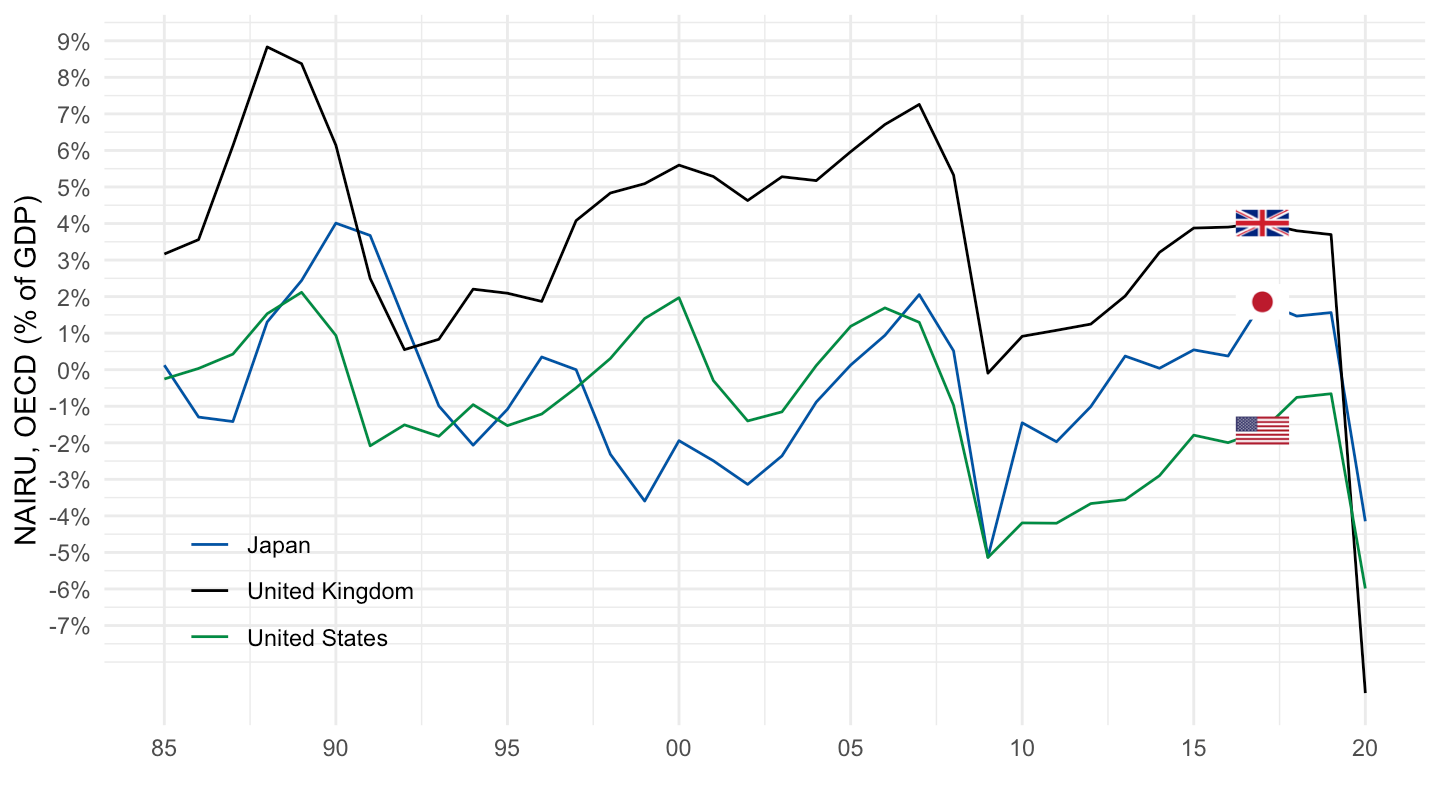
EO |>
  filter(LOCATION %in% c("EA17", "USA")) |>
  left_join(EO_var$LOCATION, by = "LOCATION") |>
  year_to_date() |>
  filter(!is.na(obsValue), date >= as.Date("1995-01-01")) |>
  mutate(Country = ifelse(LOCATION == "EA17", "Euro area", "United States")) |>
  ggplot() + theme_minimal() + xlab("") +
  ylab("Output gap (% of potential GDP)") +
  geom_hline(yintercept = 0, linewidth = 0.3) +
  geom_line(aes(x = date, y = obsValue / 100, color = Country)) +
  scale_color_manual(values = c("Euro area" = "#003399", "United States" = "#b22234")) +
  scale_x_date(breaks = seq(1920, 2100, 5) |> paste0("-01-01") |> as.Date(),
               labels = date_format("%Y")) +
  theme(legend.position = c(0.16, 0.18), legend.title = element_blank()) +
  scale_y_continuous(breaks = 0.01 * seq(-15, 15, 1),
                     labels = scales::percent_format(accuracy = 1))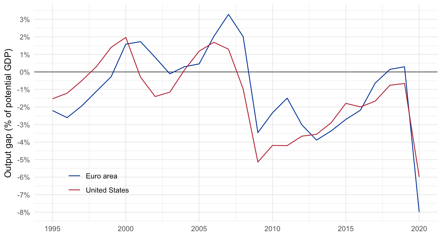
| source | dataset | Title | Updated |
|---|---|---|---|


