Code
tibble(LAST_DOWNLOAD = as.Date(file.info("~/iCloud/website/data/eurostat/ei_bsin_m_r2.RData")$mtime)) %>%
print_table_conditional()| LAST_DOWNLOAD |
|---|
| 2026-04-14 |
Data - Eurostat
tibble(LAST_DOWNLOAD = as.Date(file.info("~/iCloud/website/data/eurostat/ei_bsin_m_r2.RData")$mtime)) %>%
print_table_conditional()| LAST_DOWNLOAD |
|---|
| 2026-04-14 |
| LAST_COMPILE |
|---|
| 2026-07-22 |
ei_bsin_m_r2 %>%
  group_by(time) %>%
  summarise(Nobs = n()) %>%
  arrange(desc(time)) %>%
  head(1) %>%
print_table_conditional()| time | Nobs |
|---|---|
| 2026M03 | 544 |
ei_bsin_m_r2 %>%
  left_join(indic, by = "indic") %>%
  group_by(indic, Indic) %>%
  summarise(Nobs = n()) %>%
  arrange(-Nobs) %>%
print_table_conditional()| indic | Indic | Nobs |
|---|---|---|
| BS-IPE | Production expectations over the next 3 months | 28886 |
| BS-IPT | Production development observed over the past 3 months | 28718 |
| BS-IOB | Assessment of order-book levels | 28706 |
| BS-ISFP | Assessment of the current level of stocks of finished products | 28550 |
| BS-ICI | Industrial confidence indicator | 28370 |
| BS-IEOB | Assessment of export order-book levels | 28180 |
| BS-ISPE | Selling price expectations over the next 3 months | 27997 |
| BS-IEME-BAL | Employment expectations over the next 3 months - industry | 27740 |
| BS-IEME | Employment expectations over the next 3 months | 25358 |
ei_bsin_m_r2 %>%
  left_join(s_adj, by = "s_adj") %>%
  group_by(s_adj, S_adj) %>%
  summarise(Nobs = n()) %>%
  arrange(-Nobs) %>%
print_table_conditional()| s_adj | S_adj | Nobs |
|---|---|---|
| SA | Seasonally adjusted data, not calendar adjusted data | 126308 |
| NSA | Unadjusted data (i.e. neither seasonally adjusted nor calendar adjusted data) | 126197 |
ei_bsin_m_r2 %>%
  left_join(geo, by = "geo") %>%
  group_by(geo, Geo) %>%
  summarise(Nobs = n()) %>%
  arrange(-Nobs) %>%
  mutate(Geo = ifelse(geo == "DE", "Germany", Geo)) %>%
  mutate(Flag = gsub(" ", "-", str_to_lower(Geo)),
         Flag = paste0('<img src="../../bib/flags/vsmall/', Flag, '.png" alt="Flag">')) %>%
  select(Flag, everything()) %>%
{if (is_html_output()) datatable(., filter = 'top', rownames = F, escape = F) else .}ei_bsin_m_r2 %>%
group_by(time) %>%
summarise(Nobs = n()) %>%
print_table_conditional()ei_bsin_m_r2 %>%
filter(indic == "BS-IPE",
geo %in% c("FR", "DE", "IT"),
s_adj == "NSA") %>%
select(geo, time, values) %>%
left_join(geo, by = "geo") %>%
mutate(Geo = ifelse(geo == "DE", "Germany", Geo)) %>%
month_to_date %>%
left_join(colors, by = c("Geo" = "country")) %>%
ggplot() + ylab("Industrial confidence indicator") + xlab("") + theme_minimal() +
geom_line(aes(x = date, y = values, color = color)) +
scale_color_identity() + add_3flags + theme(legend.position = "none") +
scale_x_date(breaks = seq(1920, 2025, 5) %>% paste0("-01-01") %>% as.Date,
labels = date_format("%Y")) +
scale_y_continuous(breaks = seq(-2000, 2000, 5))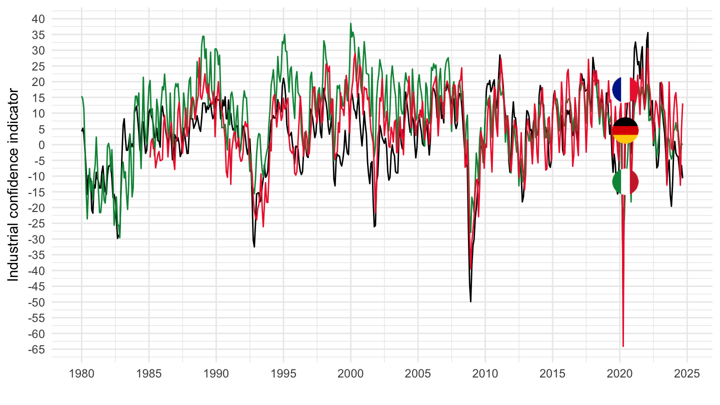
ei_bsin_m_r2 %>%
  filter(indic == "BS-IPE",
         geo %in% c("FR", "DE", "IT"),
         s_adj == "NSA") %>%
  select(geo, time, values) %>%
  group_by(geo) %>%
  left_join(geo, by = "geo") %>%
  mutate(Geo = ifelse(geo == "DE", "Germany", Geo)) %>%
  month_to_date %>%
  filter(date >= as.Date("1995-01-01")) %>%
  left_join(colors, by = c("Geo" = "country")) %>%
  ggplot() + ylab("Industrial confidence indicator") + xlab("") + theme_minimal() +
  geom_line(aes(x = date, y = values, color = color)) +
  scale_color_identity() + add_3flags + theme(legend.position = "none") +
  scale_x_date(breaks = seq(1920, 2025, 5) %>% paste0("-01-01") %>% as.Date,
               labels = date_format("%Y")) +
  scale_y_continuous(breaks = seq(-2000, 2000, 5))
ei_bsin_m_r2 %>%
  filter(indic == "BS-IPE",
         geo %in% c("FR", "DE", "IT"),
         s_adj == "NSA") %>%
  select(geo, time, values) %>%
  group_by(geo) %>%
  left_join(geo, by = "geo") %>%
  mutate(Geo = ifelse(geo == "DE", "Germany", Geo)) %>%
  month_to_date %>%
  filter(date >= as.Date("2000-01-01")) %>%
  left_join(colors, by = c("Geo" = "country")) %>%
  ggplot() + ylab("Industrial confidence indicator") + xlab("") + theme_minimal() +
  geom_line(aes(x = date, y = values, color = color)) +
  scale_color_identity() + add_3flags + theme(legend.position = "none") +
  scale_x_date(breaks = seq(1920, 2025, 5) %>% paste0("-01-01") %>% as.Date,
               labels = date_format("%Y")) +
  scale_y_continuous(breaks = seq(-2000, 2000, 5))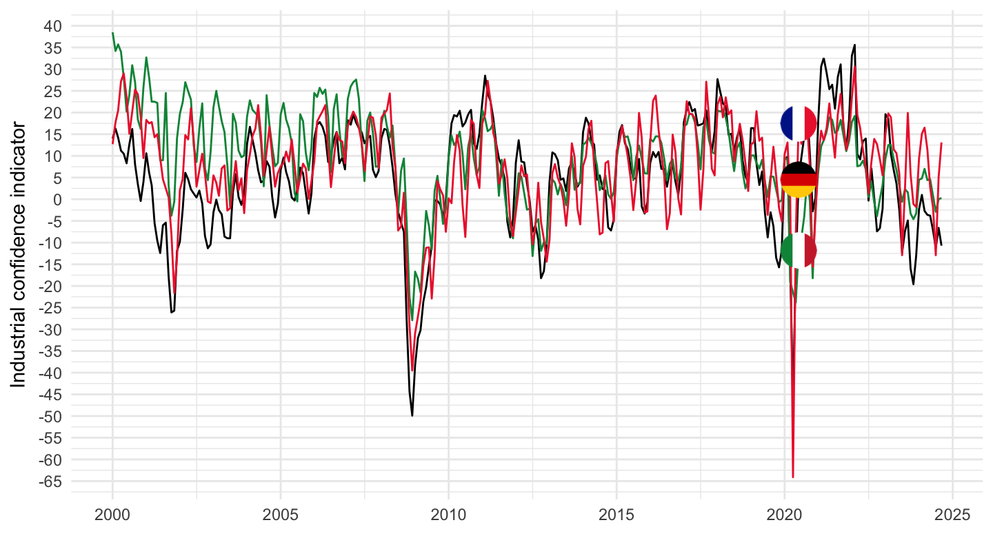
ei_bsin_m_r2 %>%
  filter(indic == "BS-IPE",
         geo %in% c("FR", "DE", "IT"),
         s_adj == "NSA") %>%
  select(geo, time, values) %>%
  group_by(geo) %>%
  left_join(geo, by = "geo") %>%
  mutate(Geo = ifelse(geo == "DE", "Germany", Geo)) %>%
  month_to_date %>%
  filter(date >= as.Date("2015-01-01")) %>%
  left_join(colors, by = c("Geo" = "country")) %>%
  ggplot() + ylab("Industrial confidence indicator") + xlab("") + theme_minimal() +
  geom_line(aes(x = date, y = values, color = color)) +
  scale_color_identity() + add_3flags + theme(legend.position = "none") +
  scale_x_date(breaks = seq(1920, 2025, 1) %>% paste0("-01-01") %>% as.Date,
               labels = date_format("%Y")) +
  scale_y_continuous(breaks = seq(-2000, 2000, 5))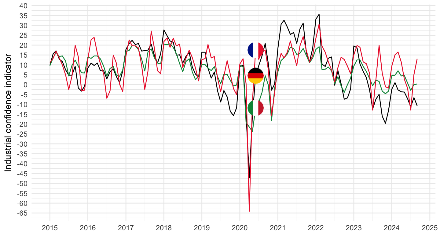
ei_bsin_m_r2 %>%
  filter(indic == "BS-ICI",
         geo %in% c("FR", "DE", "IT"),
         s_adj == "NSA") %>%
  select(geo, time, values) %>%
  left_join(geo, by = "geo") %>%
  mutate(Geo = ifelse(geo == "DE", "Germany", Geo)) %>%
  month_to_date %>%
  left_join(colors, by = c("Geo" = "country")) %>%
  ggplot() + ylab("Industrial confidence indicator") + xlab("") + theme_minimal() +
  geom_line(aes(x = date, y = values, color = color)) +
  scale_color_identity() + add_3flags + theme(legend.position = "none") +
  scale_x_date(breaks = seq(1920, 2025, 5) %>% paste0("-01-01") %>% as.Date,
               labels = date_format("%Y")) +
  scale_y_continuous(breaks = seq(-2000, 2000, 5))
ei_bsin_m_r2 %>%
  filter(indic == "BS-ICI",
         geo %in% c("FR", "DE", "IT"),
         s_adj == "NSA") %>%
  select(geo, time, values) %>%
  group_by(geo) %>%
  left_join(geo, by = "geo") %>%
  mutate(Geo = ifelse(geo == "DE", "Germany", Geo)) %>%
  month_to_date %>%
  filter(date >= as.Date("1995-01-01")) %>%
  left_join(colors, by = c("Geo" = "country")) %>%
  ggplot() + ylab("Industrial confidence indicator") + xlab("") + theme_minimal() +
  geom_line(aes(x = date, y = values, color = color)) +
  scale_color_identity() + add_3flags + theme(legend.position = "none") +
  scale_x_date(breaks = seq(1920, 2025, 5) %>% paste0("-01-01") %>% as.Date,
               labels = date_format("%Y")) +
  scale_y_continuous(breaks = seq(-2000, 2000, 5))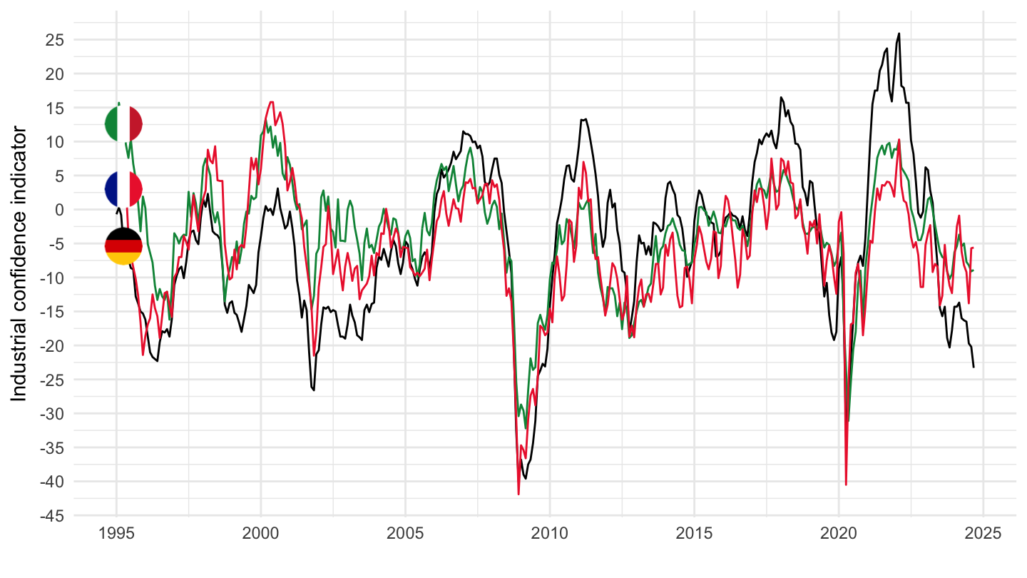
ei_bsin_m_r2 %>%
  filter(indic == "BS-ICI",
         geo %in% c("FR", "DE", "IT"),
         s_adj == "NSA") %>%
  select(geo, time, values) %>%
  group_by(geo) %>%
  left_join(geo, by = "geo") %>%
  mutate(Geo = ifelse(geo == "DE", "Germany", Geo)) %>%
  month_to_date %>%
  filter(date >= as.Date("2000-01-01")) %>%
  left_join(colors, by = c("Geo" = "country")) %>%
  ggplot() + ylab("Industrial confidence indicator") + xlab("") + theme_minimal() +
  geom_line(aes(x = date, y = values, color = color)) +
  scale_color_identity() + add_3flags + theme(legend.position = "none") +
  scale_x_date(breaks = seq(1920, 2025, 5) %>% paste0("-01-01") %>% as.Date,
               labels = date_format("%Y")) +
  scale_y_continuous(breaks = seq(-2000, 2000, 5))
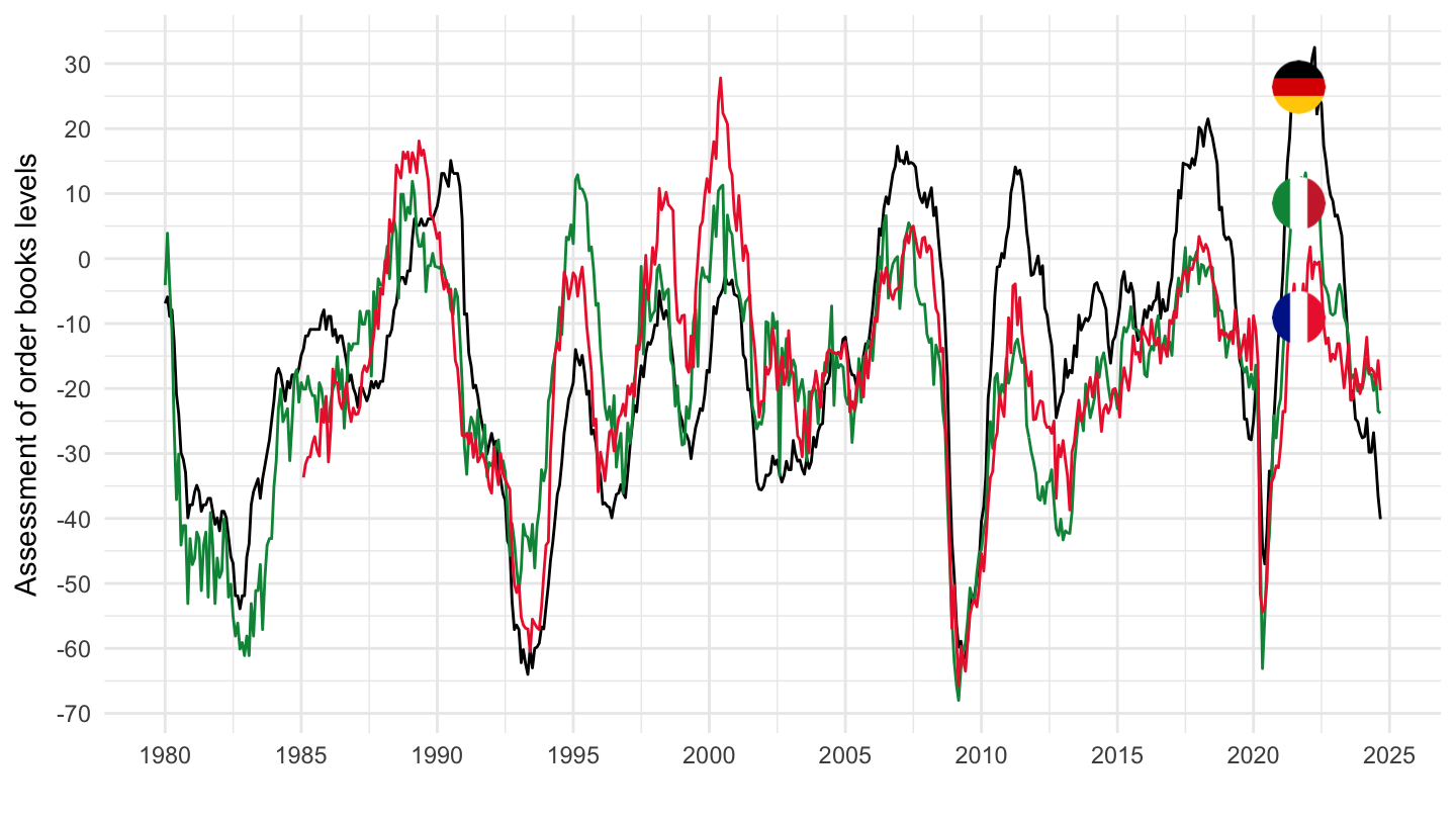
ei_bsin_m_r2 %>%
  filter(indic == "BS-IOB",
         geo %in% c("FR", "DE", "IT"),
         s_adj == "NSA") %>%
  select(geo, time, values) %>%
  left_join(geo, by = "geo") %>%
  mutate(Geo = ifelse(geo == "DE", "Germany", Geo)) %>%
  month_to_date %>%
  left_join(colors, by = c("Geo" = "country")) %>%
  ggplot() + ylab("Assessment of order books levels") + xlab("") + theme_minimal() +
  geom_line(aes(x = date, y = values, color = color)) +
  scale_color_identity() + add_3flags + theme(legend.position = "none") +
  scale_x_date(breaks = seq(1920, 2025, 5) %>% paste0("-01-01") %>% as.Date,
               labels = date_format("%Y")) +
  scale_y_continuous(breaks = seq(-2000, 2000, 10))